Uncertainty measurement for a three heterogeneous information system based on k-nearest neighborhood: Application to unsupervised attribute reduction

Xiaoyan Guo; Yichun Peng; Yu Li

doi:10.1515/jisys-2025-0077

Article Open Access

Uncertainty measurement for a three heterogeneous information system based on k-nearest neighborhood: Application to unsupervised attribute reduction

Xiaoyan Guo , Yichun Peng and Yu Li

Published/Copyright: October 30, 2025

Published by

Become an author with De Gruyter Brill

Submit Manuscript Author Information

From the journal Journal of Intelligent Systems Volume 34 Issue 1

Abstract

The k -nearest-neighbor (KNN) rule is a widely adopted classification technique in machine learning and pattern recognition. Notably, rough set models exhibit a robust capability for decision approximation, making them particularly valuable in handling complex and imprecise data. In practical applications, information systems (IS) often comprise diverse structures of information values. A three-way heterogeneous information system (3HIS) refers to an IS where attribute values encompass three distinct data types: scaled (continuous), ordinal (ranked), and nominal (categorical). This article investigates uncertainty measurement in a 3HIS by leveraging the KNN approach. First, we introduce a specialized distance function designed to compute the dissimilarity between any two information values within each attribute, accounting for the heterogeneity of data types. Building upon this, we propose an enhanced KNN model tailored for a 3HIS, which effectively captures local data structures. By using this model, we construct information granules that facilitate granular computing in heterogeneous data environments. Subsequently, we develop uncertainty quantification tools based on information entropy and information granulation, enabling a rigorous assessment of data inconsistency and ambiguity. To validate the effectiveness of these measurements, we conduct dispersion analysis from a statistical perspective, comparing various uncertainty metrics. Furthermore, we introduce a novel unsupervised attribute reduction algorithm for a 3HIS. The algorithm optimizes feature selection by minimizing redundancy while preserving discriminative power. To evaluate its performance, we employ cluster analysis to demonstrate its efficacy in enhancing data interpret-ability and classification accuracy. These findings provide significant insights into the fundamental nature of uncertainty in a 3HIS.

Keywords: 3HIS; uncertainty measurement; dispersion; k-nearest neighborhood; unsupervised attribute reduction

1 Introduction

1.1 Research background

Uncertainty of datasets, including randomness, fuzziness, vagueness, incompleteness, and inconsistency, is widespread. Uncertainty measurement (UM) can supply new points of view for analyzing data and help us to disclose the substantive characteristics of datasets.

Rough set theory (RST) is a significant tool to deal with uncertainty. This theory only uses internal information, which can be independent of the prior model convention. It can also extract and represent the hidden knowledge in an information system (IS) [1,2]. In rough set theory, knowledge is defined as a family set with indistinguishable relations, so that knowledge has a clear mathematical meaning, then we can use mathematical methods to deal with it. It gives a mathematical method of knowledge discovery.

Information entropy, introduced by Shannon [3], is an important tool for estimating uncertainty. Information granulation is mainly used to study uncertainty of information or knowledge in an IS. All these studies were dedicated to evaluating uncertainty of a set in terms of the partition ability of a knowledge.

Some scholars measured uncertainty of ISs or rough sets by using information entropy and information granulation. For instance, Liang and Qian [4] studied information granules and entropy theory in an IS. Beaubouef et al. [5] came up with a method for measuring the uncertainty of rough sets. Sosa-Cabrera et al. [6] investigated a multivariate approach to the symmetrical UM. Zhao et al. [7] studied complement information entropy for UM in fuzzy rough sets and its applications. Zhang et al. [8] studied UM for interval set information tables based on interval δ -similarity relation. Navarrete et al. [9] considered color smoothing for RGB-D data utilizing entropy information. Huang and Li [10] proposed discernibility measures for fuzzy β -covering. Chen et al. [11] considered UM in an neighborhood IS based on information entropy.

Attribute reduction or feature selection is considered to be one of the important problems in the research of RST [2]. In recent years, attribute reduction has received much attention and some attribute reduction algorithms have been proposed. Wang et al. [12] discussed attribute reduction for hybrid data based on the fuzzy rough iterative computation model. Thuy and Wongthanavasu [13] gave a novel feature selection method for a high-dimensional mixed decision IS. Zhang et al. [14] researched attribute reduction based on the D-S evidence theory in a hybrid IS. Gao et al. [15] considered granular maximum decision entropy-based monotonic uncertainty measure for attribute reduction. Sun et al. [16] proposed feature selection using neighborhood entropy-based uncertainty measures for gene expression data classification. Wang et al. [17] studied feature selection and classification based on directed fuzzy rough sets. An et al. [18] gave robust fuzzy rough approximations with k -nearest-neighbor (KNN) granules for semisupervised feature selection. Xu and Li [19] considered multilabel feature selection for imbalanced data via KNN-based multilabel rough set theory. Dai et al. [20] investigated feature selection based on neighborhood complementary entropy for heterogeneous data. Moreover, Cui et al. [21] introduced adaptive fuzzy neighborhood decision tree, Zhang et al. [22] presented adaptive relative fuzzy rough learning for classification, and Yang et al. [23] proposed adaptive three-way KNN classifier using density-based granular balls.

1.2 Motivation and contributions

Neighborhood rough set is an important model for dealing with real-valued data in the rough set theory. The above series of neighborhood rough sets based on neighborhood information granules have the following disadvantage. For ISs with different distribution densities for different attributes (even when rescaled), the neighborhood parameter that controls the size of information granules should be different for the low-density sample distribution region and the high-density sample distribution region. KNN classification algorithm is a theoretically mature method and one of the important machine learning algorithms. The idea of this method is that in the feature space, if most of the k -nearest (i.e., the closest) samples near a sample belong to a certain category, then the sample also belongs to that category. The model used in KNN algorithm actually corresponds to the partitioning of the feature space. The selection of k , distance measurement, and classification decision rules are the three basic elements of this algorithm. KNN algorithm can not only be used for classification, but also for regression. By identifying the KNN of a sample and assigning the average value of some attribute to a sample, the attribute value of this sample can be obtained.

A 3HIS means an IS whose information values contain three types of data (i.e., scaled type, ordinal type, and nominal type). Considering the powerful functionality of KNN, this article studies UM in a 3HIS based on KNN and neighborhood rough set, applying UM to unsupervised attribute reduction. We summarize the major contributions as follows.

The processing method for different types of data in a 3HIS is provided, and a specific distance function is summarized to calculate the distance between any two information values within each single attribute. Based on KNN and neighborhood rough set, KNN in a 3HIS is proposed.
Information granules in a 3HIS are constructed by using KNN. On this basis, four UMs of a 3HIS are discussed.
Dispersion analysis in statistics to compare four UMs. An unsupervised attribute reduction algorithm for a 3HIS based on KNN is designed, and cluster analysis is performed to evaluate the designed unsupervised attribute reduction.

The writing aim of this study can be outlined as follows.

This study will address the uncertainty measure issue in a 3HIS, using the KNN framework and information entropy tools to assess data fuzziness.
This study will construct an improved KNN model that integrates multiple attribute distances to capture local features of heterogeneous data.
This study will propose the ARHentropy attribute reduction algorithm to balance attribute redundancy and discriminability, providing theoretical support for gene expression data analysis.

1.3 Structure and organization

Figure 1 depicts the flowchart of this article.

Figure 1

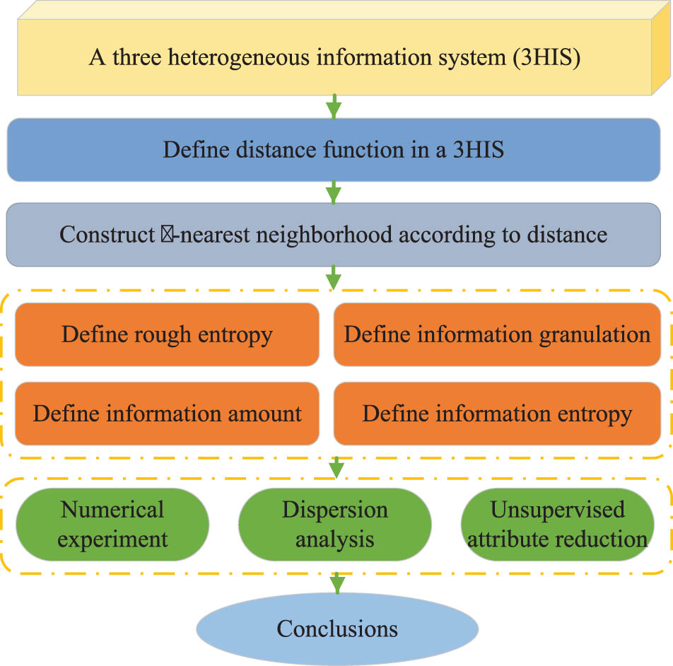
Flowchart of this article. Source: Created by the authors.

The remaining part of this article is organized as follows. Section 2 recalls related concepts about a 3HIS. Section 3 introduces KNN in a 3HIS. Section 4 proposes tools for measuring the uncertainty of a 3HIS based on KNN. Section 5 first conducts numerical experiment to compare four UMs, then executes the dispersion analysis for four UMs, finally presents an unsupervised attribute reduction algorithm, and carries out cluster analysis. Section 6 discusses the advantages and disadvantages of the study. Section 7 summarizes the study.

2 Preliminaries

In this section, we review the notion of fuzzy relations.

Throughout this article, U = { u 1 , u 2 , … , u n } denotes a finite set, 2 U is the family of all subsets of U and ∣ X ∣ represents the cardinality of X ∈ 2 U . Put

△ = { ( u , u ) : u ∈ U } .

Definition 2.1

[1] Let U be a finite set of objects. Suppose that A expresses a finite set of features. Then the ordered pair ( U , A ) is referred to as an IS, if a ∈ A is able to decide a function a : U → V a , where V a = { a ( u ) : u ∈ U } .

Definition 2.2

Let ( U , A ) be an IS. Then ( U , A ) is called a three heterogeneous information system (3HIS), if A contain three types of data (i.e., scaled type, ordinal type and nominal type).

Let ( U , A ) be a 3HIS. Given a ∈ A . If a is scaled or ordinal, then for x ∈ U , normalize

(2.1) a ( x ) ′ = a ( x ) − min { a ( u ) : u ∈ U } max { a ( u ) : u ∈ U } − min { a ( u ) : u ∈ U } .

Definition 2.3

Let ( U , A ) be a 3HIS. Given a ∈ A and u , v ∈ U . Distance between a ( u ) and a ( v ) is defined as follows:

d ( a ( u ) , a ( v ) ) = 0 , if a ( u ) = a ( v ) .

Otherwise,

d ( a ( u ) , a ( v ) ) = ∣ a ( u ) ′ − a ( v ) ′ ∣ , a is scaled 1 − max { a ( u ) ′ − a ( v ) ′ , 0 } , a is ordinal 1 , a is nominal .

Put

d a = ( d ( a ( u i ) , a ( j ) ) ) n × n .

Example 2.4

Table 1 illustrates a 3HIS, where U = { u 1 , u 2 , u 3 , u 4 , u 5 , u 6 , u 7 , u 8 } and A = { a 1 , a 2 , a 3 , a 4 , a 5 , a 6 } .

Table 1

A 3HIS ( U , A )

U	a 1	a 2	a 3	a 4	a 5	a 6
u 1	5.08	2.67	Good	Small	Red	China
u 2	9.92	3.31	Average	Middle	Green	USA
u 3	7.67	4.59	Good	Big	Blue	USA
u 4	15.18	4.41	Average	Middle	Blue	China
u 5	7.81	2.09	Pass	Big	Green	UK
u 6	18.23	6.31	Average	Big	Blue	China
u 7	17.05	2.76	Average	Middle	Blue	USA
u 8	9.63	3.17	Excellent	Small	Red	UK

First, features a 3 , a 4 , a 5 , and a 6 can be digitized as follows. Obviously, the feature values of a 3 and a 4 are arranged in a consecutive order, namely, features a 3 and a 4 are ordinal. Thus, the p a s s , a v e r a g e , g o o d , and e x c e l l e n t of feature a 3 can be assigned to 1, 2, 3, and 4, respectively. Similarly, the s m a l l , m i d d l e , and b i g of feature a 4 are respectively designated to 1, 2, and 3. For a 5 and a 6 , their feature values are not particular order, namely, features a 5 and a 6 are nominal. Consequently, the r e d , g r e e n , and b l u e are, respectively given to 1, 2, and 3 for feature a 5 , while the C h i n a , U S A , and U K are respectively allocated to 1, 2, and 3 for feature a 6 . Features a 1 , a 2 , a 3 , and a 4 are first normalized with regards to Formula (2.1), then Formula (2.3) is utilized to calculate the distance of two objects to obtain the distances of pairwise objects.

We can obtain that

d a 1 = 0 0.37 0.20 0.77 0.21 1.00 0.91 0.35 0.37 0 0.17 0.40 0.16 0.63 0.54 0.02 0.20 0.17 0 0.57 0.01 0.80 0.71 0.15 0.77 0.40 0.57 0 0.56 0.23 0.14 0.42 0.21 0.16 0.01 0.56 0 0.79 0.70 0.14 1.00 0.63 0.80 0.23 0.79 0 0.09 0.65 0.91 0.54 0.71 0.14 0.70 0.09 0 0.56 0.35 0.02 0.15 0.42 0.14 0.65 0.56 0 ,

d a 2 = 0 0.15 0.46 0.41 0.14 0.86 0.02 0.12 0.15 0 0.30 0.26 0.29 0.71 0.13 0.03 0.46 0.30 0 0.04 0.60 0.41 0.43 0.34 0.41 0.26 0.04 0 0.55 0.45 0.39 0.29 0.14 0.29 0.59 0.55 0 1.00 0.16 0.26 0.86 0.71 0.41 0.45 1.00 0 0.84 0.74 0.02 0.13 0.43 0.39 0.16 0.84 0 0.10 0.12 0.03 0.34 0.29 0.26 0.74 0.10 0 ,

d a 3 = 0 0.67 0 0.67 0.33 0.67 0.67 1 0.67 0 1 0 0.67 0 0 1 0 1 0 0.67 0.33 0.67 0.67 1 0.67 0 0.67 0 0.67 0 0 1 0.33 0.67 0.33 0.67 0 1 1 1 0.67 0 0.67 0 1 0 0 1 0.67 0 0.67 0 1 0 0 1 1 1 1 1 1 1 1 0 ,

d a 4 = 0 1 1 1 1 1 1 0 1 0 1 0 1 1 0 0.5 1 1 0 0.5 0 0 0.5 0 1 0 0.5 0 1 1 0 0.5 1 1 0 1 0 0 0.5 0 1 1 0 1 0 0 0.5 0 1 0 0.5 0 0.5 0.5 0 0.5 0 0.5 0 0.5 0 0 0.5 0 ,

d a 5 = 0 1 1 1 1 1 1 0 1 0 1 1 0 1 1 1 1 1 0 0 1 0 0 1 1 1 0 0 1 0 0 1 1 0 1 1 0 1 1 1 1 1 0 0 1 0 0 1 1 1 0 0 1 0 0 1 0 1 1 1 1 1 1 0 ,

d a 6 = 0 1 1 0 1 0 1 1 1 0 0 1 1 1 0 1 1 0 0 1 1 1 0 1 0 1 1 0 1 0 1 1 1 1 1 1 0 1 1 0 0 1 1 0 1 0 1 1 1 0 0 1 1 1 0 1 1 1 1 1 0 1 1 0 .

Definition 2.5

Let ( U , A ) be a 3HIS with B ⊆ A . Given λ ∈ [ 0 , 1 ] . Define

N B λ = { ( u , v ) ∈ U × U : ∀ a ∈ B , d ( a ( u ) , a ( v ) ) ≤ λ } , N B λ ( u ) = { v ∈ U : ( u , v ) ∈ N B λ } .

Then N B λ and N B λ ( u ) are called λ -neighborhood relation on U respect with to B and λ -neighborhood of u respect with to B , respectively.

Example 2.6

(Continued from Example 2.4)

Let u = u 1 , B = { a 1 , a 2 } and λ = 0.6 . The N B λ ( u 1 ) is calculated as follows. The set s e t 1 = { u 1 , u 2 , u 3 , u 5 , u 8 } is the λ -neighborhood of u 1 with respect to { a 1 } , while the set s e t 2 = { u 1 , u 2 , u 3 , u 4 , u 5 , u 7 , u 8 } is the λ -neighborhood of u 1 with respect to { a 2 } . The intersection of s e t 1 and s e t 2 is the λ -neighborhood of u 1 in regards to B = { a 1 , a 2 } . Namely, N B λ ( u 1 ) = { u 1 , u 2 , u 3 , u 5 , u 8 } . Table 2 lists the N B λ ( u i ) of U = { u i : i ∈ { 1 , … , 8 } } respect with to B = { a 1 , a 2 } .

Table 2

λ -neighborhood of U respect with to B = { a 1 , a 2 }

U = { u i }	N B λ ( u i )
u 1	{ u 1 , u 2 , u 3 , u 5 , u 8 }
u 2	{ u 1 , u 2 , u 3 , u 4 , u 5 , u 7 , u 8 }
u 3	{ u 1 , u 2 , u 3 , u 4 , u 5 , u 8 }
u 4	{ u 2 , u 3 , u 4 , u 5 , u 6 , u 7 , u 8 }
u 5	{ u 1 , u 2 , u 3 , u 4 , u 5 , u 8 }
u 6	{ u 4 , u 6 }
u 7	{ u 2 , u 4 , u 7 , u 8 }
u 8	{ u 1 , u 2 , u 3 , u 4 , u 5 , u 7 , u 8 }

N B λ is reflexive and symmetric. N B λ ( u ) can be viewed as an neighborhood information granule, which is called λ -neighborhood information granule.

Below, we use λ -neighborhood information granule to construct KNN.

3 KNN in a 3HIS

Definition 3.1

Let ( U , A ) be a 3HIS with a ∈ A and u ∈ U . Given k ∈ N . Denote u 0 = u . ∀ i ∈ { 1 , 2 , … , k − 1 } , put

u i = arg min { d ( a ( u ) , a ( v ) ) : v ∈ U − { u 0 , u 1 , … , u i − 1 } }

d ( a ( u ) , a ( u i ) ) = min { d ( a ( u ) , a ( v ) ) } ,

where v ∈ U − { { u 0 , u 1 , … , u i − 1 } }

Define

a k ( u ) = { u 0 , u 1 , … , u k − 1 } .

Obviously, ∀ i ∈ { 1 , 2 , … , k − 1 } ,

d ( a ( u ) , a ( u i − 1 ) ) ≤ d ( a ( u ) , a ( u i ) ) .

Definition 3.2

Let ( U , A ) be a 3HIS with B ⊆ A and u ∈ U . Given k ∈ N . Define

B k ( u ) = ⋂ a ∈ B a k ( u ) , B N k , λ ( u ) = B k ( u ) ∩ N B λ ( u ) .

Then B k ( u ) is called k -nearest of u with respect to B , and B N k , λ ( u ) is called KNN of u with respect to B .

Example 3.3

(Continued from Example 2.4)

Let u = u 1 , B = { a 1 , a 2 } , λ = 0.6 , and k = 5 . According to Definition 3.1, a 1 k ( u 1 ) = { u 1 , u 3 , u 5 , u 8 , u 2 } , a 2 k ( u 1 ) = { u 1 , u 7 , u 8 , u 5 , u 2 } . In terms of Definition 3.2, B k ( u 1 ) = a 1 k ( u 1 ) ∩ a 2 k ( u 1 ) = { u 1 , u 5 , u 8 , u 2 } . From Table 2, we can find that u 1 = { u 1 , u 2 , u 3 , u 5 , u 8 } . Thus, B N k , λ ( u 1 ) = B k ( u 1 ) ∩ N B λ ( u 1 ) = { u 1 , u 2 , u 5 , u 8 } . Table 3 illustrates the B N k , λ ( u i ) of U = { u i : i ∈ { 1 , … , 8 } } respect with to B = { a 1 , a 2 } .

Table 3

KNN of U respect with to B = { a 1 , a 2 }

U = { u i }	B N k , λ ( u i )
u 1	{ u 1 , u 2 , u 5 , u 8 }
u 2	{ u 1 , u 2 , u 8 }
u 3	{ u 2 , u 3 , u 8 }
u 4	{ u 2 , u 4 , u 7 , u 8 }
u 5	{ u 1 , u 2 , u 5 , u 8 }
u 6	{ u 4 , u 6 }
u 7	{ u 2 , u 7 , u 8 }
u 8	{ u 1 , u 2 , u 5 , u 8 }

Proposition 3.4

Let ( U , A ) be a 3HIS. Given u ∈ U .

If B ⊆ C ⊆ A , then ∀ k , C N k , λ ( u ) ⊆ B N k , λ ( u ) .
If k 1 ≤ k 2 , then ∀ B ⊆ A , B N k 1 , λ ( u ) ⊆ B N k 2 , λ ( u ) .
If 0 ≤ λ 1 ≤ λ 2 ≤ 1 , then ∀ B ⊆ A , B N k , λ 1 ( u ) ⊆ B N k , λ 2 ( u ) .

Proof

(1) Suppose B ⊆ C ⊆ A . Obviously,

C k ( u ) ⊆ B k ( u ) , N C λ ( u ) ⊆ N B λ ( u ) .

Thus, C N k , λ ( u ) ⊆ B N k , λ ( u ) .

(2) Suppose k 1 ≤ k 2 . Then B k 1 ( u ) ⊆ B k 2 ( u ) .

B k 1 ( u ) ∩ N B λ ( u ) ⊆ B k 2 ( u ) ∩ N B λ ( u ) .

Thus, B N k 1 , λ ( u ) ⊆ B N k 2 , λ ( u ) .

( 3 ) Suppose 0 ≤ λ 1 ≤ λ 2 ≤ 1 . Then N B λ 1 ( u ) ⊆ N B λ 2 ( u ) .

B k ( u ) ∩ N B λ 1 ( u ) ⊆ B k ( u ) ∩ N B λ 2 ( u ) .

Thus, B N k , λ 1 ( u ) ⊆ B N k , λ 2 ( u ) . □

Put

B N k , λ = { ( u , v ) ∈ U × U : v ∈ B N k , λ ( u ) } ;

Then B N k , λ is reflexive. However, it does not satisfy symmetry and transitivity.

4 Measuring the uncertainty of a 3HIS

In this section, we propose some tools for measuring the uncertainty of a 3HIS.

4.1 Granularity measures for a 3HIS

Definition 4.1

Suppose that ( U , A ) is a 3HIS. Given B ⊆ A , k ∈ N and λ ∈ [ 0 , 1 ] . Then information granulation of the subsystem ( U , B ) is defined as follows:

(4.1) G N k , λ ( B ) = ∑ i = 1 n 1 n 2 ∣ B N k , λ ( u i ) ∣ .

Proposition 4.2

Suppose that ( U , A ) is a 3HIS. Given B ⊆ A , k ∈ N and λ ∈ [ 0 , 1 ] . Then

(4.2) 1 n ≤ G N k , λ ( B ) ≤ k n .

If B N k , λ = △ , then G N k , λ reaches the minimum value 1 n .

Proof

∀ i , 1 ≤ ∣ B N k , λ ( u i ) ∣ ≤ k . Then

n ≤ ∑ i = 1 n ∣ B N k , λ ( u i ) ∣ ≤ n k .

Thus,

1 n ≤ G N k , λ ( B ) ≤ k n .

If B N k , λ = △ , then ∀ i , B N k , λ ( u i ) = { u i } , and so G N k , λ ( B ) = 1 n .□

Proposition 4.3

Let ( U , A ) be a 3HIS.

If B ⊆ C ⊆ A , then ∀ k , ∀ λ , G N k , λ ( C ) ≤ G N k , λ ( B ) .
If k 1 ≤ k 2 , then ∀ B , ∀ λ , G N k 1 , λ ( B ) ≤ G N k 2 , λ ( B ) .
If 0 ≤ λ 1 ≤ λ 2 ≤ 1 , then ∀ B , ∀ k , G N k , λ 1 ( B ) ≤ G N k , λ 2 ( B ) .

Proof

It can be proved by Proposition 3.4.□

4.2 Entropy measure for a 3HIS

Definition 4.4

Suppose that ( U , A ) is a 3HIS. Given B ⊆ A , k ∈ N and λ ∈ [ 0 , 1 ] . Then rough entropy of the subsystem ( U , B ) is defined as follows:

(4.3) ( E r ) N k , λ ( B ) = − ∑ i = 1 n 1 n log 2 1 ∣ B N k , λ ( u i ) ∣ .

Proposition 4.5

Let ( U , A ) be a 3HIS. Given B ⊆ A , k ∈ N , and λ ∈ [ 0 , 1 ] . Then

(4.4) 0 ≤ ( E r ) N k , λ ( B ) ≤ log 2 k .

If B N k , λ = △ , then ( E r ) N k , λ reaches the minimum value 0.

Proof

( 1 ) ∀ i , 1 ≤ ∣ B N k , λ ( u i ) ∣ ≤ k . Then

Then ∀ i

0 ≤ − log 2 1 ∣ B N k , λ ( u i ) ∣ = log 2 ∣ B N k , λ ( u i ) ∣ ≤ log 2 k .

Thus,

0 ≤ ( E r ) N k , λ ( B ) ≤ log 2 k .

( 2 ) Suppose B N k , λ = △ . Then ∀ i , B N k , λ ( u i ) = { u i } and so ( E r ) N k , λ ( B ) = 0 . □

Proposition 4.6

Let ( U , A ) be a 3HIS.

If B ⊆ C ⊆ A , then ∀ k , ∀ λ , ( E r ) N k , λ ( C ) ≤ ( E r ) N k , λ ( B ) .
If k 1 ≤ k 2 , then ∀ B , ∀ λ , ( E r ) N k 1 , λ ( B ) ≤ ( E r ) N k 2 , λ ( B ) .
If 0 ≤ λ 1 ≤ λ 2 ≤ 1 , then ∀ B , ∀ k , ( E r ) N k , λ 1 ( B ) ≤ ( E r ) N k , λ 2 ( B ) .

Proof

(1) Since B ⊆ C ⊆ A , by Proposition 3.4, we have

∀ i , C N k , λ ( u i ) ⊆ B N k , λ ( u i ) .

Then ∀ i , log 2 ∣ C N k , λ ( u i ) ∣ ≤ log 2 ∣ B N k , λ ( u i ) ∣ .

By Definition 4.4,

( E r ) N k , λ ( B ) = 1 n ∑ i = 1 n log 2 ∣ B N k , λ ( u i ) ∣ , ( E r ) N k , λ ( C ) = 1 n ∑ i = 1 n log 2 ∣ C N k , λ ( u i ) ∣ .

Hence,

( E r ) N k , λ ( C ) ≤ ( E r ) N k , λ ( B ) .

(2) Since k 1 ≤ k 2 , by Proposition 3.4, we have

∀ i , B N k 1 , λ ( u i ) ⊆ B N k 2 , λ ( u i ) .

Then ∀ i , log 2 ∣ B N k 1 , λ ( u i ) ∣ ≤ log 2 ∣ B N k 2 , λ ( u i ) ∣ .

By Definition 4.4,

( E r ) N k 1 , λ ( B ) = 1 n ∑ i = 1 n log 2 ∣ B N k 1 , λ ( u i ) ∣ , ( E r ) N k 2 , λ ( B ) = 1 n ∑ i = 1 n log 2 ∣ B N k 2 , λ ( u i ) ∣ .

Hence,

( E r ) N k 1 , λ ( B ) ≤ ( E r ) N k 2 , λ ( B ) .

(3) Since 0 ≤ λ 1 ≤ λ 2 ≤ 1 , by Proposition 3.4, we have

∀ i , B N k , λ 1 ( u i ) ⊆ B N k , λ 2 ( u i ) .

Then ∀ i , log 2 ∣ B N k , λ 1 ( u i ) ∣ ≤ log 2 ∣ B N k , λ 2 ( u i ) ∣ .

By Definition 4.4,

( E r ) N k , λ 1 ( B ) = 1 n ∑ i = 1 n log 2 ∣ B N k , λ 1 ( u i ) ∣ , ( E r ) N k , λ 2 ( B ) = 1 n ∑ i = 1 n log 2 ∣ B N k , λ 2 ( u i ) ∣ .

Hence,

□ ( E r ) N k , λ 1 ( B ) ≤ ( E r ) N k , λ 2 ( B ) .

Definition 4.7

Let ( U , A ) be a 3HIS. Given B ⊆ A , k ∈ N and λ ∈ [ 0 , 1 ] . Then information entropy of the subsystem ( U , B ) is defined as follows:

(4.5) H N k , λ ( B ) = − ∑ i = 1 n 1 n log 2 ∣ B N k , λ ( u i ) ∣ n .

Theorem 4.8

Let ( U , A ) be a 3HIS. Given B ⊆ A , k ∈ N , and λ ∈ [ 0 , 1 ] . Then

(4.6) ( E r ) N k , λ ( B ) + H N k , λ ( B ) = log 2 n .

Proof

By Definitions 4.4 and 4.7,

( E r ) N k , λ ( B ) = − ∑ i = 1 n 1 n log 2 1 ∣ B N k , λ ( u i ) ∣ , H N k , λ ( B ) = − ∑ i = 1 n 1 n log 2 ∣ B N k , λ ( u i ) ∣ n .

Then

(4.7)□ ( E r ) N k , λ ( B ) + H N k , λ ( B ) = − ∑ i = 1 n 1 n log 2 1 ∣ B N k , λ ( u i ) ∣ − ∑ i = 1 n 1 n log 2 ∣ B N k , λ ( u i ) ∣ n = − 1 n ∑ i = 1 n log 2 1 ∣ B N k , λ ( u i ) ∣ + log 2 ∣ B N k , λ ( u i ) ∣ n = − 1 n ∑ j = 1 n log 2 1 n = log 2 n .

Corollary 4.9

Let ( U , A ) be a 3HIS. Given B ⊆ A , k ∈ N , and λ ∈ [ 0 , 1 ] . Then

(4.8) log 2 n k ≤ H N k , λ ( B ) ≤ log 2 n .

If B N k , λ = △ , then H N k , λ reaches the maximum value log 2 n .

Proof

It can be obtained by Proposition 4.5 and Theorem 4.8.□

Corollary 4.10

Let ( U , A ) be a 3HIS.

If B ⊆ C ⊆ A , then ∀ k , ∀ λ , H N k , λ ( B ) ≤ H N k , λ ( C ) .
If k 1 ≤ k 2 , then ∀ B , ∀ λ , H N k 2 , λ ( B ) ≤ H N k 1 , λ ( B ) .
If 0 ≤ λ 1 ≤ λ 2 ≤ 1 , then ∀ B , ∀ k , H N k , λ 2 ( B ) ≤ H N k , λ 1 ( B ) .

Proof

It can be obtained by Proposition 4.6 and Theorem 4.8.□

This corollary shows that the information entropy increases when the information structure becomes finer, and it decreases when information structure becomes coarser.

4.3 Information amount in a 3HIS

Definition 4.11

Let ( U , A ) be a 3HIS. Given B ⊆ A , k ∈ N and λ ∈ [ 0 , 1 ] . Then information amount of the subsystem ( U , B ) is defined as follows:

(4.9) E N k , λ ( B ) = ∑ i = 1 n 1 n 1 − ∣ B N k , λ ( u i ) ∣ n .

Example 4.12

(Continued from Examples 2.4 and 3.3)

Let λ = 0.6 and k = 5 . Denote B i = { a 1 , … , a i } ( i = 1 , … , 6 ) . Definitions 4.1, 4.4, 4.7, and 4.11 are, respectively, utilized to calculate information granulation G N k , λ ( B ) , rough entropy ( E r ) N k , λ ( B ) , information entropy H N k , λ ( B ) , and information amount E N k , λ ( B ) of ( U , B ) . Four UMs are exemplified in Table 4.

Table 4

Uncertainty measures of ( U , B i )

B i	G N k , λ ( B i )	( E r ) N k , λ ( B i )	H N k , λ ( B i )	E N k , λ ( B i )
B 1	0.5938	2.2298	0.7702	0.4063
B 2	0.4219	1.7194	1.2806	0.5781
B 3	0.2188	0.6981	2.3019	0.7813
B 4	0.1719	0.3231	2.6769	0.8281
B 5	0.1406	0.1250	2.8750	0.8594
B 6	0.1250	0.0000	3.0000	0.8750

Theorem 4.13

Let ( U , A ) be a 3HIS. Given B ⊆ A , k ∈ N , and λ ∈ [ 0 , 1 ] . Then

(4.10) G N k , λ ( B ) + E N k , λ ( B ) = 1 .

Proof

By Definition 4.1,

G N k , λ ( B ) = ∑ i = 1 n 1 n 2 ∣ B N k , λ ( u i ) ∣ .

By Definition 4.11,

E N k , λ ( B ) = ∑ i = 1 n 1 n 1 − ∣ B N k , λ ( u i ) ∣ n .

Then

G N k , λ ( B ) + E N k , λ ( B ) = 1 n 2 ∑ i = 1 n ∣ B N k , λ ( u i ) ∣ + ∑ i = 1 n 1 n 1 − ∣ B N k , λ ( u i ) ∣ n = 1 n ∑ i = 1 n ∣ B N k , λ ( u i ) ∣ n + 1 − ∣ B N k , λ ( u i ) ∣ n = 1 n ∑ j = 1 n 1 = 1 .

□ G N k , λ ( B ) + E N k , λ ( B ) = 1 .

Corollary 4.14

Let ( U , A ) be a 3HIS. Given B ⊆ A , k ∈ N and λ ∈ [ 0 , 1 ] . Then

(4.11) 1 − k n ≤ E N k , λ ( B ) ≤ 1 − 1 n .

If B N k , λ = △ , then E N k , λ reaches the maximum value 1 − 1 n .

Proof

It can be proved by Proposition 4.2 and Theorem 4.13.□

Corollary 4.15

Let ( U , A ) be a 3HIS.

If B ⊆ C ⊆ A , then ∀ k , ∀ λ , E N k , λ ( B ) ≤ E N k , λ ( C ) .
If k 1 ≤ k 2 , then ∀ B , ∀ λ , E N k 2 , λ ( B ) ≤ E N k 1 , λ ( B ) .
If 0 ≤ λ 1 ≤ λ 2 ≤ 1 , then ∀ B , ∀ k , E N k , λ 2 ( B ) ≤ E N k , λ 1 ( B ) .

Proof

It can be obtained by Proposition 4.3 and Theorem 4.13.□

5 Numerical experiments and unsupervised attribute reduction

This section offers several UCI datasets as a 3HIS for evaluating the suggested unsupervised attribute reduction algorithm. It first compares four UMs for each 3HIS, then implements the dispersion analyses, next presents an unsupervised attribute reduction algorithm ( A R H e n t r o p y ), an finally carries out cluster analyses to evaluate the performances by introducing Silhouette coefficient (SC) and Davies-Bouldin index (DBI).

5.1 Numerical experiments

Six datasets from the UCI (Repository of machine learning databases) are selected for a numerical experiment, as shown in Table 5. The details of these datasets are outlined in the table. In addition, four UMs of a 3HIS are compared.

Table 5

Datasets from UCI

Datasets	#Objects	#Features	#Scaled	#Ordinal	#Nominal
Hepatitis [24]	155	20	2	4	14
Automobile [25]	205	26	15	1	10
ILPD [26]	583	11	5	4	2
AIDS [27]	2,139	24	8	3	13
PredictStudents [28]	4,424	37	17	2	18
SUPPORT2 [29]	9,105	45	29	5	11

The parameters of four UMs are setup as follows:

k = # Objects 10 , λ = 0.6 .

The hepatitis dataset may express a 3HIS ( U 1 , A 1 ) with ∣ U 1 ∣ = 155 , ∣ A 1 ∣ = 20 . Denote B i = { a 1 , … , a i } ( i = 1 , … , 20 ) . Four UMs on hepatitis are defined as follows:

G N k , λ ( H e p a t i t i s ) = { G N k , λ ( B 1 ) , … , G N k , λ ( B 20 ) } ( E r ) N k , λ ( H e p a t i t i s ) = { ( E r ) N k , λ ( B 1 ) , … , ( E r ) N k , λ ( B 20 } ) H N k , λ ( H e p a t i t i s ) = { H N k , λ ( B 1 ) , … , H N k , λ ( B 20 ) } E N k , λ ( H e p a t i t i s ) = { E N k , λ ( B 1 ) , … , E N k , λ ( B 20 ) } .

The automobile dataset may express a 3HIS ( U 2 , A 2 ) with ∣ U 2 ∣ = 205 , ∣ A 2 ∣ = 26 . Denote B i = { a 1 , … , a i } ( i = 1 , … , 26 ) . Four UMs on automobile are formulated as follows:

G N k , λ ( A u t o m o b i l e ) = { G N k , λ ( B 1 ) , … , G N k , λ ( B 26 ) } ( E r ) N k , λ ( A u t o m o b i l e ) = { ( E r ) N k , λ ( B 1 ) , … , ( E r ) N k , λ ( B 26 } ) H N k , λ ( A u t o m o b i l e ) = { H N k , λ ( B 1 ) , … , H N k , λ ( B 26 ) } E N k , λ ( A u t o m o b i l e ) = { E N k , λ ( B 1 ) , … , E N k , λ ( B 26 ) } .

The ILPD dataset may express a 3HIS ( U 3 , A 3 ) with ∣ U 3 ∣ = 583 , ∣ A 3 ∣ = 11 . Denote B i = { a 1 , … , a i } ( i = 1 , … , 11 ) . Four UMs on ILPD are derived as follows:

G N k , λ ( I L P D ) = { G N k , λ ( B 1 ) , … , G N k , λ ( B 11 ) } ( E r ) N k , λ ( I L P D ) = { ( E r ) N k , λ ( B 1 ) , … , ( E r ) N k , λ ( B 11 } ) H N k , λ ( I L P D ) = { H N k , λ ( B 1 ) , … , H N k , λ ( B 11 ) } E N k , λ ( I L P D ) = { E N k , λ ( B 1 ) , … , E N k , λ ( B 11 ) } .

The AIDS dataset may express a 3HIS ( U 4 , A 4 ) with ∣ U 4 ∣ = 2,139 , ∣ A 4 ∣ = 24 . Denote B i = { a 1 , … , a i } ( i = 1 , … , 24 ) . Four measures of uncertainty on AIDS are outlined as follows:

G N k , λ ( A I D S ) = { G N k , λ ( B 1 ) , … , G N k , λ ( B 24 ) } ( E r ) N k , λ ( A I D S ) = { ( E r ) N k , λ ( B 1 ) , … , ( E r ) N k , λ ( B 24 } ) H N k , λ ( A I D S ) = { H N k , λ ( B 1 ) , … , H N k , λ ( B 24 ) } E N k , λ ( A I D S ) = { E N k , λ ( B 1 ) , … , E N k , λ ( B 24 ) } .

The PredictStudents dataset may express a 3HIS ( U 5 , A 5 ) with ∣ U 5 ∣ = 4,424 , ∣ A 5 ∣ = 37 . Denote B i = { a 1 , … , a i } ( i = 1 , … , 37 ) . Four measures of uncertainty on PredictStudents are identified as follows:

G N k , λ ( P r e d i c t S t u d e n t s ) = { G N k , λ ( B 1 ) , … , G N k , λ ( B 37 ) } ( E r ) N k , λ ( P r e d i c t S t u d e n t s ) = { ( E r ) N k , λ ( B 1 ) , … , ( E r ) N k , λ ( B 37 } ) H N k , λ ( P r e d i c t S t u d e n t s ) = { H N k , λ ( B 1 ) , … , H N k , λ ( B 37 ) } E N k , λ ( P r e d i c t S t u d e n t s ) = { E N k , λ ( B 1 ) , … , E N k , λ ( B 37 ) } .

The SUPPORT2 dataset may express a 3HIS ( U 6 , A 6 ) with ∣ U 6 ∣ = 9,105 , ∣ A 6 ∣ = 45 . Denote B i = { a 1 , … , a i } ( i = 1 , … , 45 ) . Four measures of uncertainty on diabetes are determined as follows:

G N k , λ ( S U P P O R T 2 ) = { G N k , λ ( B 1 ) , … , G N k , λ ( B 45 ) } ( E r ) N k , λ ( S U P P O R T 2 ) = { ( E r ) N k , λ ( B 1 ) , … , ( E r ) N k , λ ( B 45 } ) H N k , λ ( S U P P O R T 2 ) = { H N k , λ ( B 1 ) , … , H N k , λ ( B 45 ) } E N k , λ ( S U P P O R T 2 ) = { E N k , λ ( B 1 ) , … , E N k , λ ( B 45 ) } .

Figure 2 illustrates that four measures of uncertainty on six datasets have a similar situation. Namely, the information granulation curves with black and rough entropy curves with red decline with the increase of the cardinality of B i , whereas the information entropy curves with blue and information amount curves with brown upgrade with the increase of the cardinality of B i . This means that both information granulation G N k , λ ( B i ) and rough entropy ( E r ) N k , λ ( B i ) are monotonically decreasing when the number of features in subsystem increases, while both information entropy H N k , λ ( B i ) , and information amount E N k , λ ( B i ) are monotonically increasing when the number of features in subsystem increases. Thus, the information granulation G N k , λ ( B i ) , rough entropy ( E r ) N k , λ ( B i ) , information entropy H N k , λ ( B i ) , and information amount E N k , λ ( B i ) can be employed to evaluate the uncertainty of a 3HIS.

Figure 2

Four measures of uncertainty for six 3HISs. Source: Created by the authors.

In addition, Figure 2 also depicts that the alterations in information granulation G N k , λ ( B i ) and information amount E N k , λ ( B i ) curves are relatively insignificant. For six datasets, the G N k , λ ( B i ) approximates 0 whereas the E N k , λ ( B i ) is close to 1. Nevertheless, the alterations in information entropy H N k , λ ( B i ) and rough entropy ( E r ) N k , λ ( B i ) curves are quite significant, particularly in the early stages. Consequently, the information entropy H N k , λ ( B i ) and rough entropy ( E r ) N k , λ ( B i ) offer a marked advantage in comparison to the information granulation G N k , λ ( B i ) and information amount E N k , λ ( B i ) in terms of measuring uncertainty.

5.2 Dispersion analyses

Statistical research often involves studying the dispersion degree of a dataset. The dispersion degree can be measured by difference measures, such as range, point difference, average difference, standard deviation, and dispersion coefficient. This study utilizes the dispersion coefficient to evaluate the dispersion degree of four UMs. The dispersion coefficient is mainly utilized to compare the amount of dispersion between multiple group of data. A high dispersion coefficient indicates a large quantity of data dispersion, while a low dispersion coefficient implies a small degree of data dispersion.

For a given dataset X = { x 1 , … , x n } , the mean value, standard deviation, and dispersion coefficient of X can be represented by x ¯ , σ ( X ) and V S ( X ) , respectively. They are, respectively, formulated as follows.

x ¯ = 1 n ∑ i = 1 n x i , σ ( X ) = 1 n ∑ i = 1 n ( x i − x ¯ ) 2 , V S ( X ) = σ ( X ) x ¯ .

According to four measures of uncertainty on six datasets, their dispersion coefficient are calculated in terms of the aforementioned formulas. Figure 3 depicts that the V S -values of four UMs on six datasets.

Figure 3

V S -values of four UMs on six datasets. Source: Created by the authors.

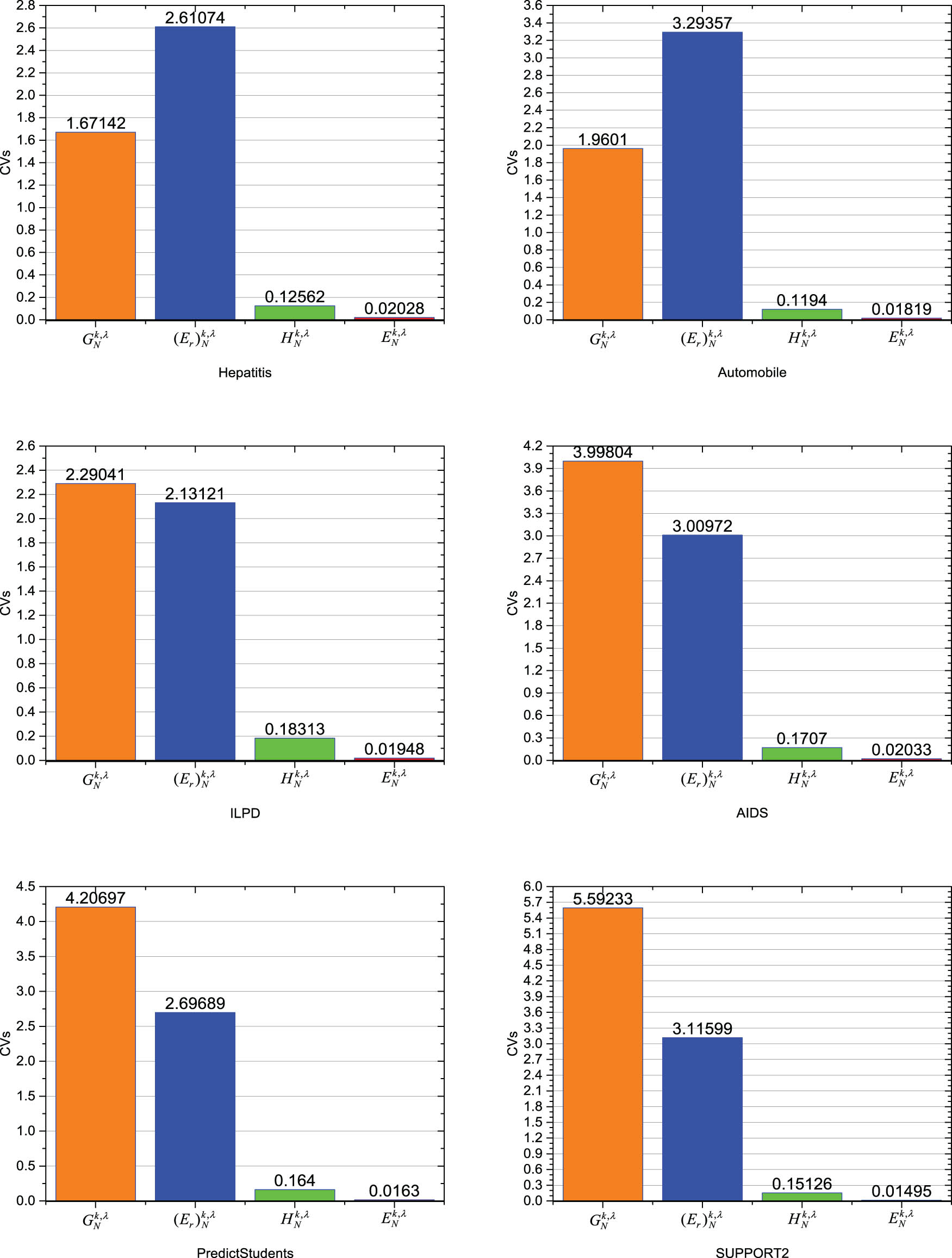
By examining Figure 3, it is evident that the information amount E N k , λ has the lowest values in six datasets, while the information entropy H N k , λ is the second lowest, and the information granulation G N k , λ ( B i ) and rough entropy ( E r ) N k , λ ( B i ) occupy the third or fourth position. This denotes that the information amount E N k , λ and information entropy H N k , λ take advantage over the information granulation G N k , λ ( B i ) and rough entropy ( E r ) N k , λ ( B i ) in measuring uncertainty of a 3HIS.

5.3 Unsupervised attribute reduction

This subsection first presents an unsupervised attribute reduction algorithm ( A R H e n t r o p y ), then offers several UCI datasets as a 3HIS for evaluating the A R H e n t r o p y , finally carries out cluster analyses on several 3HISs, and the resulting reducts after applying A R H e n t r o p y , to compare their performances.

5.3.1 Unsupervised attribute reduction algorithm in a 3HIS

This subsection introduces an unsupervised attribute reduction algorithm utilizing information entropy and evaluates its cost-effectiveness by examining its time complexity and space complexities.

Algorithm 1: Unsupervised attribute reduction in a 3HIS utilizing information entropy ( ARHentropy )
Input: A 3 H I S ( U , A )
Output: A reduct B
B ← random permutation of A
B 1 ← B
for each a ∈ B 1 do
B b e f o r e ← B B ← B − { a } if H N k , λ ( B ) ≠ H N k , λ ( B b e f o r e ) then ∣ B ← B b e f o r e end
end
return B

Algorithm 1 is designed as a heuristic search strategy to obtain one reduct of a 3HIS. It commences with permutation of the sets A containing all attributes and then eliminates the superfluous attribute when the subset B after removing the attribute is a coordination subset of A . If the information entropy of the subset B is equal to that of A , then the attribute can be removed, otherwise it cannot be eliminated and B is restored to the subset before removing the attribute. Hence, each loop will remove 1 or 0 attribute until all attributes are checked. As Algorithm 1 commences with permutation of the sets A , its each implementation may obtain different reduct.

To evaluate the cost-effectiveness of an algorithm, its time and space complexities can be taken into account. The big O notation is a commonly used method for quantifying the running time and required storage space of an algorithm, namely, time and space complexities.

Let ∣ U ∣ = n , ∣ A ∣ = m . The time complexity of Algorithm 1 is determined by the “for” loop, which obviously runs for m iterations. As per Definition 4.7, the time complexities for computing H N k , λ ( B ) and H N k , λ ( B b e f o r e ) are both O ( n ) . Consequently, the time complexity of Algorithm 1 is O ( n m ) . Algorithm 1 requires n × m storage space for input variable ( U , A ) , hence, its space complexity is also O ( n m ) .

5.3.2 Datasets

The subsection selects six datasets of varying complexities from the UCI, namely, L y m p h o g r a p h y , H e p a t i t i s , A u t o m o b i l e , I L P D , C r e d i t , and A I D S , denoted as D 1 , D 2 , D 3 , D 4 , D 5 , and D 6 . The time and space complexities of these datasets are increasing. Table 6 outlines the details of these datasets.

Table 6

Datasets from UCI, D 1 (Lymphography), D 2 (Hepatitis), D 3 (Automobile), D 4 (ILPD), D 5 (Credit) and D 6 (AIDS)

Dataset	Object	Attribute	Scaled	Ordinal	Nominal
D 1 [30]	148	19	1	2	16
D 2 [24]	155	20	2	4	14
D 3 [25]	205	26	15	1	10
D 4 [26]	583	11	5	4	2
D 5 [31]	125	16	5	1	10
D 6 [27]	2,139	24	8	3	13

The datasets D 1 , D 2 , D 3 , D 4 , D 5 , and D 6 contain scaled, ordered, and nominal types. Thus, they can all be represented as a 3HIS without decision attributes.

5.3.3 Metrics of clustering methods

The study utilizes the below evaluation metrics to evaluate the performance of clustering algorithms.

1. Silhouette coefficient

The Silhouette coefficient (SC) gauges the extent to which samples are clustered with similar ones. A higher SC in a clustering model signifies better performance, while a lower SC indicates the opposite. Assume that C = { C 1 , C 2 , … , C k } .

In the case that x m belongs to C i and x n belongs to C i , then the average distance between x m , and the other samples in the same cluster C i is formulated as follows:

a ( x m ) = ∑ 1 ≤ n ≤ ∣ C i ∣ ‖ x m , x n ‖ ∣ C i ∣ − 1 .

Here, ‖ x m , x n ‖ indicates the distance between x m and x n .

If x m does not belong to C j and x n belong to C j , then the average distance between x m , and all the samples in the different cluster C j is defined as follows:

d ( x m , C j ) = ∑ 1 ≤ n ≤ ∣ C j ∣ ‖ x m , x n ‖ ∣ C j ∣

If x m belongs to C i and C j is not equal to C i , then

b ( x m ) = min C j d ( x m , C j ) .

The SC of x m can be expressed as follows:

SC ( x m ) = b ( x m ) − a ( x m ) max { a ( x m ) , b ( x m ) } .

Given a sample set X = { x 1 , x 2 , … , x n } , the SC of X is formulated as follows:

SC ( X ) = ∑ 1 ≤ i ≤ n SC ( x i ) l .

SC ( X ) is commonly used to assess the performance of a clustering algorithm. For simplicity, it is often abbreviated as SC. The SC ranges from − 1 to 1, with a score of 1 being the best, indicating that all samples in the same group are correctly clustered. A score of − 1 is the worst, signifying that all samples are assigned to the wrong cluster.

2. DBI

The DBI is capable of assessing the level of similarity between two comparable clusters. Let A = { C 1 , C 2 , … , C k } . When both x m and x n belong to C i , the average within-cluster distance of C i is expressed as follows:

C i ¯ = ∑ 1 ≤ m < n ≤ ∣ C i ∣ ‖ x m , x n ‖ ∣ C i ∣ 2 .

Here, ‖ x m , x n ‖ stands for the distance between x m and x n , while ∣ C i ∣ 2 denotes the binomial expression, which is given by ∣ C i ∣ 2 = ∣ C i ∣ ( ∣ C i ∣ − 1 ) 2 .

The similarity of clusters C i and C j is expressed as follows:

R i j = C i ¯ + C j ¯ ‖ μ i , μ j ‖ .

Here, μ i and μ j , respectively, denote the centroids of C i and C j .

D B I = 1 k ∑ i = 1 k max j ≠ i R i j .

Obviously, the DBI represents the average similarity among { C 1 , C 2 , … , C k } .

The DBI of 0 is considered the optimal score, signifying that all the samples within the same group are accurately clustered together. A DBI that is close to 0 suggests a more favorable assignment outcome. As the DBI decreases, the distance between sample points within the clusters decreases, while the distance between sample points in different clusters increases.

5.3.4 Reducts and cluster analyses

This subsection performs cluster analysis on several datasets and the resulting reducts after applying A R H e n t r o p y , to compare their clustering metrics.

The datasets D 1 , D 2 , D 3 , D 4 , D 5 , and D 6 described in Table 5 are taken as six 3HISs without decision attributes. They are utilized to evaluate the performance of the proposed A R H e n t r o p y . Each implementation of the A R H e n t r o p y may generate different reduct. Hence, we performs 10 runs of A R H e n t r o p y to produce 10 reducts. The A R H e n t r o p y needs to compute information entropy H N k , λ ( B ) , parameters of which are setup as follows:

k = ⌊ # Objects 10 ⌋
λ = 0.6

The resulting 10 reducts are illustrated in Table 7. For each reduct, its reduction ratio R e d R is calculated, shown in last column of Table 7.

Table 7

Reducts of dataset D 1 (Lymphography), D 2 (Hepatitis), D 3 (Automobile), D 4 (ILPD), D 5 (Credit), and D 6 (AIDS)

Dataset	Reduct	RedR
D 1	R 1 = { 17,13,19,9,14,16,15 }	18.63
	R 2 = { 19,12,17,9,2,15 }	18.68
	R 3 = { 17,2,4,11,1,12,13,10,16 }	18.53
	R 4 = { 15,8,1,14,3,16,7,13 }	18.58
	R 5 = { 18,10,16,13,15,11,2,17,9 }	18.53
	R 6 = { 18,11,2,19,13,16,3,9 }	18.58
	R 7 = { 14,15,18,3,13,19,8,7,4 }	18.53
	R 8 = { 7,4,18,1,11,13,17,9,15 }	18.53
	R 9 = { 17,19,13,6,14,9,3,16 }	18.58
	R 10 = { 9,7,3,16,14,15,12,2 }	18.58
D 2	R 1 = { 16,11,18,2 }	19.80
	R 2 = { 17,10,15,5 }	19.80
	R 3 = { 17,18,20,11 }	19.80
	R 4 = { 15,17,7,19 }	19.80
	R 5 = { 17,15,6,8 }	19.80
	R 6 = { 2,17,6 }	19.85
	R 7 = { 15,2,16,4 }	19.80
	R 8 = { 17,16,7,8 }	19.80
	R 9 = { 17,2,18 }	19.85
	R 10 = { 17,2,8 }	19.85
D 3	R 1 = { 15,26,6,8,5,1,7,10 }	25.69
	R 2 = { 6,9,13,19,26,7,25 }	25.73
	R 3 = { 9,10,26,14,6,3 }	25.77
	R 4 = { 6,26,4,2,10,14,15 }	25.73
	R 5 = { 6,10,26,17,14,4,23 }	25.73
	R 6 = { 6,26,7,10,5,15,25 }	25.73
	R 7 = { 6,26,14,9,19,23,10 }	25.73
	R 8 = { 26,7,9,23,22,6,13 }	25.73
	R 9 = { 6,10,2,15,5,21,26 }	25.73
	R 10 = { 6,12,4,26,14,22,3 }	25.73
D 4	R 1 = { 2,1,9,6,8 }	10.55
	R 2 = { 2,5,8,10,4 }	10.55
	R 3 = { 2,1,6,10,9 }	10.55
	R 4 = { 6,8,1,2,10 }	10.55
	R 5 = { 2,10,5,9,4 }	10.55
	R 6 = { 2,10,7,6 }	10.64
	R 7 = { 2,4,7,5 }	10.64
	R 8 = { 2,5,6,3 }	10.64
	R 9 = { 2,11,7,8,1 }	10.55
	R 10 = { 2,3,5,7 }	10.64
D 5	R 1 = { 7,15,14,5,16,3,10,2 }	15.50
	R 2 = { 7,14,6,4,9,3,11 }	15.56
	R 3 = { 14,6,3,2,1,9,11 }	15.56
	R 4 = { 14,6,12,5,3,9,11 }	15.56
	R 5 = { 11,15,3,16,14,12,9,1,7 }	15.44
	R 6 = { 3,9,7,15,8,2,14 }	15.56
	R 7 = { 11,2,14,6,9,15,16 }	15.56
	R 8 = { 8,6,16,11,13,15,12,2 }	15.50
	R 9 = { 14,2,11,7,13,3,16,15 }	15.50
	R 10 = { 11,2,15,7,3,8,9 }	15.56
D 6	R 1 = { 3,21,23,22,18,19,5,8,4 }	23.62
	R 2 = { 2,1,21,12,23,4,14 }	23.71
	R 3 = { 1,8,19,20,18,3,6,21,12,23 }	23.58
	R 4 = { 20,2,12,19,3,4,5,22 }	23.67
	R 5 = { 1,4,23,12,17,21,20 }	23.71
	R 6 = { 20,21,2,24,19,17,1,5,22,15 }	23.58
	R 7 = { 12,4,2,23,13,19,6,21,14,11,8 }	23.54
	R 8 = { 4,2,3,17,22,20,5,12 }	23.67
	R 9 = { 4,12,11,2,3,23,8,21,6 }	23.62
	R 10 = { 10,3,1,22,2,4,23,16 }	23.67

In Table 7, { 1 , 2 , 3 , … } denotes { a 1 , a 2 , a 3 , … } . For instance, R 1 = { 17 , 13 , 19 , 9 , 14 , 16 , 15 } in D 1 expresses R 1 = { a 17 , a 13 , a 19 , a 9 , a 14 , a 16 , a 15 } . Table 7 clearly illustrates that the A R H e n t r o p y can effectively achieve attribute reduction for six 3HISs by utilizing the information entropy. In Table 7, the reduction ratios R e d R of six 3HISs are range from 10 to 26. This demonstrates that the A R H e n t r o p y possesses high reduction ability, and it can eliminates many redundant attributes efficiently.

To illustrate the results of reduction ratio visually, a histogram plot is shown in Figure 4. The horizontal axis represents the datasets, while the vertical axis represents the reduction ratio.

Figure 4

Reduction ratio of raw datasets and their 10 reducts. Source: Created by the authors.

Figure 4 obviously depicts that the reduction ratios of 10 ruducts obtained by the A R H e n t r o p y are nearly equal in each dataset, with consistently high reduction ratios in all datasets. In comparison, the “Automobile” and “AIDS” datasets have higher reduction ratios than the others. If the generated reduction can achieve strong clustering performance, then the unsupervised attribute reduction algorithm is highly effective in reducing the dimension of datasets. Namely, a better clustering performance can evaluate the effectiveness of a attribute reduction algorithm.

To assess the effectiveness of the obtained attribute reducts, each dataset and its 10 reducts, respectively, perform the performs k -means clustering method to evaluate their clustering performance. This k -means method utilizes the scikit-learn module, with the value of k being set to the number of ground-truth clusters in each dataset.

Two evaluation metrics, SC and DBI, are compared to evaluate their clustering performances. The SC metrics are illustrated in Table 8, and DBI metrics are indicated in Table 9.

Table 8

SC before or after reduction for datasets D 1 (Lymphography), D 2 (Hepatitis), D 3 (Automobile), D 4 (ILPD), D 5 (Credit), and D 6 (AIDS)

3HIS	D 1	D 2	D 3	D 4	D 5	D 6
R A W	0.1250	0.2109	0.2797	0.5599	0.2376	0.2605
R 1	0.2849	0.5332	0.6082	0.9319	0.9756	0.4799
R 2	0.3283	0.7551	0.6082	0.8240	0.6047	0.3650
R 3	0.2469	0.7551	0.5941	0.9319	0.5969	0.3535
R 4	0.2993	0.6596	0.5935	0.9319	0.6052	0.4263
R 5	0.2274	0.7551	0.5598	0.8241	0.9756	0.3534
R 6	0.2080	0.7372	0.6082	0.9240	0.9756	0.4064
R 7	0.2929	0.5333	0.5598	0.9282	0.9756	0.4353
R 8	0.2774	0.5203	0.5680	0.7623	0.9769	0.4263
R 9	0.2178	0.7371	0.6072	0.9638	0.9756	0.4352
R 10	0.2908	0.7372	0.5940	0.9282	0.9769	0.4300

Table 9

DBI before or after reduction for datasets D 1 (Lymphography), D 2 (Hepatitis), D 3 (Automobile), D 4 (ILPD), D 5 (Credit), and D 6 (AIDS)

3HIS	D 1	D 2	D 3	D 4	D 5	D 6
R A W	1.9813	1.8299	1.3800	0.6991	1.7249	1.5838
R 1	1.2477	0.6824	0.4217	0.3289	0.3478	0.8488
R 2	1.1419	0.5415	0.4218	0.4990	0.5913	1.2127
R 3	1.5310	0.5415	0.4488	0.3289	0.6006	1.2445
R 4	1.2607	0.6525	0.4493	0.3289	0.5908	1.0489
R 5	1.5922	0.5414	0.4908	0.4990	0.3478	1.2446
R 6	1.5676	0.5568	0.4218	0.5654	0.3478	1.0291
R 7	1.2067	0.6824	0.4907	0.3323	0.3478	1.0061
R 8	1.4457	0.9176	0.4717	0.6193	0.3475	1.0489
R 9	1.4543	0.5570	0.4225	0.2824	0.3478	1.0063
R 10	1.3320	0.5568	0.4490	0.3324	0.3475	0.9717

Based on Table 8, it is evident that the SC values of the 10 reducts exceed the SC of the original dataset for each of the six datasets. A higher SC denotes improved clustering performance. Consequently, the clustering performances of the 10 reducts outperform that of the original dataset. This indicates that the obtained attribute reducts possess higher effectiveness and that the proposed unsupervised attribute reduction algorithm A R H e n t r o p y is effective.

In Figure 5, a histogram plot is used to illustrate the results of SC visually. The horizontal axis represents datasets, while the vertical axis represents SC.

Figure 5

SC of raw datasets and their 10 reducts. Source: Created by the authors.

Figure 5 clearly shows that the SC metrics of 10 reducts are superior to that of raw datasets for all datasets. This indicates that the proposed A R H e n t r o p y can effectively extract attributes from raw datasets and reduce the dimension of datasets. Further analysis of Figure 5 reveals that:

Reduct R 2 achieves the best SC in “Lymphography.”
Reducts R 2 , R 3 , and R 5 are approximately equal and achieve better SC in “Hepatitis.”
Reducts R 1 , R 2 , R 6 , and R 9 are approximately equal and achieve better SC in “Automobile.”
Reduct R 9 achieves the best SC in “ILPD.”
Reducts R 1 , R 5 , R 6 , R 7 , R 8 , R 9 , and R 10 are approximately equal and achieve better SC in “Credit.”
Reduct R 1 achieves the best SC in “AIDS.”

Table 9 demonstrates that the DBI metrics for 10 reducts are consistently lower than the DBI of the original dataset for all datasets. A DBI of 0 is the optimal score, and a lower DBI indicates a better cluster result. As a result, the clustering results for the 10 reducts are superior to those of the original datasets for all datasets. This further illustrates that the obtained attribute reducts possess higher effectiveness and that the proposed unsupervised attribute reduction algorithm A R H e n t r o p y is effective.

To visually demonstrate the results of the DBI, a histogram plot is shown in Figure 6. The datasets are represented on the horizontal axis, while the DBI is shown on the vertical axis.

Figure 6

DBI of raw datasets and their 10 reducts. Source: Created by the authors.

Figure 6 shows that the DBI metrics for 10 reducts are consistently better than those of the raw datasets across all datasets. This indicates that the proposed A R H e n t r o p y is capable of extracting effective attributes from raw datasets and reducing the dimensionality of data. From Figure 6, it can be observed that in “Lymphography,” the reduct R 2 achieves the best DBI, while in “Hepatitis,” R 2 , R 3 , R 5 , R 6 , R 9 , and R 10 are approximately equal and achieve better DBI. In “Automobile,” R 1 , R 2 , R 6 , and R 9 are approximately equal and achieve better DBI. In “ILPD,” R 9 achieves the best DBI. In “Credit,” R 1 , R 5 , R 6 , R 7 , R 8 , R 9 , and R 10 are approximately equal and achieve better DBI. Lastly, in “AIDS,” R 1 achieves the best DBI.

To sum up, the clustering performances of the reducts generated by the proposed A R H e n t r o p y are better than those of the original dataset in terms of both SC and DBI metrics, the A R H e n t r o p y is an effective unsupervised attribute reduction algorithm.

6 Discussion

According to the aforementioned analyses of numerical experiments, the advantages and disadvantages of the study are outlined as follows:

Advantages

Four UMs (information granulation G N k , λ , rough entropy ( E r ) N k , λ , information entropy H N k , λ , and information amount E N k , λ ) can effectively measure the uncertainty of a 3HIS.
The A R H e n t r o p y can balance attribute redundancy and discriminability, significantly reduce data dimensionality. Its effectiveness was validated on multiple UCI datasets.
This study shows a monotonic relationship between uncertainty measure and the number of attributes, demonstrating a decrease in information granulation as the number of features increases and an increase in information entropy. This provides a theoretical basis for modeling heterogeneous data.

Disadvantages

The numerical experiment of this study is solely based on the UCI dataset and does not cover high-dimensional or extremely large-scale heterogeneous data, such as single-cell gene expression data. The generalizability of the A R H e n t r o p y still needs further validation in extreme scenarios.
This study does not address the potential impact of complex interactions between attributes in heterogeneous data, such as nonlinear dependencies. This requires further enhancement in the future.

7 Conclusion

The study defines the distance between objects using three types of features, deriving ( k , λ ) -nearest neighborhood. Four UMs are proposed: information granulation G N k , λ , rough entropy ( E r ) N k , λ , information entropy H N k , λ , and information amount E N k , λ . An unsupervised attribute reduction algorithm A R H e n t r o p y is presented using information entropy H N k , λ , and its cost-effectiveness is analyzed. Numerical experiments are conducted on several 3HISs from UCI datasets, showing that the four UMs are suitable for a 3HIS, and A R H e n t r o p y is an effective unsupervised attribute reduction algorithm that efficiently eliminates redundant attributes. In the future, we will utilize the suggested four UMs and unsupervised attribute reduction algorithm on gene expression data.

Acknowledgments

The authors would like to thank the editors and the anonymous reviewers for their valuable comments and suggestions, which have helped immensely in improving the quality of the article.

Funding information: This work is supported by 2024 High-Level Talent Project of Yulin Normal University [Grant No. G2024ZK09].
Author contributions: Xiaoyan Guo: methodology, investigation, and writing-original draft; Yichun Peng: investigation, software, and writing-original draft; Yu Li: investigation, validation, and editing.
Conflict of interest: The authors declare that they have no conflict of interest.
Data availability statement: The datasets supporting this study are publicly available and can be obtained from the UCI Machine Learning Repository (https://archive.ics.uci.edu/ml/datasets/).

References

[1] Pawlak Z. Rough sets. Int J Comput Inform Sci. 1982;11:341–56. 10.1007/BF01001956.Search in Google Scholar

[2] Pawlak Z. Rough sets: Theoretical aspects of reasoning about data. Dordrecht: Kluwer Academic Publishers; 1991. 10.1007/978-94-011-3534-4.Search in Google Scholar

[3] Shannon CE. A mathematical theory of communication. Bell Syst Tech J. 1948;27:379–423. 10.1002/j.1538-7305.1948.tb01338..Search in Google Scholar

[4] Liang JY, Qian YH. Information granules and entropy theory in information systems. Sci China (Series F). 2008;51:1427–44. 10.1007/s11432-008-0113-2.Search in Google Scholar

[5] Beaubouef T, Petry FE, Arora G. Information-theoretic measures of uncertainty for rough sets and rough relational databases, Inform Sci 1988;109(1–4):185–95. 10.1016/S0020-0255(98)00019-X.Search in Google Scholar

[6] Sosa-Cabrera G, Garcìa-Torres M, Gómez-Guerrero S, Schaerer CE, Divina F. A multivariate approach to the symmetrical uncertainty measure: Application to feature selection problem. Inform Sci. 2019;494:1–20. 10.1016/j.ins.2019.04.046.Search in Google Scholar

[7] Zhao JY, Zhang ZL, Han CZ, Zhou ZF. Complement information entropy for uncertainty measure in fuzzy rough set and its applications. Soft Comput. 2015;19:1997–2010. 10.1007/s00500-014-1387-5.Search in Google Scholar

[8] Zhang YM, Jia XY, Tang ZM, Long XZ. Uncertainty measures for interval set information tables based on interval δ-similarity relation. Inform Sci. 2019;501:272–92. 10.1016/j.ins.2019.06.014.Search in Google Scholar

[9] Navarrete J, Viejo D, Cazorla M. Color smoothing for RGB-D data using entropy information. Appl Soft Comput. 2016;46:361–80. 10.1016/j.asoc.2016.05.019.Search in Google Scholar

[10] Huang ZH, Li JJ. Discernibility measures for fuzzy β-covering and their application. IEEE Trans Cybernet. 2022;52:9722–35. 10.1109/TCYB.2021.3054742.Search in Google Scholar PubMed

[11] Chen YM, Wuuu KS, Chen XH, Tang CH, Zhu QX. An entropy-based uncertainty measurement approach in neighborhood systems. Inform Sci. 2014;279:239–50. 10.1016/j.ins.2014.03.117.Search in Google Scholar

[12] Wang P, He JL, Li ZW. Attribute reduction for hybrid data based on fuzzy rough iterative computation model. Inform Sci. 2023;632:555–75. 10.1016/j.ins.2023.03.027.Search in Google Scholar

[13] Thuy NN, Wongthanavasu S. A novel feature selection method for high-dimensional mixed decision tables. IEEE Trans Neural Netw Learn Syst. 2022;7:1–14. 10.1109/TNNLS.2020.3048080.Search in Google Scholar PubMed

[14] Zhang QL, Qu LD, Li ZW. Attribute reduction based on D-S evidence theory in a hybrid information system. Int J Approx Reason. 2022;148:202–34. 10.1016/j.ijar.2022.06.002.Search in Google Scholar

[15] Gao C, Lai ZH, Zhou J, Wen JJ, Wong WK. Granular maximum decision entropy-based monotonic uncertainty measure for attribute reduction. Int J Approx Reason. 2019;104:9–24. 10.1016/j.ijar.2018.10.014.Search in Google Scholar

[16] Sun L, Zhang XY, Qian YH, Xu JC, Zhang SG. Feature selection using neighborhood entropy-based uncertainty measures for gene expression data classification. Inform Sci. 2019;502:18–41. 10.1016/j.ins.2019.05.072.Search in Google Scholar

[17] Wang CY, Wang CZ, An S, Ding WP, Qian YH. Feature selection and classification based on directed fuzzy rough sets. IEEE Trans Syst Man Cybernet Syst. 2024;55:699–711. 10.1109/TSMC.2024.3492337.Search in Google Scholar

[18] Annn S, Zhang MR, Wang CZ, Ding WP. Robust fuzzy rough approximations with kNN granules for semi-supervised feature selection. Fuzzy Sets Syst 2023;461:108476. 10.1016/j.fss.2023.01.011.Search in Google Scholar

[19] Xu WH, Li YZ. Multi-label feature selection for imbalanced data via KNN-based multi-label rough set theory. Inform Sci. 2025;715:122220. 10.1016/j.ins.2025.122220.Search in Google Scholar

[20] Dai JH, Chen WX, Xia LY. Feature selection based on neighborhood complementary entropy for heterogeneous data. Inform Sci 2024;682:121261. 10.1016/j.ins.2024.121261.Search in Google Scholar

[21] Cui XY, Wang CZ, An S, Qian YH. Adaptive fuzzy neighborhood decision tree. Appl Soft Comput. 2024;167:112435. 10.1016/j.asoc.2024.112435.Search in Google Scholar

[22] Zhang Y, Wang CZ, Huang Y, Ding WP, Qian YH. Adaptive relative fuzzy rough learning for classification. IEEE Trans Fuzzy Syst. 2024;32:6267–76. 10.1109/TFUZZ.2024.3443863.Search in Google Scholar

[23] Yang J, Kuang JC, Wang GY, Zhang QH, Liu YM, Liu Q, et al. Adaptive three-way KNN classifier using density-based granular balls. Inform Sci. 2024;678:120858. 10.1016/j.ins.2024.120858.Search in Google Scholar

[24] Hepatitis, UCI Machine Learning Repository (1988). Search in Google Scholar

[25] Jeffrey S. Automobile, UCI Machine Learning Repository. 1987. Search in Google Scholar

[26] Ramana B, Venkateswarlu N. ILPD (Indian Liver Patient Dataset), UCI Machine Learning Repository. 2012. 10.24432/C5D02C.Search in Google Scholar

[27] Hammer SM, Katzenstein DA, Hughes MD, Gundacker H, Merigan TC. A trial comparing nucleoside monotherapy with combination therapy in HIV-infected adults with CD4 cell counts from 200 to 500 per cubic millimeter. AIDS Clinical Trials Group Study 175 Study Team. N Engl J Med. 1996;335:1081–90. 10.1056/NEJM199610103351501.Search in Google Scholar PubMed

[28] Valentim R, Mónica VM, Jorge M, Luís B. Predict students’ dropout and academic success. UCI Machine Learning Repository. 2021. Search in Google Scholar

[29] Connors AF, Dawson NV, Desbiens NA, Fulkerson WJ, Goldman L, Knaus WA, et al. A controlled trial to improve care for seriously iII hospitalized patients: The study to understand prognoses and preferences for outcomes and risks of treatments (SUPPORT). Jama 1995;274:1591–8. 10.1001/jama.1995.03530200027032.Search in Google Scholar

[30] Zwitter M, Soklic M. Lymphography, UCI Machine Learning Repository. 1988. Search in Google Scholar

[31] Sano C. Japanese Credit Screening, UCI Machine Learning Repository. 1992. 10.24432/C5259N.Search in Google Scholar

Received: 2025-03-29

Revised: 2025-05-05

Accepted: 2025-07-28

Published Online: 2025-10-30

This work is licensed under the Creative Commons Attribution 4.0 International License.

Articles in the same Issue

https://doi.org/10.1515/jisys-2025-0077

Keywords for this article

3HIS; uncertainty measurement; dispersion; k-nearest neighborhood; unsupervised attribute reduction

Creative Commons

BY 4.0