Generalized quandle polynomials and their applications to stuquandles, stuck links, and RNA folding
-
Ekaterina Bondarenko
 und
Brooke Jones
und
Brooke Jones

Abstract
We introduce a generalization of the quandle polynomial. We prove that our polynomial is an invariant of stuquandles. Furthermore, we use the invariant of stuquandles to define a polynomial invariant of stuck links. As a byproduct, we obtain a polynomial invariant of RNA foldings. Finally, we provide explicit computations of our polynomial invariant for both stuck links and RNA foldings.
1 Introduction
Stuck links can be considered a generalization of singular links. They were introduced in [1]. Stuck links are physical links where the strands are stuck together in a fixed position, with one strand above the other. As a result, their projections have two types of crossings: the classical crossings from classical knot theory and a different type of crossing called a stuck crossing. Stuck knots and links have applications to RNA folding through a transformation relating stuck link diagrams to arc diagrams of an RNA folding, see [1–3]. Additionally, the use of this generalization of classical knot theory is uniquely equipped to model both the entanglement and intra-chain interactions of a biomolecule as described in [1].
In [2], a generating set of the oriented stuck Reidemeister moves for oriented stuck links was introduced. The generating set of oriented stuck Reidemeister moves was used to define an algebraic structure called stuquandle. The motivation of the stuquandle algebraic structure was to axiomatize the oriented stuck Reidemeister moves, thus allowing the construction of the fundamental stuquandle associated with a given stuck link. Using the fundamental quandle, the coloring counting invariant of stuck links was defined. As a consequence, the coloring counting invariant for arc diagrams of RNA foldings was constructed through the use of stuck link diagrams. The coloring counting invariant of stuck links is defined as the cardinality of the set of homomorphisms from the fundamental stuquandle to a finite stuquandle. Although the stuquandle counting invariant is a useful invariant of stuck links, it is not strong enough, and thus, we define an enhancement of it in this article. In the case of racks and quandles, the study of enhancements of the counting invariant is a very active area of research, see [4–7].
Specifically, in [8], a two-variable polynomial from finite quandles encodes a set with multiplicities arising from counting trivial actions of elements on other elements of the quandle. This polynomial was used to define a polynomial invariant of classical links and was shown to be an enhancement of the quandle coloring counting invariant. Additionally, the quandle polynomial invariant was extended to the case of singular knots in [9]. In this article, we generalize these polynomials to the case of stuck links. We then use these polynomials to define an enhancement of the coloring counting invariant of stuck links and of RNA foldings. Our approach in this article is different from the enhancement of the stuquandle counting invariant in [3], which was achieved by assigning Boltzmann weights at both classical and stuck crossings and thus leading to a single-variable, a two-variable, and a three-variable polynomial invariant of stuck links and applied to arc diagrams of RNA foldings.
This article is organized as follows. In Section 2, we review the basics of stuck knots and their diagrammatics. In Section 3, we recall the relationship between stuck links and arc diagrams. Specifically, we review the transformation to obtain a stuck link diagram from an arc diagram and vice versa. In Section 4, we discuss the algebraic structures motivated by the diagrammatic representation of stuck knots and the fundamental stuquandle, leading to the stuquandle counting invariant. Section 5 reviews the definition of the quandle polynomial, the subquandle polynomial, and the link invariants obtained from the subquandle polynomial. A generalization of the quandle polynomial is introduced in Section 6. We end this section by proving that this generalization is an invariant of stuquandles and then use the generalization to define a polynomial invariant of stuck links. Finally, in Section 7, we provide explicit computations of our invariants for both stuck links and RNA foldings. In the case of RNA foldings, we give an example of two arc diagrams that are not distinguished by the stuquandle counting invariant but are distinguished by the substuquandle polynomial invariant.
2 Review of stuck knots and links
In [1], a generalization of singular knots and links was introduced. In this article, we will follow the definitions and conventions established in that paper. Similar to the case of the theory of classical and singular links, one may consider diagrams when studying stuck links. A stuck link diagram may include classical and stuck crossings. A stuck crossing is a singular crossing with additional information about the stuck position. Figure 1 shows a singular crossing, while Figure 2 illustrates the two types of stuck crossings.
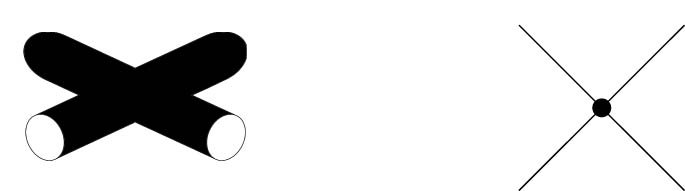
(Left) Singular crossing in a singular link, and (right) singular crossing in a singular link diagram.
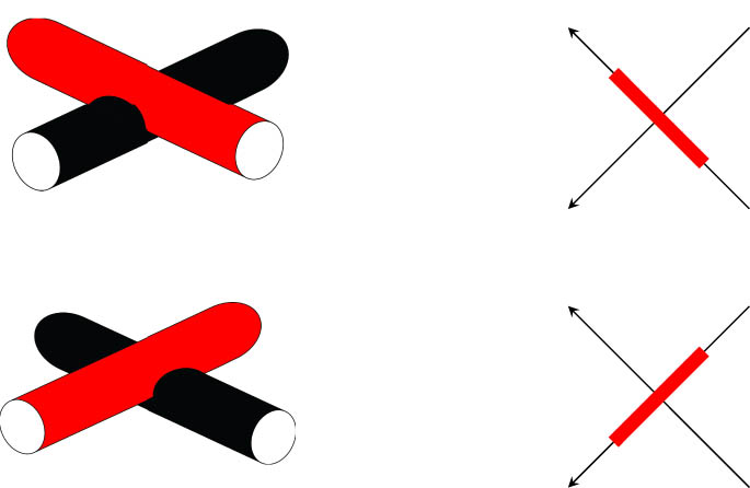
(Left) Stuck crossings in a stuck link, and (right) stuck crossings in a stuck link diagram.
To specify the stuck information in a diagram at a stuck crossing, we will use a thick bar on the over arc at a stuck crossing (Figure 2). The top crossings in Figure 2 are called positive stuck crossings, while the bottom crossings are negative stuck crossings.
In [2], the set of moves shown in Figure 3 was identified as a generating set of oriented stuck Reidemeister moves. We will follow the naming convention established in that paper. The oriented stuck Reidemeister moves are essential for studying stuck links through the use of stuck link diagrams. Specifically, two stuck link diagrams are equivalent if and only if one diagram can be transformed into the other by a finite sequence of planar isotopies and the moves in Figure 3. A stuck link is defined as an equivalence class of stuck link diagrams modulo the oriented stuck Reidemeister moves.
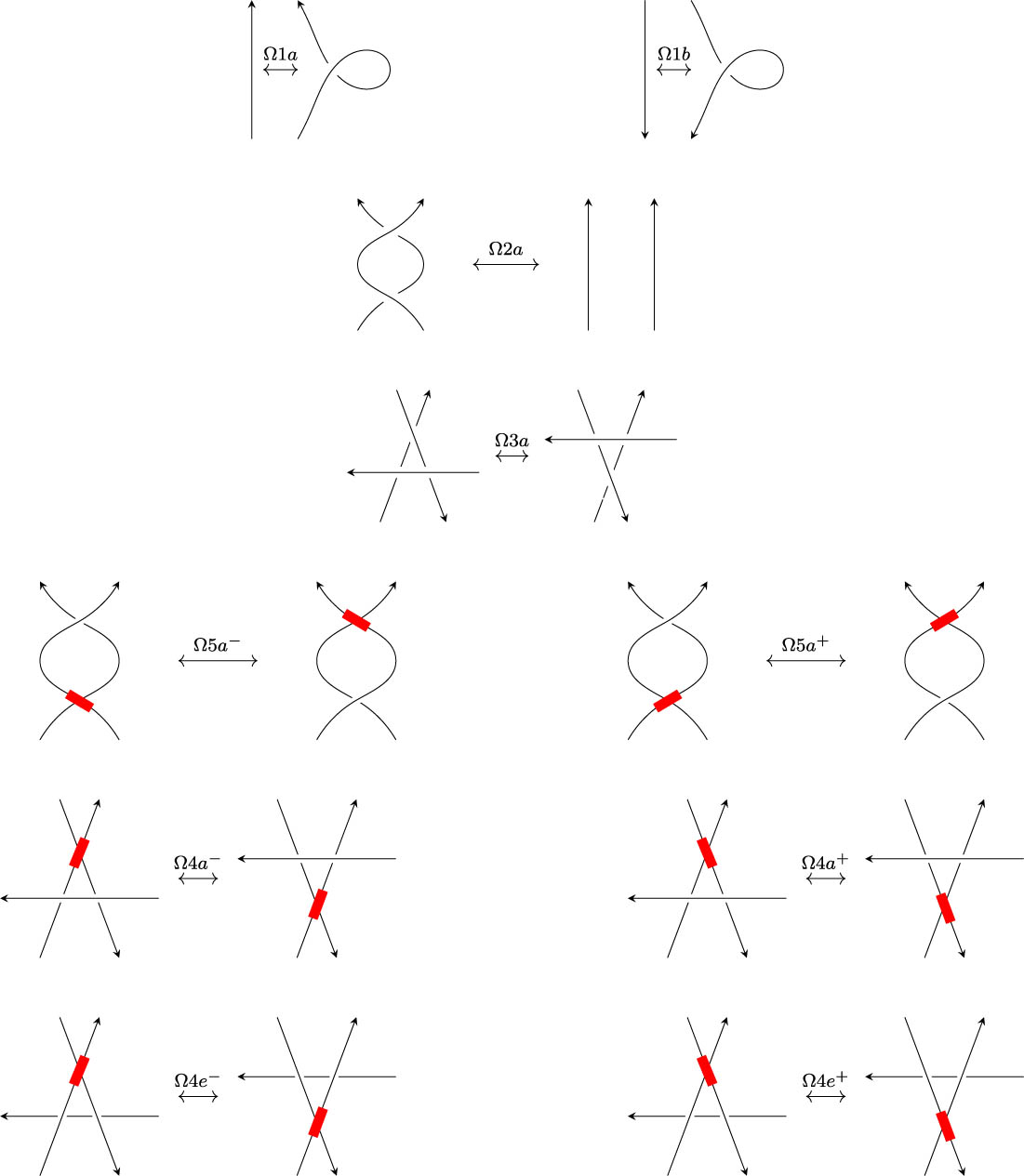
Generating set of oriented stuck Reidemeister moves.
3 Stuck links and arc diagrams
In this section, we review arc diagrams and the relationship between stuck links and arc diagrams. Specifically, stuck links provide a way of studying the topology of RNA folding, as discussed in [1–3].
In [10], Kauffmann and Magarshak introduced arc diagrams as a combinatorial way of studying the topology of RNA folding. Arc diagrams, as noted in [10], were motivated by the fact that the RNA molecule is a long chain consisting of the bases A (adenine), C (cytosine), U (uracil), and G (guanine). In an RNA molecule, the pairs A–U and C–G can bond with each other. Therefore, an RNA molecule can be represented by a linear sequence of the letters A, C, U, and G, and folding the molecule involves pairing the bases in the sequence. Example 3.1 is taken from [10].
Example 3.1
In this example, we will see how to obtain an arc diagram from the description of RNA folding as a linear sequence with pairings A–U and C–G. In this case, consider the chain
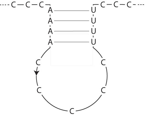
Folding of the sequence after the A-U pairing.
Arc diagram of the RNA folding in Figure 4.
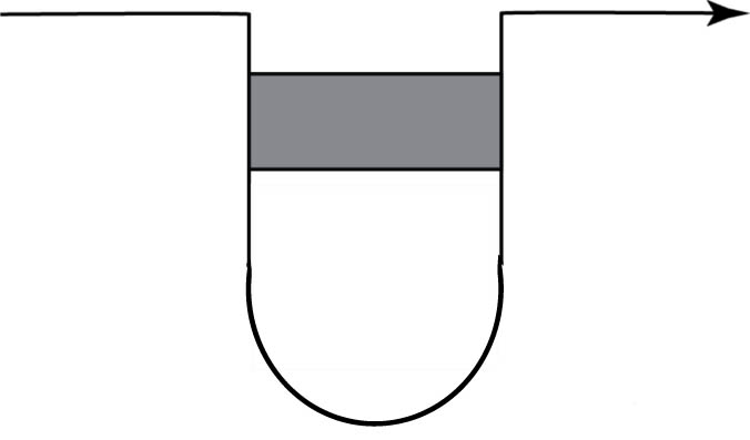
The diagram in Figure 5 is called an arc diagram introduced in [10]. We note that in the original formulation of an arc diagram, the bonds were denoted with connecting arcs. To see examples of these arc diagrams, please refer to [10]. In this article, we will use the convention introduced in [1] and used in [2,7] by replacing the connecting arcs with just one solid gray stripe, as shown in Figure 5. We also note that in order to study the topology of RNA folding in three-dimensional space through the use of an arc diagram, a set of Reidemeister-type moves was introduced in [10]. Therefore, a specific RNA folding is an equivalence class of arc diagrams modulo the Reidemeister-type moves. For more information on the Reidemeister-type moves allowed on an arc diagram and the theory of arc diagrams, please refer to [10].
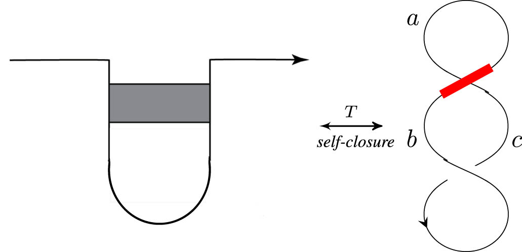
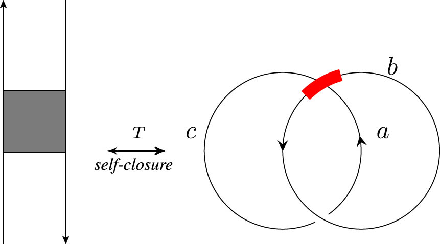
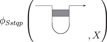
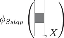
The following transformation was defined in [1] and formalizes the connection between stuck links and arc diagrams. To obtain a stuck link diagram from an arc diagram, we can apply the transformation,
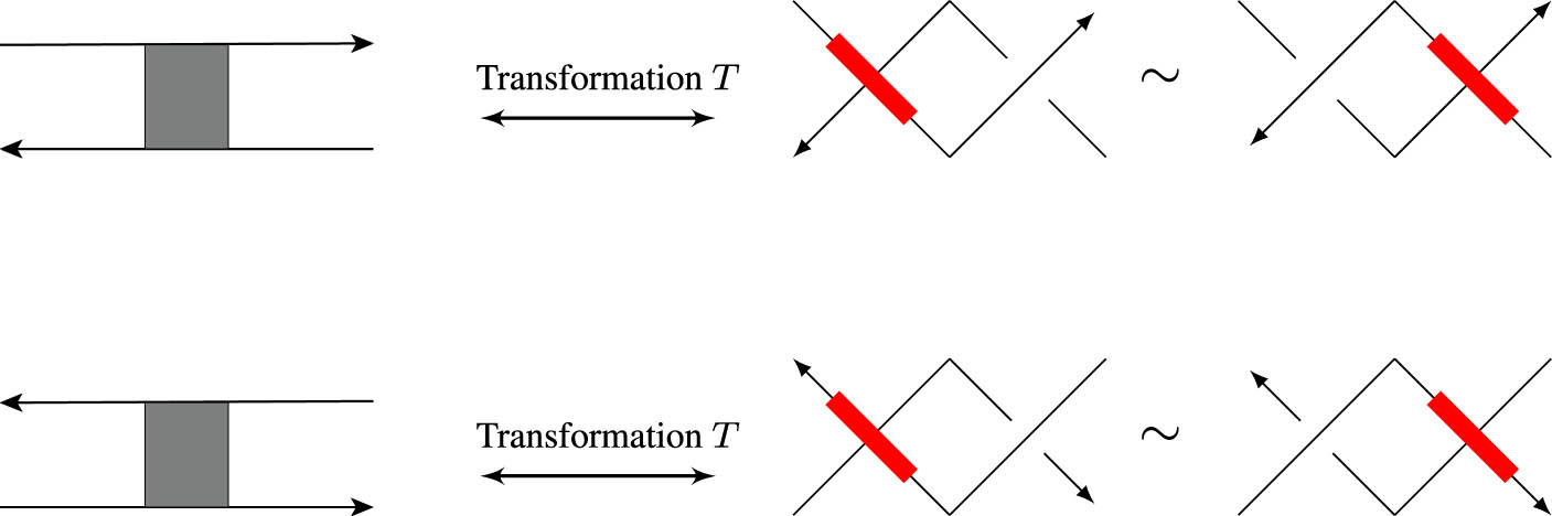
Transformation
In the following example, we will consider an arc diagram of an RNA folding and apply the transformation
Example 3.2
Consider the arc diagram of an RNA folding with two strands in Figure 7. In this case, the arc diagram contains two strands, so the self-closure means that we connect the endpoints of one strand to each other and the endpoints of the other strand to each other. Next, we replace the gray stripe by applying
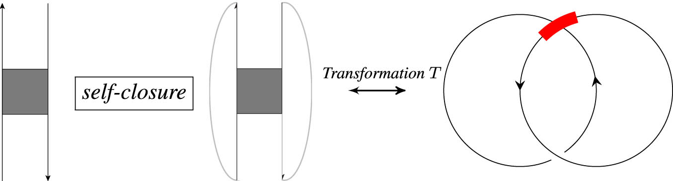
Arc diagram, self-closure, and corresponding stuck link diagram.
The transformation
4 Algebraic structures from stuck knots
In this section, we discuss the algebraic structures motivated by the diagrammatics of stuck knots and links. For more details on quandles, singquandles, and stuquandles, the reader is referred to [2,12,13].
The following definition is motivated by the Reidemeister moves in classical knot theory.
Definition 4.1
A quandle is a set
(right distributivity) for all
(invertibility) for all
(idempotency) for all
In the rest of the article, for all
Definition 4.2
Let
Definition 4.3
Let
Let
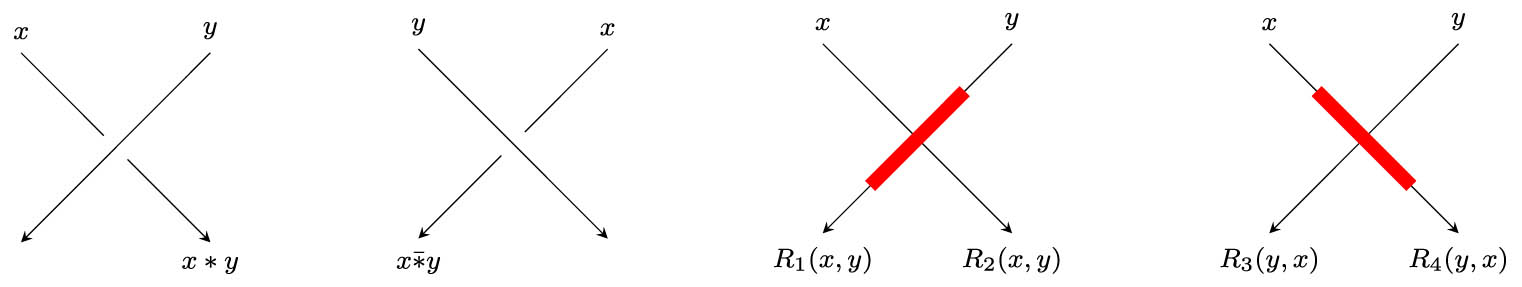
Coloring relations at classical and stuck crossings.
We note that the stuquandle axioms correspond to the oriented stuck Reidemeister moves, following the coloring rules in Figure 8. We will now review some key concepts about stuquandles, including basic examples.
Definition 4.4
Let
Definition 4.5
[2] Let
is called a stuquandle homomorphism. If, furthermore,
Lemma 4.6
Let
Proof
By definition, the image of
The following example was introduced in [2]. To see the construction details of the following stuquandle, the reader should refer to [2].
Example 4.7
Consider the set
Then, the six-tuple
Definition 4.8
[2] Let
The set of stuquandle words,
–
– If
The set
Let
The fundamental stuquandle of
In the following example, we use the notation and naming convention of stuck knots and links from [2].
Example 4.9
In this example, we compute the fundamental stuquandle of the following oriented stuck link. Consider the stuck trefoil, denoted by
We will label the arcs of the diagram

Diagram
The fundamental stuquandle can be used to define the following computable and effective invariant of stuck links. Given a finite stuquandle
We can think of each
5 Review of the quandle polynomial
In this section, we recall the definition of the quandle polynomial, the subquandle polynomial, and the link invariants obtained from the subquandle polynomial. For a detailed construction of these polynomials, see [8,12].
Definition 5.1
Let
and set
In [8], the quandle polynomial was shown to be an effective invariant of finite quandles. In addition to being an invariant of finite quandles, the quandle polynomial was generalized to give information about how a subquandle is embedded in a quandle.
Definition 5.2
Let
where
Note that for any knot or link
Definition 5.3
Let
Alternatively, the multiset can be represented in polynomial form by
6 Generalized quandle polynomials
In this section, we introduce a generalization of the quandle polynomial in [8]. We show that this generalization is an invariant of stuquandles. We then use the generalization to define a polynomial invariant of stuck links.
Definition 6.1
Let
Let
Proposition 6.2
If
Proof
Suppose
Definition 6.3
Let
Note that for
Example 6.4
Let
and the operations have the following
Thus, the stuquandle polynomial of
Next, consider the stuquandle
and the operations have the following
Thus, the stuquandle polynomial of
We obtain that
Example 6.5
Let
By Lemma 4.6, we know that the image of a stuquandle homomorphism is a substuquandle. Suppose that
Definition 6.6
Let
is the substuquandle polynomial invariant of L with respect to
7 Examples
In this section, we present examples that demonstrate the effectiveness of the substuquandle polynomial invariant in distinguishing stuck links. Specifically, we include an example that illustrates how the substuquandle polynomial invariant enhances the stuquandle counting invariant. Additionally, we include an example of two stuck links that are not distinguished by the
Example 7.1
Consider coloring the stuck knots
We collect the colorings of each stuck link and the substuquandle polynomial of the image of each coloring in Tables 1 and 2.
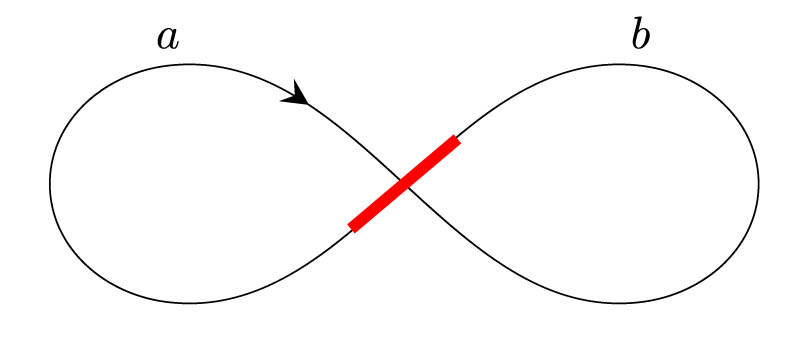
Diagram of the stuck knot
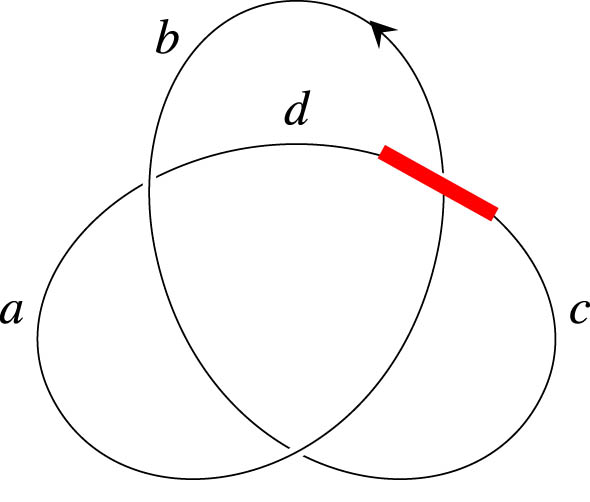
Diagram of the stuck trefoil
Colorings and substuquandle polynomial of each coloring of
|
|
|
|
|
|---|---|---|---|
| 0 | 0 |
|
|
| 0 | 2 |
|
|
| 2 | 0 |
|
|
| 2 | 2 |
|
|
Colorings and substuquandle polynomial of each coloring of
|
|
|
|
|
|
|
|---|---|---|---|---|---|
| 0 | 0 | 0 | 0 |
|
|
| 1 | 3 | 3 | 1 |
|
|
| 2 | 2 | 2 | 2 |
|
|
| 3 | 1 | 1 | 3 |
|
|
Using the coloring set of each stuck knot, we obtain the following substuquandle polynomial invariants:
and
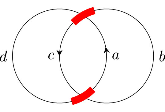
Diagram of the stuck link
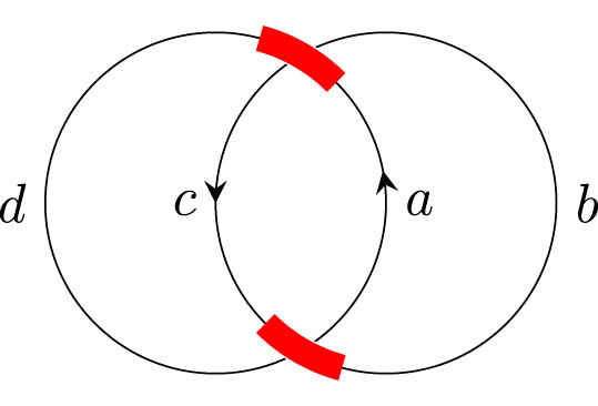
Diagram of the stuck link
Example 7.2
Consider coloring the stuck knots
The
and
Thus, the coloring invariant for both is 4. To calculate the substuquandle polynomial invariant of these stuck knots, we show in the tables below the operations have the following
We collect the colorings of each stuck link and the substuquandle polynomial of the image of each coloring in Tables 3 and 4.
Using the coloring set of each stuck link, we obtain the following substuquandle polynomial invariants:
and
which shows that our invariant is stronger than the
Colorings and substuquandle polynomial of each coloring of
|
|
|
|
|
|
|
|---|---|---|---|---|---|
| 0 | 0 | 0 | 0 |
|
|
| 1 | 0 | 1 | 0 |
|
|
| 0 | 1 | 0 | 1 |
|
|
| 1 | 1 | 1 | 1 |
|
|
Colorings and substuquandle polynomial of each coloring of
|
|
|
|
|
|
|
|---|---|---|---|---|---|
| 0 | 0 | 0 | 0 |
|
|
| 0 | 2 | 0 | 2 |
|
|
| 2 | 0 | 2 | 0 |
|
|
| 2 | 2 | 2 | 2 |
|
|
Now we will compute our new substuquandle polynomial invariant to distinguish the topology of RNA structure. First, we will consider an arc diagram of RNA folding, then use the transformation
Example 7.3
Let
We will consider the two arc diagrams of RNA foldings and their corresponding stuck links (Figures 14 and 15).
With respect to the stuquandle defined above, the colorings for Figure 14 are
We collect the colorings of each arc diagram and the substuquandle polynomial of the image of each coloring in Tables 5 and 6. Using the coloring set of each arc diagram, we obtain the following substuquandle polynomial invariants:
Arc diagram and corresponding stuck link
Arc diagram and corresponding stuck link diagram denoted by
Colorings and substuquandle polynomial of each coloring of
|
|
|
|
|
|
|---|---|---|---|---|
| 0 | 0 | 0 |
|
|
| 1 | 3 | 3 |
|
|
| 2 | 2 | 2 |
|
|
| 3 | 1 | 1 |
|
|
Colorings and substuquandle polynomial of each coloring of
|
|
|
|
|
|
|---|---|---|---|---|
| 0 | 0 | 0 |
|
|
| 0 | 2 | 0 |
|
|
| 2 | 0 | 2 |
|
|
| 2 | 2 | 2 |
|
|
and
Thus, the RNA foldings are distinguished since
Acknowledgments
The authors would like to thank the referee for the fruitful comments, which improved the article.
-
Funding information: Mohamed Elhamdadi was partially supported by Simons Foundation collaboration grant 712462.
-
Author contributions: All authors contributed equally. All authors have accepted responsibility for the entire content of this manuscript and consented to its submission to the journal, reviewed all the results, and approved the final version of the manuscript.
-
Conflict of interest: Prof. Mohamed Elhamdadi is an Editor of the Open Mathematics journal and was not involved in the review and decision-making process of this article.
References
[1] K. Bataineh, Stuck knots, Symmetry 12 (2020), no. 9, 1558. 10.3390/sym12091558Suche in Google Scholar
[2] J. Ceniceros, M. Elhamdadi, J. Komissar, and H. Lahrani, RNA foldings and stuck knots, Commun. Korean Math. Soc. 39 (2024), no. 1, 223–245. Suche in Google Scholar
[3] J. Ceniceros, M. Elhamdadi, B. Magill, and G. Rosario, RNA foldings, oriented stuck knots, and state sum invariants, J. Math. Phys. 64 (2023), no. 3, 031702.10.1063/5.0140652Suche in Google Scholar
[4] A. S. Crans, S. Nelson, and A. Sarkar, Enhancements of rack counting invariants via dynamical cocycles, New York J. Math. 18 (2012), 337–351. Suche in Google Scholar
[5] J. S. Carter, D. Jelsovsky, S. Kamada, L. Langford, and M. Saito, Quandle cohomology and state-sum invariants of knotted curves and surfaces, Trans. Amer. Math. Soc. 355 (2003), no. 10, 3947–3989. 10.1090/S0002-9947-03-03046-0Suche in Google Scholar
[6] J. S. Carter, M. Elhamdadi, and M. Saito, Homology theory for the set-theoretic Yang-Baxter equation and knot invariants from generalizations of quandles, Fund. Math. 184 (2004), 31–54. 10.4064/fm184-0-3Suche in Google Scholar
[7] J. S. Carter, M. Elhamdadi, M. Grannna, and M. Saito, Cocycle knot invariants from quandle modules and generalized quandle homology, Osaka J. Math. 42 (2005), no. 3, 499–541. Suche in Google Scholar
[8] S. Nelson, Generalized quandle polynomials, Canad. Math. Bull. 54 (2011), no. 1, 147–158. 10.4153/CMB-2010-090-xSuche in Google Scholar
[9] J. Ceniceros, I. R. Churchill, and M. Elhamdadi, Polynomial invariants of singular knots and links, J. Knot Theory Ramifications 30 (2021), no. 1, 2150003.10.1142/S0218216521500036Suche in Google Scholar
[10] L. H. Kauffman and Y. B. Magarshak, Vassiliev knot invariants and the structure of RNA folding, Knots and Applications Series on Knots and Everything, vol. 6, World Scientific Publishing, River Edge, NJ, 1995, pp. 343–394. 10.1142/9789812796189_0009Suche in Google Scholar
[11] W. Tian, X. Lei, L. H. Kauffman, and J. Liang, A knot polynomial invariant for analysis of topology of RNA stems and protein disulfide bonds, Mol. Based Math. Biol. 5 (2017), 21–30. 10.1515/mlbmb-2017-0002Suche in Google Scholar PubMed PubMed Central
[12] M. Elhamdadi and S. Nelson, Quandles–an introduction to the algebra of knots, Student Mathematical Library, vol. 74, American Mathematical Society, Providence, RI, 2015. 10.1090/stml/074Suche in Google Scholar
[13] K. Bataineh, M. Elhamdadi, M. Hajij, and W. Youmans, Generating sets of Reidemeister moves of oriented singular links and quandles, J. Knot Theory Ramifications 27 (2018), no. 14, 1850064. 10.1142/S0218216518500645Suche in Google Scholar
© 2025 the author(s), published by De Gruyter
This work is licensed under the Creative Commons Attribution 4.0 International License.
Artikel in diesem Heft
- On I-convergence of nets of functions in fuzzy metric spaces
- Special Issue on Contemporary Developments in Graphs Defined on Algebraic Structures
- Forbidden subgraphs of TI-power graphs of finite groups
- Finite group with some c#-normal and S-quasinormally embedded subgroups
- Classifying cubic symmetric graphs of order 88p and 88p 2
- Two-sided zero-divisor graphs of orientation-preserving and order-decreasing transformation semigroups
- Simplicial complexes defined on groups
- Further results on permanents of Laplacian matrices of trees
- Algebra
- Classes of modules closed under projective covers
- On the dimension of the algebraic sum of subspaces
- Green's graphs of a semigroup
- On an uncertainty principle for small index subgroups of finite fields
- On a generalization of I-regularity
- Algorithm and linear convergence of the H-spectral radius of weakly irreducible quasi-positive tensors
- The hyperbolic CS decomposition of tensors based on the C-product
- On weakly classical 1-absorbing prime submodules
- Equational characterizations for some subclasses of domains
- Algebraic Geometry
- Spin(8, ℂ)-Higgs bundles fixed points through spectral data
- Embedding of lattices and K3-covers of an Enriques surface
- Kodaira-Spencer maps for elliptic orbispheres as isomorphisms of Frobenius algebras
- Applications in Computer and Information Sciences
- Dynamics of particulate emissions in the presence of autonomous vehicles
- Exploring homotopy with hyperspherical tracking to find complex roots with application to electrical circuits
- Category Theory
- The higher mapping cone axiom
- Combinatorics and Graph Theory
- 𝕮-inverse of graphs and mixed graphs
- On the spectral radius and energy of the degree distance matrix of a connected graph
- Some new bounds on resolvent energy of a graph
- Coloring the vertices of a graph with mutual-visibility property
- Ring graph induced by a ring endomorphism
- A note on the edge general position number of cactus graphs
- Complex Analysis
- Some results on value distribution concerning Hayman's alternative
- Freely quasiconformal and locally weakly quasisymmetric mappings in metric spaces
- A new result for entire functions and their shifts with two shared values
- On a subclass of multivalent functions defined by generalized multiplier transformation
- Singular direction of meromorphic functions with finite logarithmic order
- Growth theorems and coefficient bounds for g-starlike mappings of complex order λ
- Refinements of inequalities on extremal problems of polynomials
- Control Theory and Optimization
- Averaging method in optimal control problems for integro-differential equations
- On superstability of derivations in Banach algebras
- The robust isolated calmness of spectral norm regularized convex matrix optimization problems
- Observability on the classes of non-nilpotent solvable three-dimensional Lie groups
- Differential Equations
- The ill-posedness of the (non-)periodic traveling wave solution for the deformed continuous Heisenberg spin equation
- A note on the global existence and boundedness of an N-dimensional parabolic-elliptic predator-prey system with indirect pursuit-evasion interaction
- Blow-up of solutions for Euler-Bernoulli equation with nonlinear time delay
- Periodic or homoclinic orbit bifurcated from a heteroclinic loop for high-dimensional systems
- Regularity of weak solutions to the 3D stationary tropical climate model
- Local minimizers for the NLS equation with localized nonlinearity on noncompact metric graphs
- Global existence and blow-up of solutions to pseudo-parabolic equation for Baouendi-Grushin operator
- Bubbles clustered inside for almost-critical problems
- Existence and multiplicity of positive solutions for multiparameter periodic systems
- Existence of positive periodic solutions for evolution equations with delay in ordered Banach spaces
- On a nonlinear boundary value problems with impulse action
- Normalized ground-states for the Sobolev critical Kirchhoff equation with at least mass critical growth
- Multiple positive solutions to a p-Kirchhoff equation with logarithmic terms and concave terms
- Infinitely many solutions for a class of Kirchhoff-type equations
- Real and non-real eigenvalues of regular indefinite Sturm–Liouville problems
- Existence of global solutions to a semilinear thermoelastic system in three dimensions
- Limiting profile of positive solutions to heterogeneous elliptic BVPs with nonlinear flux decaying to negative infinity on a portion of the boundary
- Morse index of circular solutions for repulsive central force problems on surfaces
- Differential Geometry
- On tangent bundles of Walker four-manifolds
- Pedal and negative pedal surfaces of framed curves in the Euclidean 3-space
- Discrete Mathematics
- Eventually monotonic solutions of the generalized Fibonacci equations
- Dynamical Systems Ergodic Theory
- Dynamical properties of two-diffusion SIR epidemic model with Markovian switching
- A note on weighted measure-theoretic pressure
- Pullback attractors for a class of second-order delay evolution equations with dispersive and dissipative terms on unbounded domain
- Pullback attractor of the 2D non-autonomous magneto-micropolar fluid equations
- Functional Analysis
- Spectrum boundary domination of semiregularities in Banach algebras
- Approximate multi-Cauchy mappings on certain groupoids
- Investigating the modified UO-iteration process in Banach spaces by a digraph
- Tilings, sub-tilings, and spectral sets on p-adic space
- Continuity and essential norm of operators defined by infinite tridiagonal matrices in weighted Orlicz and l∞ spaces
-
A family of commuting contraction semigroups on
- q-Stirling sequence spaces associated with q-Bell numbers
- Chlodowsky variant of Bernstein-type operators on the domain
- Hyponormality on a weighted Bergman space of an annulus with a general harmonic symbol
- Characterization of derivations on strongly double triangle subspace lattice algebras by local actions
- Fixed point approaches to the stability of Jensen’s functional equation
- Geometry
- The regularity of solutions to the Lp Gauss image problem
- Solving the quartic by conics
- Group Theory
- On a question of permutation groups acting on the power set
- A characterization of the translational hull of a weakly type B semigroup with E-properties
- Harmonic Analysis
- Eigenfunctions on an infinite Schrödinger network
- Maximal function and generalized fractional integral operators on the weighted Orlicz-Lorentz-Morrey spaces
- Subharmonic functions and associated measures in ℝn
- Mathematical Logic, Model Theory and Foundation
- A topology related to implication and upsets on a bounded BCK-algebra
- Boundedness of fractional sublinear operators on weighted grand Herz-Morrey spaces with variable exponents
- Number Theory
- Fibonacci vector and matrix p-norms
- Recurrence for probabilistic extension of Dowling polynomials
- Carmichael numbers composed of Piatetski-Shapiro primes in Beatty sequences
- The number of rational points of some classes of algebraic varieties over finite fields
- Classification and irreducibility of a class of integer polynomials
- Decompositions of the extended Selberg class functions
- Joint approximation of analytic functions by the shifts of Hurwitz zeta-functions in short intervals
- Fibonacci Cartan and Lucas Cartan numbers
- Recurrence relations satisfied by some arithmetic groups
- The hybrid power mean involving the Kloosterman sums and Dedekind sums
- Numerical Methods
- A modified predictor–corrector scheme with graded mesh for numerical solutions of nonlinear Ψ-caputo fractional-order systems
- A kind of univariate improved Shepard-Euler operators
- Probability and Statistics
- Statistical inference and data analysis of the record-based transmuted Burr X model
- Multiple G-Stratonovich integral in G-expectation space
- p-variation and Chung's LIL of sub-bifractional Brownian motion and applications
- Real Analysis
- Chebyshev polynomials of the first kind and the univariate Lommel function: Integral representations
- Multiple solutions for a class of fourth-order elliptic equations with critical growth
- Majorization-type inequalities for (m, M, ψ)-convex functions with applications
- The evaluation of a definite integral by the method of brackets illustrating its flexibility
- Some new Fejér type inequalities for (h, g; α - m)-convex functions
- Some new Hermite-Hadamard type inequalities for product of strongly h-convex functions on ellipsoids and balls
- Topology
- Unraveling chaos: A topological analysis of simplicial homology groups and their foldings
- A generalized fixed-point theorem for set-valued mappings in b-metric spaces
- On SI2-convergence in T0-spaces
- Generalized quandle polynomials and their applications to stuquandles, stuck links, and RNA folding