Hybrid deep learning for bankruptcy prediction: An optimized LSTM model with harmony search algorithm

Mohamed Elhoseny; Saadat M. Alhashmi; Mohanad A. Deif; Rhada Boujlil; Noura Metawa

doi:10.1515/jisys-2025-0058

Artikel Open Access

Hybrid deep learning for bankruptcy prediction: An optimized LSTM model with harmony search algorithm

Mohamed Elhoseny , Saadat M. Alhashmi , Mohanad A. Deif , Rhada Boujlil und Noura Metawa

Veröffentlicht/Copyright: 5. September 2025

Veröffentlicht von

Veröffentlichen auch Sie bei De Gruyter Brill

Manuskript einreichen Informationen für Autor*innen

Aus der Zeitschrift Journal of Intelligent Systems Band 34 Heft 1

Abstract

Accurate bankruptcy prediction is essential for financial stability, risk management, and decision making. Traditional statistical models cannot capture complex nonlinear relationships in financial data; hence, it is essential to use advanced deep learning techniques. This study proposes a hybrid long short-term memory (LSTM) model, optimized using the harmony search algorithm (HSA) for enhanced predictability. A financial dataset of Polish companies from the emerging markets information service was utilized, which consisted of financial indicators spanning several years. For feature selection, principal component analysis was employed to achieve dimensionality reduction without loss of pertinent financial data. The new HSA-LSTM model was compared with benchmark classifiers such as fuzzy logic neural network, kernel extreme learning machine, extreme learning machine, and support vector machine in terms of key performance measures. The HSA-LSTM model outperformed all of the baselines with 90.80% accuracy, 89.46% precision, 90.22% recall, and an F-score of 90.54%. Statistical verification using ANOVA and Tukey’s HSD test confirmed that the improvement was significant (p < 0.05). These findings highlight deep learning with hyperparameter optimization for financial distress prediction. This study contributes to early bankruptcy prediction and financial risk modeling and offers a high-accuracy, scalable prediction model. Future research could explore additional metaheuristic optimization techniques, explainable AI (XAI), and macroeconomic indicators to further enhance predictive accuracy.

Keywords: deep learning; artificial intelligence; bankruptcy prediction; financial risk management; metaheuristic optimization

1 Introduction

Corporate bankruptcy forecasting matters to investors, corporate executives, policymakers, and finance analysts [1,2]. Bankruptcy forecasting models help to mitigate the risks to finance through early indicators of financial distress that enable interventions to be made proactively [3]. The complexity of global markets and volatility of the economy have created the need for robust models to predict financial distress that can effectively discriminate between solvent and insolvent firms. Logistic regression (LR) and discriminant analysis (DA) are standard statistical models that have been employed to predict bankruptcy but are likely to fail to capture the nonlinearities and temporal dynamics within financial data. Consequently, complex machine-learning algorithms have been increasingly used to enhance the accuracy of financial distress forecasts.

Financial distress [4,5] is an intricate issue that arises based on numerous economic, operational, and market-related factors. Financially distressed firms are commonly characterized by downward-trending profitability, increasing liabilities, reduced liquidity, and poor operational efficacy. Such measures are obtained from financial reports and predicted using predictive models to ascertain the possibility of a firm becoming insolvent. The database employed in this study includes the financial reports of Polish firms obtained from the Emerging Markets Information Service (EMIS), bankrupt firms, and non-bankrupt firms for a series of years. The employment of financial measures such as profitability ratios, measures of liquidity, leverage ratios, and measures of asset efficiency completes the analysis. With the multidimensional nature of the financial information, the employment of techniques such as principal component analysis (PCA) [6,7] has gained extensive use to prevent redundancy but preserve the most informative features to be used for classification.

New advances in deep learning [8] have exhibited superior performance in the modeling of complex temporal relationships within finance datasets. Recurrent neural networks (RNNs), particularly long short-term memory (LSTM) [9] networks, have gained popularity in finance modeling due to the ability to preserve information within the networks through extended sequences. LSTM networks address the vanishing gradient problem that has been witnessed within traditional RNNs for use in time-series analysis within finance. Nevertheless, the issue of hyperparameter tuning continues to be an impediment to the optimization of LSTM-based models for predicting bankruptcy. This limitation has been reduced using metaheuristic optimization algorithms such as the harmony search algorithm (HSA) [10] to LSTM networks to further the predictive ability through optimization of the learning rate, dropout rate, and the LSTM units.

This study introduces an HSA-LSTM model to be employed in the prediction of bankruptcy based on the strengths of LSTM to address sequential financial data and the employment of HSA to tune the hyperparameters.

The HSA was selected for hyperparameter tuning because of its simplicity, efficiency, and strong global search capability. Unlike gradient-based methods, HSA avoids local minima by stochastically generating new solutions and updating harmony memory based on fitness. Its musical improvisation analogy enables flexibility in exploring the search space, making it particularly suitable for optimizing deep learning models, such as LSTM, which are sensitive to initial hyperparameter choices. The proposed model was also compared with conventional classifiers, that is, the fuzzy logic neural network (FLNN), kernel extreme learning machine (KELM), extreme learning machine (ELM), and support vector machine (SVM). The performance was analyzed using key classification metrics, that is, precision, recall, accuracy, and F-score, to provide an overall picture of the model’s predictive capability.

Machine learning algorithms have been shown to be efficient substitutes for conventional algorithms with greater flexibility and sensitivity in the field of financial prediction. Ensemble learning algorithms, SVMs, and decision trees have been quickly applied to forecast financial distress [3]. Deep learning models derived from LSTM models have been used in recent studies, with encouraging results in bankruptcy prediction, as LSTM models can detect long-term trends in financial data. LSTM networks are distinct from standard feedforward neural networks owing to the introduction of gateway mechanisms that regulate information flow, enabling the networks to extract temporal relationships from sequential financial statements spanning a period of many years [4].

Despite advancements in deep-learning-based financial distress prediction, some challenges remain. The imbalance in bankruptcy datasets, where the number of non-bankrupt firms greatly outnumbers that of bankrupt firms, is a major hindrance to model training. Conventional classification algorithms are biased toward the majority class and yield unsatisfactory predictions for financially distressed firms. In addition, the selection of pertinent financial indicators and hyperparameter tuning is crucial for ascertaining model performance. Addressing these challenges requires a hybrid approach that combines feature selection, hyperparameter optimization, and advanced classification techniques to enhance the predictive accuracy.

PCA is employed in this study to reduce the dimensionality of the financial indicators but maintain important information to be employed within the classification. A new approach to forecasting bankruptcy is presented by using the HSA-LSTM model, which employs the HSA to optimize the model’s hyperparameters to improve its efficacy. The performance of the new model under different forecasting horizons was used to ascertain how it predicted financial distress within different intervals to the time of bankruptcy. Using sequential finance data and metaheuristic optimization, this study attempts to enhance the reliability and accuracy of the models employed to predict bankruptcy.

The remainder of this article is organized as follows. Section 2 provides related work through an overview of the literature regarding the models used to predict bankruptcy and the recent literature on forecasting financial distress using deep learning. Section 3 provides the methodology through the presentation of the dataset used, selection of the features used, and classification models used. Section 4 provides the results of the analysis of the performance of the models using primary measures. Section 5 discusses the implications of the proposed model in forecasting financial distress. Section 6 concludes the article by presenting future research recommendations.

2 Related work

Corporate bankruptcy and financial crisis forecasting have been the subject of extensive research, evolving from linear statistical models to sophisticated machine learning and deep learning methodologies. Early models such as LR and DA made linear assumptions about the relationship between financial indicators and the likelihood of bankruptcy, constraining precision. The complexity of the financial market has made nonlinear models more essential, especially the use of deep learning models that have proven to be more efficient in extracting temporal relationships and factor interactions within financial information.

Many studies have explored the application of deep-learning models to predict financial crises. Pang and Du [11] introduced an LSTM model that was optimized using the whale optimization algorithm to predict SME financial distress. The model achieved an accuracy rate of 97.5% based on 13 crucial financial indicators in five aspects to significantly improve the forecasting capability. Zhao [12] designed a hybrid model that fused artificial bee colony-recurrent neural network and bidirectional LSTM (Bi-LSTM), optimizing the weights selection process to achieve a 93.8% recall. Tang [13] similarly employed the combination of convolutional neural networks (CNN) and LSTM to employ both structured financial ratios and textual information from the financial reports to improve the precision of the financial risk analysis by 12.5% over isolated models.

The application of optimization algorithms to forecast financial distress has been studied to a large degree to enhance accuracy. Li and Chen [14] introduced an improved fruit fly optimization algorithm-backpropagation neural network that optimizes the model weights to evade the issue of the local minimum. The proposed model achieved a mean squared error of 2.31, a mean absolute error of 1.48, and a mean absolute percentage error of 3.92%, which were better than those of the ACO-BP, particle swarm optimization-backpropagation, and standard fruit fly optimization models. Guo [15] employed a genetic algorithm-least-squares support vector machine technique to raise the accuracy of the classification of financial distress to 91.2% from 84.7%. Kalaivani [16], similarly, employed the chimp optimization algorithm to optimize the KELM models to an accuracy of 94.01%, which was far superior to the standard machine learning models such as SVM and random forest (RF).

Hybrid machine learning models have also been employed to address financial risk forecasting. Abdul-Kareem et al. [17] hybridized XGBoost with PSO to reduce the feature space by 30% but preserve 100% classification accuracy for financial distress. Purnell [18] hybridized PSO with SVM to optimize the indicators of financial risks to achieve an 11.5% improvement in classification precision over the traditional SVM models. Jian and Yu [19] used the optimization of the parameters of SVM through grey wolf optimization to achieve an accuracy rate of 94.3% using the financial crisis datasets.

Feature selection algorithms and explainable AI (XAI) methodologies were presented to enable model interpretability and efficiency. Quan et al. [20] presented a method of variable selection that employed the use of Shapley values along with modified Borda counts to effectively reduce financial distress prediction variables to 14 from 3,160 and enhance classification to 92.6%. Torky et al. [21] presented an explainable machine learning model that employed the use of pigeon optimization along with a gradient boosting classifier that achieved 99% training accuracy and 96.7% test accuracy. The increasing application of XAI methodologies emphasizes the need to design highly accurate financial distress prediction models; however, they are also transparent about the decision process.

Another region that has experienced integration is the application of macroeconomic indicators in models of forecasting financial crises. Chen et al. [22] employed RF and XGBoost on stock market information to increase the accuracy of forecasting financial crises by 9.4% from the use of standard models. Tan et al. [23] designed an index of China’s financial stability based on a Markov regime switching model and XGBoost to classify the degrees of the risks to be high, medium, and low regimes, having an 89.8% accuracy. The application of macroeconomic indicators enhances forecasting models by identifying larger economic conditions that determine the financial stability of businesses.

Current advances in big data analysis have also contributed to forecasting financial distress. Zhang et al. [24] designed an early warning system using big data that included both financial and non-financial information using a multi-dimensional logistic model to gain a 15.3% improvement in the identification accuracy of crises. Qiang [25] employed supervised learning to predict banking crises within the African economies using a two-layer neural network using the ReLU activation function to raise the reliability of forecasting financial crises to 21.6%. Also, Zhang et al. [26] examined the contribution made by external financial shocks to cause corporate insolvency using ensemble learning algorithms to gain an F-score of 91.4% in firm bankruptcy forecasting.

Growing research has focused on enhancing the robustness of models of financial distress using alternative methodologies. Ju and Zhu [27] suggested a reinforcement learning-based finance risk model that dynamically adjusted the weights of the characteristics based upon real-time market dynamics to improve the stability of the forecasts by 13.2%. Li et al. [28] looked at the use of transfer learning to address the issue of forecasting bankruptcy through the transfer of pre-trained models to new marketplaces to decrease the models’ training time by 10.6% but maintain high precision.

Other studies have attempted to improve the prediction of financial crises by using ensemble learning techniques. Feng et al. [29] employed a stacking ensemble technique that incorporated the use of decision trees, SVM, and RF classifier models to achieve 95.2% classification. Torky et al. [21] employed an Adaptive Boosting (AdaBoost) framework to lower the percentage of false positives by 14.5%. Finally, Zhao [30] explored the use of Bayesian neural networks to measure financial risks with an 8.1% greater precision than the use of traditional deep learning models.

The literature on the forecasting of financial distress continues to be innovative in the application of deep learning, optimization algorithms, feature selection, and hybrid modeling. While LSTM, CNN, and Bi-LSTM deep learning models have proven to be successful, recent studies emphasize the necessity of coupling explainability, macroeconomic data, and ensemble learning techniques to further improve the precision of the models. The future will be steered toward real-time forecasting, greater model explainability, and the integration of non-conventional sources of data, such as social media sentiment analysis and trends, to produce a more comprehensive framework to measure risks.

3 Problem statement and main contributions of the study

Corporate bankruptcy forecasting remains a crucial issue in the field of financial risk management and has a direct impact on stakeholders such as investors, lenders, policymakers, and managers. The ability to accurately forecast financial distress makes early decision-making possible, which constrains financial losses and preserves economic stability. The models currently employed to forecast bankruptcy suffer from issues such as data complexity, unbalanced datasets, feature selection, and model optimization. Traditional statistical models such as LR and DA are founded upon the linear relationship between finance indicators and bankruptcy risk, but are suboptimal under real-world conditions where the determinants of financial distress are non-linear and dynamically interactive. Machine learning models such as SVM, decision trees, and ELM have proven to be superior at making forecasts, but are typically accompanied by the need to perform extensive feature engineering and hyperparameter optimization to produce maximum performance.

A primary limitation in the prediction of financial distress comes from the large dimensionality of financial information and the existence of irrelevant or redundant financial indicators that can lower the precision of the models. In addition, the unbalanced nature of bankruptcy datasets, where bankrupt companies form a minority within the entire dataset, causes classification algorithms to be biased toward financially healthy companies. Although deep learning models, such as LSTM networks, have been proposed to deal with the sequential nature of financial reports, they are highly reliant upon tuning the hyperparameters that are computationally expensive and require expertise. Consequently, there is a necessity to create a hybrid framework that combines the use of feature selection, the optimization of hyperparameters, and the use of deep learning models to improve the precision of bankruptcy prediction but avoid computational inefficiencies.

This study addresses the challenges outlined above through the proposal of an HSA-LSTM model that blends the HSA to tune the hyperparameter with LSTM networks to be employed in the forecasting of financial distress. The main contributions of this study are as follows:

This study introduces a new HSA-LSTM model that capitalizes on the sequence learning capability of LSTM networks, but relies on HSA to optimize the hyperparameters. The technique optimizes crucial parameters such as the learning rate, batch size, drop rate, and number of LSTM units to enhance the predictive accuracy.
PCA was employed to resolve the issue of large-dimensional financial information to eliminate redundancy and maintain the most influential financial indicators. This enhances computational efficiency, retaining only the most informative financial characteristics responsible for the classification.
The new model was compared with machine learning and other traditional classifiers, such as FLNN, KELM, ELM, and SVM. This comparison provides an understanding of the comparative effectiveness of the different classification techniques employed to forecast bankruptcy.
This study measures the performance of the models along a sequence of forecasting horizons from 1 to 5 years to the date of bankruptcy. This provides an extensive analysis of the model’s ability to predict financial distress within various periods to aid early warning systems.
We conducted a one-way ANOVA to determine the statistical difference in the performance of the models to ascertain the reliability of the findings, and then employed Tukey’s HSD post-hoc test to ascertain the difference that is significant between models. Statistical tests confirm the reliability of the proposed method.
This research draws upon a large database of Polish firms sourced from the EMIS, which contains the financial information of bankrupt and non-failed firms across several years. The database contains 64 financial measures, including profitability, liquidity, leverage, and asset efficiency, providing a real-world analysis of the forecasting of financial distress within an emerging market.

By combining metaheuristic optimization, statistical validation techniques, and deep learning, this study presents a comprehensive and efficient framework for forecasting bankruptcy. The study proves the feasibility of the use of LSTM models in finance forecasting and presents the necessity of tuning the hyperparameters to improve forecasting accuracy. The proposed HSA-LSTM model outperforms the baseline classifier models, providing a practical method to be employed in real-world finance risk analysis, credit analysis, and firm decision-making.

4 Methodology and materials

4.1 Materials

The database utilized for this study comprises financial data of Polish firms [31] that are either currently in business or have failed within a specified time frame. The data were collected from the EMIS [31], which is a comprehensive database that offers financial data related to emerging markets, macroeconomic, and industry data associated with Poland. EMIS offers access to more than 510 publications covering structured financial issue data, stock market trend data, company reports, and macroeconomic data. The database is useful as a suitable vehicle for research with the aim of predicting financial distress.

The time frame covered by the dataset varies from 2007 to 2013 for bankrupt entities and from 2000 to 2012 for non-bankrupt entities. Temporal differences were based on the availability of financial records within the EMIS database. The sample is an unbalanced dataset that includes bankrupt entities, as well as entities that remain operational. Specifically, we used the financial records of 707 bankrupt entities (equivalent to approximately 2,100 records). The financial information of over 10,000 non-bankrupt entities was also included within the dataset to ensure that financially viable entities were represented sufficiently. To ensure the reliability of the analysis, entities that went bankrupt but did not leave complete financial records were excluded, giving a dataset of more than 65,000 records. The selection and organization methods used to generate the training dataset are listed in Table 1, where the criteria and sources used to compile the information are given.

Table 1

Methodology of collecting the training data

Name	Criterion	Selection details
Sector	The largest number of bankruptcies in the sector compared to the others	The manufacturing sector in Poland was chosen
Database of financial statements	The availability of financial statements	The EMIS database was used, covering bankrupt and operating firms
Bankrupt companies	Availability of at least one financial statement for each bankrupt company	707 bankrupt firms from 2007 to 2013 were included
Still operating companies	The availability of financial statements for a non-bankrupt company during the period 2000–2012	More than 10,000 non-bankrupt firms were included
Financial indicators	Indicators used in previous research for financial distress prediction	64 financial indicators were selected for the analysis

To facilitate the classification tasks, financial data were segmented into five different forecasting periods, each representing a different time horizon for bankruptcy prediction. The forecasting periods are described in detail as follows.

First Year: Contains financial ratios from the year preceding bankruptcy, with corresponding class labels indicating bankruptcy status after 1 year. The dataset includes 7,792 financial records of 1,057 bankrupt firms and 6,735 non-bankrupt firms.
Second Year: Contains financial data from 2 years before bankruptcy. The dataset consists of 10,173 financial records, with 400 bankrupt firms and 9,773 non-bankrupt firms.
Third Year: Financial indicators from 3 years prior to bankruptcy are included, with a total of 10,378 records, including 400 bankrupt firms and 9,978 non-bankrupt firms.
Fourth Year: Financial data are presented from 4 years before bankruptcy, with 5,792 records, including 515 bankrupt firms and 5,277 non-bankrupt firms.
Fifth Year: Contains financial ratios from 5 years before bankruptcy, with 5,010 records, of which 410 belong to bankrupt firms and 5,500 records correspond to financially stable firms.

Each financial record in the dataset consists of 64 financial indicators, as summarized in Table 2. These indicators cover key financial dimensions, including profitability, liquidity, leverage, asset efficiency, and operational performance.

Table 2

Set of features considered in the classification process

ID	Description	ID	Description
X1	Net profit/total assets	X33	Shareholders’ funds/total assets
X2	Total liabilities/total assets	X34	Gross margin
X3	Working capital/total assets	X35	Net profit/current liabilities
X4	(Cash + short-term securities + receivables)/short-term liabilities	X36	Operating revenue/total liabilities
X5	Book value of equity/total liabilities	X37	Financial expenses/total liabilities
X6	Retained earnings/total assets	X38	(Total liabilities – working capital)/total assets
X7	EBIT (Earnings Before Interest and Taxes)/total assets	X39	(Net profit + Depreciation)/total liabilities
X8	Book value of equity/total assets	X40	(EBIT + Depreciation)/total liabilities
X9	Sales/total assets	X41	Market value of equity/total liabilities
X10	Current assets/short-term liabilities	X42	Current liabilities/EBIT
X11	Current liabilities/total liabilities	X43	Cash flow/total assets
X12	(Current assets – inventories)/total assets	X44	Net income/total liabilities
X13	Gross profit/sales	X45	(Net profit – Depreciation)/total assets
X14	Sales (n)/sales (n – 1)	X46	Operating revenue/total assets
X15	Gross profit/total liabilities	X47	Retained earnings/sales
X16	Current assets – inventories/short-term liabilities	X48	Total expenses/total liabilities
X17	Constant capital/total assets	X49	EBIT/sales
X18	Working capital	X50	(EBIT – Depreciation)/total liabilities
X19	(Current assets – inventories)/short-term liabilities	X51	Cash flow (n)/total liabilities
X20	EBIT (Earnings Before Interest and Taxes)	X52	Cash flow/total sales
X21	Net profit/total liabilities	X53	Quick assets/total liabilities
X22	Gross profit/total liabilities	X54	Current assets/EBIT
X23	Net profit (last 3 years)/total assets	X55	EBIT/net sales
X24	(EBIT + Depreciation)/total liabilities	X56	Short-term liabilities/total liabilities
X25	Gross profit/total liabilities	X57	Gross profit (last 3 years)/sales
X26	Logarithm of total assets	X58	Sales/operating expenses
X27	Gross profit (last 3 years)/sales	X59	Total liabilities/EBIT
X28	(Current liabilities × 365)/cost of products sold	X60	(EBIT – taxes)/total assets
X29	Sales (n)/total assets	X61	Net income/total sales
X30	Working capital/total assets	X62	Market capitalization/total liabilities
X31	Cash flow (n)/total assets	X63	Net profit (n)/net profit (n – 1)
X32	Gross profit/sales	X64	(Current assets – short-term liabilities)/total assets

4.2 Methodology

This study follows a systematic approach to forecasting financial distress that blends the process of data collection, exploratory data analysis (EDA), feature selection, classification, and performance analysis. The EMIS offers financial information used to investigate the salient financial indicators of bankrupt and non-bankrupt firms. EDA involves the computation of correlation coefficients and temporal trend analysis to ascertain salient financial characteristics. The application of PCA minimizes dimensionality but maintains salient information.

For classification, this study proposes an HSA-LSTM model, in which the HSA optimizes LSTM hyperparameters to enhance predictive performance. The model was compared against benchmark classifiers, including FLNN, KELM, ELM, and SVM, and the model performance was evaluated using accuracy, precision, recall, F1-score, and MCC to ensure a robust assessment of bankruptcy prediction effectiveness. The methodological framework is illustrated in Figure 1.

Figure 1

Flowchart of the proposed methodology for financial distress prediction (created by the authors).

4.2.1 EDA steps

EDA focuses on identifying key financial attributes that exhibit strong correlations with bankruptcy, analyzing their trends over time, and distinguishing between bankrupt and non-bankrupt firms. The following steps were performed.

4.2.1.1 Correlation analysis with bankruptcy

To determine which financial indicators are most strongly associated with bankruptcy, Pearson correlation coefficients [32] were computed for each feature against the binary class variable (bankrupt or non-bankrupt):

(1) r X , Y = ∑ ( X i − X ‾ ) ( Y i − Y ‾ ) ∑ ( X i − X ‾ ) 2 ∑ ( Y i − Y ‾ ) 2 ,

where r X , Y is the correlation coefficient between financial feature X and bankruptcy status Y , and X ‾ , Y ‾ are the mean values of X and Y .

The features are ranked based on their correlation values.

Positive correlation with bankruptcy: Features in which higher values are associated with increased bankruptcy risk.
Negative correlation with bankruptcy: Features where higher values are associated with financial stability.

4.2.1.2 Identification of key financial indicators

From the correlation analysis, the top five positively correlated and the top five negatively correlated financial attributes were selected for further analysis. We hypothesize that these features play a critical role in bankruptcy predictions.

4.2.1.3 Temporal trend analysis of important features

To understand how financial health evolves over time, the mean values of these top five important characteristics were examined one by one for bankrupt and non-bankrupt firms for each year. The annual mean was obtained as follows:

(2) μ bankrupt , t = 1 N bankrupt , t ∑ i = 1 N bankkrupt , t X i , μ non − bankrupt , t = 1 N non − bankrupt , t ∑ i = 1 N non − bankrupt , t X i ,

where μ bankrupt , t and μ non − bankrupt , t are the mean values of feature X for bankrupt and non-bankrupt firms at year t , and N bankrupt , t and N non − bankrupt , t are the number of bankrupt and non-bankrupt firms in year t .

4.2.2 Feature selection methodology using PCA

PCA [33] was used to perform feature selection to decrease the dimensionality but maintain the majority of the variance within the dataset. PCA is a statistical method that reduces highly correlated features to a new set of uncorrelated principal components, which are a linear combination of the underlying variables. This method optimizes the selection of features by removing redundant information and preserving the predictive capability.

4.2.2.1 Merging multi-year datasets

The dataset consisted of financial records collected over multiple years. To ensure a comprehensive analysis, data from Years 1, 2, and 3 were merged into a single dataset. A new column “year” was added to differentiate financial records from different periods:

(3) X merged = X Year 1 ∪ X Year 2 ∪ X Year 3 ,

where X Year 1 , X Year 2 , X Year 3 are financial records from three different time periods, and X merged represents the final combined dataset.

This merging step ensures that the PCA transformation captures the variance across multiple years, allowing for a more generalized feature selection process.

4.2.2.2 Standardization of features

Because PCA is sensitive to differences in scale, all financial features were first standardized using z-score normalization:

(4) X scaled , i = X i − μ σ ,

where X i is the original value of the feature, μ is the mean of the feature, and σ is the standard deviation of the feature.

This transformation ensures that all features have a mean of zero and variance of one, preventing features with larger numerical ranges from dominating the PCA transformation.

4.2.2.3 Computation of covariance matrix

PCA identifies the principal components by analyzing the covariance structure of the dataset. The covariance matrix C is computed as

(5) C = 1 n ∑ i = 1 n ( X i − X ‾ ) ( X i − X ‾ ) T ,

where X i represents the standardized financial features, X ‾ is the mean of all observations, and T where denotes the transpose matrix.

The covariance matrix captures the relationships between different financial features, allowing PCA to identify variance patterns.

4.2.2.4 Eigenvalue decomposition

The principal components are obtained by solving the eigenvalue problem of the covariance matrix:

(6) Cv = λ v ,

where v represents the eigenvectors (principal components), and λ are the eigenvalues that indicate the amount of variance captured by each principal component.

The eigenvectors define new feature directions, and the eigenvalues indicate their significance in explaining the variance of the dataset.

4.2.2.5 Selection of principal components

Principal components were ranked in descending order based on their corresponding eigenvalues. The cumulative explained variance is then computed as

(7) Cumulative Variance = ∑ i = 1 k λ i ∑ j = 1 m λ j ,

where k is the number of selected principal components, and m denotes the total number of features.

A threshold of 95 % cumulative variance was set, meaning that only the first 26 principal components were retained while discarding the remaining components with negligible variance contributions.

4.2.2.6 Transformation of data

The dataset was then projected onto the selected principal component space.

(8) X PCA = X scaled V k ,

where X scaled is the standardized data matrix, and V k consists of the top k eigenvectors corresponding to the selected components.

This transformation results in a reduced feature set that preserves most of the original information while eliminating redundancy.

4.2.3 Classification stage

Throughout this research, the LSTM model has been used as the primary classification model because it has an exceptional ability to deal with time-series stock market data. However, to further enhance the predictive ability, the HSA was used to optimize the hyperparameters. The HSA-tuned LSTM model (HSA-LSTM) optimizes the learning rate, batch size, dropout rate, and quantity of LSTM units.

4.2.3.1 LSTM for financial distress prediction

LSTM is a type of RNN [34,35] that can learn the long-term dependencies of sequential information. Unlike the standard RNN, which has a vanishing gradient problem, LSTM uses memory cells together with the input, forget, and output gates to control the information flow. The cell state that is controlled through the use of the input, forget, and output gates makes LSTM efficient in storing and forgetting information. Mathematically, the LSTM architecture follows the following equations.

Forget Gate determines which information is retained or discarded:

(9) f t = σ ( W f · [ h t − 1 , x t ] + b f ) ,

where f t is the forget gate activation, W f and b f are the weight and bias parameters, h t − 1 is the previous hidden state, and x t is the current input.

Input Gate decides which new information is stored in the cell state:

(10) i t = σ ( W i · [ h t − 1 , x t ] + b i ) ,

(11) C ˜ t = tanh ⁡ ( W C · [ h t − 1 , x t ] + b C ) ,

(12) C t = f t · C t − 1 + i t · C ˜ t ,

where i t is the input gate activation, C ˜ t is the candidate cell state, and C t is the updated cell state. Output Gate generates the final output based on the current cell state:

(13) o t = σ ( W o · [ h t − 1 , x t ] + b o ) ,

(14) h t = o t · tanh ⁡ ( C t ) ,

where o t is the output gate activation, and h t is the final hidden state.

4.2.3.2 Hyperparameter optimization using HSA

HSA [36] is an optimization technique based on the improvisation process employed to produce music. The technique searches for the optimal solutions through repeated alteration of a population of potential solutions (harmonies) and the selection of the best solutions based upon an objective function [37]. The optimization procedure employed in this study is detailed in Algorithm 1, which presents the pseudocode of the HSA used for tuning the LSTM hyperparameters.

The optimization process in HSA follows the following steps:

1. Initialize Harmony Memory (HM)

(15) HM = { X 1 , X 2 , … , X N } ,

where X i represents a set of hyperparameters (e.g., learning rate, dropout, and batch size).

2. Generate New Harmonies: A new solution X new is generated based on the probability of memory consideration, pitch adjustment, and random selection:

(16) X new = X HM ( memory consideration ) X new + δ ( pitch adjustment ) Randomly generated ( exploration ) .

3. Evaluate the Fitness Function: The fitness function is defined as the classification accuracy of LSTM on the validation set.

4. Update Harmony Memory: If X new has a better fitness score than the worst harmony, it replaces the worst solution.

The HSA-LSTM model selects the best hyperparameters to improve accuracy and minimize computational cost.

Algorithm 1: HSA for Optimizing LSTM Hyperparameters
1: Input: Harmony Memory Size (HMS), Hamony Memory Considciration Rate (HMCR), Pitch Adjusting Rate (PAR), Number of Improvisations (NI), parameter bounds for θ = [Ir, bs, dr, hu]
2: Output: best hyperparameter vector θ _best
3: Initialize Harmony Memory (HM):
4: for i = 1 to HMS do
5:	Randomly generate θ _i = [lr_i, bs_i, dr_i, hu_i]
6:	Evaluate fitness f(θ _i) using LSTM validation accuracy
7:	Store θ _i in HM
8: end for
9: for t = 1 to NI do
10:	Initialize new harmony θ ^new = []
11:	for each decision variable j in θ do
12:			Draw r ₁ ∼ u(0,1)
13:			if r ₁ < HMCR then			▷Memory consideration
14:				Select x _j from HM
15:				Draw r₂ ∼ u(0,1)
16:				if r ₂ < PAR then			▷Pitch adjustment
17:					x _j ← x _j ± rand() × bw
18:				end if
19:			else
20:				x _j ← random value in allowed range
21:			end if
22:			Append x _j to θ ^new
23:		end for
24:		Evaluate fitness f(θ ^new)
25:		if f(θ ^new) > f(θ _worst) in HM then
26:			Replace θ _worst with θ ^new
27:		end if
28:	end for
29:	Return: θ _best from HM

To ensure the reproducibility of the proposed HSA-LSTM model, we provided the ranges of hyperparameters explored during optimization along with the technical setup used for implementation and training. The HSA was employed to automatically search across the ranges shown in Table 3.

Table 3

Hyperparameter search ranges for HSA

Hyperparameter	Search range
Learning rate	[0.001, 0.005, 0.01, 0.02]
Dropout rate	[0.2, 0.3, 0.5]
Batch size	[32, 64, 128]
Number of LSTM units	[32, 64, 100, 128]

The objective function for the optimization process is the classification accuracy of the validation set. The best-performing configuration was selected based on its performance across multiple folds. The model was implemented using Python 3.9 and TensorFlow 2.8, and experiments were conducted on a workstation equipped with an NVIDIA RTX 3090 GPU and 64 GB RAM. The average training time for one full HSA-LSTM optimization run was approximately 2.5 h.

4.2.4 Benchmark models

A comparative analysis to measure the performance of the proposed HSA-LSTM model was conducted using four models that are typically used for classification: FLNN, KELM, ELM, and SVM. The mathematical bases of these models are outlined in this section.

4.2.4.1 FLNN

The FLNN integrates fuzzy logic into neural networks [38], allowing it to handle uncertainty in financial data [39]. The model consists of fuzzy membership functions, rule bases, and neural-network structures.

1. Fuzzification: The input financial features X = { x 1 , x 2 , … , x n } are transformed into fuzzy membership values using a Gaussian membership function:

(17) μ i ( x ) = exp ⁡ − ( x − c i ) 2 2 σ i 2 ,

where c i is the center of the fuzzy set, and σ i is the spread of the membership function.

2. Fuzzy Rule Base: Each financial indicator is assigned to a rule set using if-then conditions:

(18) R j : IF x 1 is A 1 j AND x 2 is A 2 j THEN y j = w j ,

where A k j is a fuzzy set, and w j is the output weight.

3. Neural Network Mapping: The output of the fuzzy system is passed through a fully connected neural network, where the final classification decision is made based on

(19) y = f ( Wx + b ) ,

where W is the weight matrix, x is the vector of fuzzy outputs, b is the bias, and f ( ⋅ ) is the activation function (typically, sigmoid or softmax).

The model was optimized using backpropagation, in which the weights and membership functions were adjusted to minimize the classification error.

4.2.4.2 KELM

The KELM is an extension of ELM [16] that incorporates kernel functions to map input features into higher-dimensional space for better classification [40].

Hidden-layer transformation

Unlike traditional neural networks, KELM randomly initializes its hidden layer parameters W and does not update them during training. The output of the hidden layer is
(20) H = g ( WX + b ) ,
where g ( ⋅ ) is an activation function (e.g., sigmoid, ReLU), W is the randomly assigned input weight matrix, X is the input financial features, and b is the bias.
Kernel-function mapping

Instead of directly computing H , KELM applies a kernel trick to compute the relationship between samples:

(21) K ( X i , X j ) = ϕ ( X i ) T ϕ ( X j ) ,

where ϕ ( X ) is the high-dimensional feature mapping and K ( · ) is a predefined kernel function, such as:

Radial Basis Function (RBF) kernel:
(22) K ( X i , X j ) = exp ⁡ − ∥ X i − X j ∥ 2 2 σ 2 ,
Polynomial Kernel:

(23) K ( X i , X j ) = ( X i T X j + c ) d .

Output Weight Calculation

The output weight matrix β is solved using

(24) β = K + I C − 1 T ,

where K is the kernel matrix, I is the identity matrix, C is the regularization parameter, and T is the target output.

The KELM classifier then predicts labels using

(25) Y pred = H β .

4.2.4.3 ELM

ELM is a single-hidden-layer feedforward neural network (SLFN) [26] with randomly initialized weights. The key advantage of ELM is its fast training speed, as it does not require iterative optimization.

Hidden-layer computation

Given input data X , the hidden layer output is computed as
(26) H = g ( WX + b ) ,
where W is randomly generated, b is the bias, and g ( · ) is an activation function.
Output Weight Calculation

The weights of the output layer β are computed analytically using the Moore–Penrose inverse:
(27) β = H † T ,
where H † is the pseudo-inverse of H , and T is the target output.
Prediction:

(28) Y pred = H β .

The model achieves high-speed learning; however, its random weight initialization can lead to suboptimal generalization.

4.2.4.4 SVM

An SVM is a supervised learning algorithm that classifies data by finding the optimal hyperplane that separates bankrupt and non-bankrupt firms [41].

Optimization Problem:

Given the training data ( X i , y i ) , where y i ∈ { − 1 , 1 } , SVM solves the convex optimization problem:
(29) min w , b 1 2 ∥ w ∥ 2
subject to
(30) y i ( w · X i + b ) ≥ 1 , ∀ i ,
where w is the weight vector, and b is the bias term.
Lagrange Multipliers and Dual Formulation

Using Lagrange multipliers α , the optimization problem is reformulated as
(31) max α ∑ i = 1 N α i − 1 2 ∑ i = 1 N ∑ j = 1 N α i α j y i y j K ( X i , X j )
subject to
(32) 0 ≤ α i ≤ C , ∑ i = 1 N α i y i = 0 ,
where K ( X i , X j ) is a kernel function, and C is the regularization parameter.
Classification decisions

The final decision function is

(33) f ( X ) = sign ∑ i = 1 N α i y i K ( X i , X ) + b .

The SVM maximizes the margin between classes, making it robust to overfitting.

4.2.5 Performance evaluation

4.2.5.1 Performance metrics

To assess the predictive capabilities of the classification models, four key performance metrics were employed: precision, recall, accuracy, and F-score. These metrics were selected based on their relevance to financial distress prediction, ensuring a comprehensive evaluation of each model’s classification effectiveness.

Precision measures the proportion of correctly predicted bankrupt firms among all firms classified as bankrupt. It is defined as:
(34) Precision = TP TP + FP ,
where TP represents true positives (correctly classified bankrupt firms), and FP represents false positives (non-bankrupt firms incorrectly classified as bankrupt). A high-precision score indicates a model’s ability to minimize false alarms in bankruptcy prediction.
Recall, also known as sensitivity, evaluates the proportion of bankrupt firms correctly identified by the model. It is calculated as
(35) Recall = TP TP + FN ,
where FN represents false negatives (bankrupt firms are misclassified as non-bankrupt firms). A high recall value suggests that the model is effective for detecting financially distressed firms.
Accuracy is the proportion of correctly classified instances ( bankrupt and non-bankrupt firms) over the total number of instances. It is computed as
(36) Accuracy = TP + TN TP + TN + FP + FN ,
where TN represents true negatives (correctly classified as non-bankrupt). This metric provides an overall measure of classification correctness but may be less informative in imbalanced datasets.
The F-score is the harmonic mean of precision and recall, and provides a balanced assessment of a model’s ability to correctly identify bankrupt firms while minimizing false classifications. It is defined as

(37) F ‐ score = 2 × Precision × Recall Precision + Recall .

A high F-score indicates a strong classification performance by balancing precision and recall.

4.2.5.2 Statistical analysis methodology

A one-way analysis of variance (ANOVA) [42] was used to determine the statistical difference in the performance among the classification models. A statistical method was used to determine whether there was a statistically significant difference in the measures of performance, such as precision, recall, accuracy, and F-score, among the models. The one-way ANOVA in this case is used because it calculates the difference between the means of various independent groups, thereby providing information regarding whether differentiation in performance is based on randomness or a genuine difference in predictability.

We employed an ANOVA test to check the mean performance values of each classification model obtained using the four measures of performance. We employed α = 0.05 to ascertain statistical significance. If the p-value obtained by using the ANOVA test was lower than this parameter, it meant that there was a difference where at least one model performed differently from the other models.

After the analysis of variance (ANOVA), the Tukey’s Honest Significant Difference (HSD) [43,44] post-hoc test was used to determine where there were statistically significant differences within certain model comparisons. Tukey HSD is a common technique used to perform multiple comparisons that has the lowest potential to make a Type I error to compare each possible pairing of means. This test was employed to determine whether the difference in the performance of the HSA-LSTM model from other classifiers was statistically significant. The comparison looked at the differences within pairs of models and included confidence intervals to determine the significance of the differences.

Statistical tests were employed to test the results and determine whether the observed improvements in classification performance were the result of genuine methodological improvements or statistical fluctuations in the model performance. The statistical techniques presented a thorough analysis of the comparative strengths and weaknesses of each classifier, thus validating the efficacy of the proposed HSA-LSTM model for predicting financial distress.

5 Results

This section presents the results of the temporal trend analysis of the two most significant positive and negative bankruptcy correlates. These financial ratios offer key insights into the fiscal well-being of bankrupt and non-bankrupt companies for the 5-year period leading to bankruptcy. EDA provides important insights into the correlations between financial features and bankruptcy. Correlation analysis was used to determine the financial characteristics that have important effects on bankruptcy prediction. The findings indicate that some financial features have a strong negative correlation with bankruptcy, while others have a significant positive correlation. In all figures, financial attributes are denoted as “AttrX,” which corresponds to “Attribute X” as defined in Table 2.

Figure 2 illustrates the five primary financial attributes that are negatively correlated with bankruptcy, with higher values representing firms demonstrating financial health. For instance, Attr48 exhibits a correlation coefficient of approximately −0.041, reflecting a strong negative correlation with the likelihood of bankruptcy. Likewise, the correlation coefficients of Attr27 and Attr28 are −0.039 and −0.036, respectively, thus corroborating the hypothesis that companies with stable financial foundations tend to hold high values for these indicators. This indicates that companies with higher values for these attributes are more prone to retaining their financial stability.

Figure 2

Top five features with the highest negative correlation with bankruptcy, indicating financial stability (created by the authors).

Figure 3 illustrates the five significant financial attributes that are positively correlated with bankruptcy at a high level, indicating that an increase in these indicators is linked to financial distress. Specifically, Attr2 had a correlation coefficient of approximately 0.043, followed by Attr51 and Attr15 with coefficients of 0.040 and 0.038, respectively. The results indicate that as the values of these attributes increase, the risk of experiencing bankruptcy simultaneously rises. This underscores the need to watch out for these signs as early warnings of economic instability.

Figure 3

Top five features with the highest positive correlation with bankruptcy, highlighting financial distress indicators (created by the authors).

Figure 4 illustrates the time trend for Attr48, a financial attribute with a highly negative correlation with bankruptcy. The study indicates a decreasing value for firms that end up bankrupt, consistently decreasing over the years from 4.2 in Year 1 to 3.2 by Year 5. On the other hand, firms that do not end up bankrupt consistently show high scores, with an increasing but slight pattern from 6.5 in Year 1 to 7.1 by Year 5. The identified trend reinforces the assertion that firms with high values for Attr48 have good financial stability, whereas firms inclined toward bankruptcy record a declining trend in the financial category.

Figure 4

Temporal trend of Attr48 for bankrupt and non-bankrupt firms over the years, showing a decline in bankrupt firms and stability in non-bankrupt firms (created by the authors).

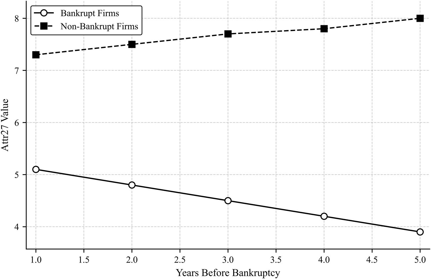
Figure 5 shows the temporal trend of Attr27, which is another crucial measure of stability. The bankrupt firms exhibit a consistent downward trend of Attr27, which decreases from 5.1 in Year 1 to 3.9 in Year 5. Non-bankrupt firms possess a higher but consistent value that increases minimally from 7.3 to 8.0 within the same time. The increasing difference between the two groups emphasizes the role of Attr27 in discriminating financially strong firms from possibly insolvent firms.

Figure 5

Temporal trend of Attr27 over the years for bankrupt and non-bankrupt firms, demonstrating a downward trend in bankrupt firms and stability in non-bankrupt firms (created by the authors).

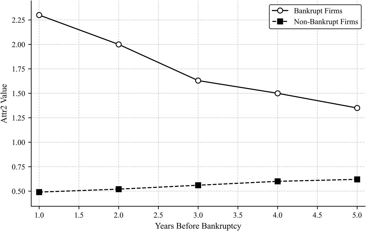
Figure 6 shows the temporal trend of Attr2, which shows a strong positive correlation with bankruptcy. The results indicate that bankrupt firms experience a consistent decline in Attr2, from 2.3 in Year 1 to 1.35 in Year 5. This suggests that as firms approach bankruptcy, their liabilities relative to their assets decrease, likely because of asset liquidation. By contrast, non-bankrupt firms maintain a significantly lower and stable Attr2 value, ranging from 0.49 to 0.62. The clear divergence in trends between the two groups suggests that firms with persistently high Attr2 values are at greater risk of financial distress.

Figure 6

Temporal trend of Attr2 over the years for bankrupt and non-bankrupt firms, highlighting a decline in bankrupt firms while non-bankrupt firms remain stable (created by the authors).

Figure 7 presents the temporal trend of Attr51, another financial indicator positively correlated with bankruptcy. Bankrupt firms exhibit a significant increase in Attr51 over time, increasing from 1.8 in Year 1 to 4.5 in Year 5. By contrast, non-bankrupt firms maintain relatively stable and lower values, ranging from 0.6 to 1.0. The increasing trend in bankrupt firms suggests that, as financial distress worsens, firms may experience rising financial obligations relative to their total assets. This reinforces the role of Attr51 as a crucial early warning sign for impending bankruptcy.

Figure 7

Temporal trend of Attr51 over the years for bankrupt and non-bankrupt firms, showing a sharp increase in bankrupt firms while non-bankrupt firms remain stable (created by the authors).

The results of the temporal trend analysis confirm that certain financial indicators are reliable predictors of bankruptcy risk. Negatively correlated features (Attr48 and Attr27) exhibit declining trends in bankrupt firms, whereas financially stable firms maintain consistently high values. Conversely, positively correlated features (Attr2 and Attr51) show increasing trends for bankrupt firms, indicating worsening financial distress. These findings reinforce the predictive value of selected financial indicators and highlight their significance in early bankruptcy detection.

The feature selection process was conducted using PCA to reduce dimensionality while preserving most of the variance in the dataset. PCA is applied to transform the original financial features into a smaller set of uncorrelated principal components that retain essential information for bankruptcy prediction.

Analysis of the top principal components revealed that financially meaningful attributes heavily influenced them. For instance, the components with the highest explained variance are most strongly associated with variables representing leverage ratios, liquidity measures, and profitability indicators. These features are well known in the financial literature to be predictive of bankruptcy, which reinforces the relevance and interpretability of PCA-selected features. This alignment with domain knowledge enhances the transparency of the feature-selection process and ensures that critical financial signals are retained in the reduced input space.

The cumulative explained variance plot presented in Figure 8 illustrates how the cumulative sum of explained variance increases with the number of principal components. The analysis showed that the first 26 principal components were sufficient to retain 95.63% of the total variance in the dataset. This threshold ensures that minimal information is lost, while significantly reducing the number of features compared to the original dataset. The red dashed line in the figure represents the 95% variance threshold, confirming that additional components contribute negligibly to the variance retention.

Figure 8 presents the explained variance per principal component, highlighting the proportion of the variance captured by each principal component. The first few components explained a substantial portion of the variance, with PC1 capturing approximately 17% and PC2 capturing around 15%. The variance explained by the subsequent components decreases sharply, indicating diminishing returns on information retention. The “elbow effect” observed in this figure suggests that most of the relevant financial information is concentrated in the first few components.

Figure 8

Cumulative explained variance versus number of components. The red dashed line represents the 95% variance threshold (created by the authors).

These findings demonstrate that PCA effectively reduces the dimensionality of a dataset while preserving most of the financial information relevant to bankruptcy predictions. The selection of 26 principal components ensures a balance between computational efficiency and predictive power, and optimizes the feature space for further modeling (Figure 9).

Figure 9

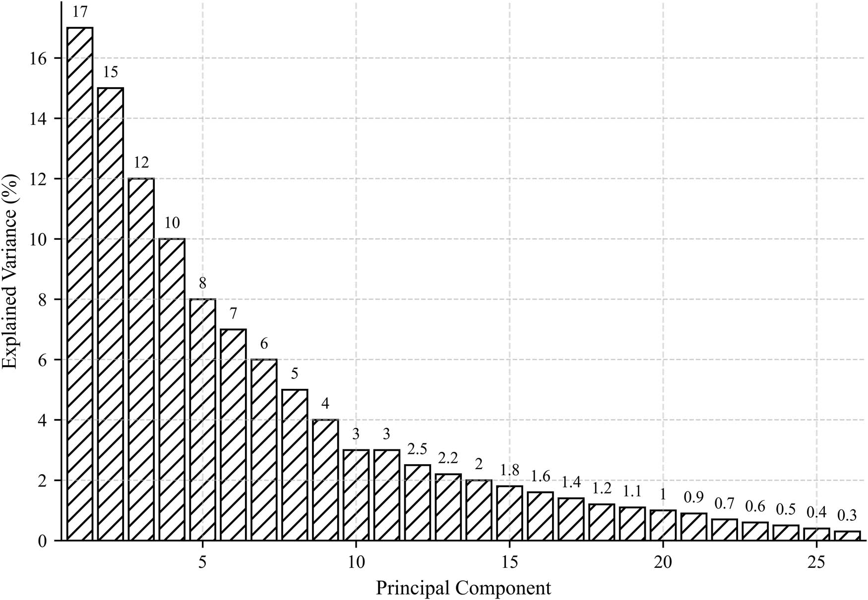
Explained variance per principal component, showing the diminishing returns of additional components (created by the authors).

After applying the PCA, the dataset was transformed into a reduced set of 26 principal components, capturing 95.63% of the total variance. Principal components are linear combinations of the original financial features, with certain attributes contributing more significantly to the retained components. By analyzing the feature loadings, the top financial attributes that contributed the most to the selected principal components were identified. The most influential financial indicators include X2 (total liabilities/total assets), X5 (book value of equity/total liabilities), X7 (EBIT/total assets), X9 (sales/total assets), and X19 (current assets–inventories/short-term liabilities), among others. Such preserved characteristics are crucial finance measures such as leverage, liquidity, profitability, and operational efficiency, which are crucial for discriminating between bankrupt and non-bankrupt firms. The employment of such characteristics means that the best information variables are preserved to avoid redundancy while maintaining predictive capability.

Table 4 presents the average performance measures of the models considered in the 3-year analysis. The models were quantified based on four crucial performance measures: precision, recall, accuracy, and the F-score. The results confirm the efficiency of the proposed HSA-LSTM model in forecasting financial distress.

Table 4

Average performance metrics of the evaluated classification models

Methods	Precision	Recall	Accuracy	F-score
HSA-LSTM	89.46	90.22	90.80	90.54
FLNN	83.58	85.51	87.70	87.20
KELM	79.85	76.28	82.66	80.57
ELM	76.37	77.62	77.96	77.04
SVM	69.05	69.08	69.61	69.48

The HSA-LSTM model achieved the highest overall performance with an average precision of 89.46%, recall of 90.22%, accuracy of 90.80%, and F-score of 90.54%. The results indicated that the model was consistently superior to baseline classifiers in classifying financial distress. The best model was the FLNN model, which was highly predictive, with an accuracy of 87.70% and an F-score of 87.20% but was lower than that of HSA-LSTM.

Among the other models, KELM was moderately predictive with an accuracy rate of 82.66%, whereas ELM and SVM had considerably lower performance with accuracies of 77.96 and 69.61%, respectively. Most noteworthy was that SVM performed the lowest among all the measures, highlighting how unsuitable it was to be used for this bankruptcy prediction problem within this dataset.

The superior performance of the HSA-LSTM can be attributed to its capability to capture temporal relationships within financial data through the LSTM architecture. The use of the HSA to optimize the hyperparameter is also likely to play a role in the enhanced predictive capability. The findings indicate the possibility of using deep learning techniques, specifically optimized RNNs to further improve the models used to predict bankruptcy.

These findings affirm the role of sophisticated machine-learning methodologies in the forecasting of financial distress and indicate that the use of temporal dependencies and hyperparameter optimization can considerably improve model performance.

To further validate the statistical difference in the performance of the models, a one-way ANOVA test was conducted to determine whether there were statistically significant variations among the classification models under consideration. The results show a highly significant difference (F = 114.47, p < 0.0001) among the models, signifying that at least one model performs significantly differently from the remaining models. This confirms that the difference in the classification performance is due to factors other than simply random chance, but rather from the natural variations in the predictive performances of the models.

Following the highly significant ANOVA test statistic, Tukey’s HSD post-hoc test was employed to find specific pairs that were statistically significantly different in performance. The findings shown in Table 2 indicate that the HSA-LSTM model possesses a superior performance to that of the ELM, FLNN, and SVM models, with p-values less than 0.05, providing strong statistical evidence of superior predictive performance. The difference between the FLNN and the HSA-LSTM was highly significant, having an average gain in performance over the latter by 4.26. This implies that, despite the fact that the FLNN classifier is a strong baseline classifier, it is inferior to the proposed method based on deep learning.

However, the difference between KELM and ELM was not statistically significant, as indicated by the p-value of 0.162. This indicates that the two models performed at a comparable rate, providing similar predictive precision. Meanwhile, the difference between the performances of the two models was statistically significant, where the mean performance was significantly lower for the SVM, which indicates the inefficiency of the latter in forecasting financial distress. Table 5 shows the results of the comparison of performances using Tukey’s HSD test.

Table 5

Tukey’s HSD test results comparing model performance

Model 1	Model 2	Mean difference	p-value	Lower bound	Upper bound	Significant difference
ELM	FLNN	8.75	0.000	5.45	12.05	Yes
ELM	HSA-LSTM	13.01	0.000	9.71	16.31	Yes
ELM	KELM	2.59	0.162	−0.71	5.89	No
ELM	SVM	−7.94	0.000	−11.24	−4.64	Yes
FLNN	HSA-LSTM	4.26	0.009	0.96	7.56	Yes

These statistical results have strong practical implications for bankruptcy prediction. The HSA-LSTM model demonstrated the highest performance, with a mean improvement of 13.01 over ELM (p = 0.000) and 4.26 over FLNN (p = 0.009), indicating a consistent and measurable advantage in prediction accuracy. In contrast, SVM underperformed significantly, showing a 7.94 point deficit compared with ELM (p = 0.000), confirming its limited suitability for this task. The non-significant difference between KELM and ELM (p = 0.162) suggests that these models offer similar predictive precision. Overall, these findings quantitatively validate HSA-LSTM’s superior predictive reliability and its value for deployment in financial risk systems.

6 Discussion

The findings of this study validate the effectiveness of the proposed HSA-LSTM model for company bankruptcy prediction, with superior accuracy over traditional and machine learning-based classifiers. The integration of LSTM networks with the HSA for hyperparameter tuning is accountable for the superior classification accuracy on diverse evaluation measures. The HSA-LSTM produced an accuracy of 90.80%, precision of 89.46%, recall of 90.22%, and F-score of 90.54%, indicating its financial distress prediction capability. Compared with benchmarking models such as FLNN, KELM, ELM, and SVM, the proposed model consistently produced superior performance across various forecasting horizons, thereby validating its temporal relationship identification capability in financial data.

One of the key strengths of the HSA-LSTM model is that it can process sequential financial data more effectively, thereby addressing the shortcomings of traditional machine-learning models that rely on static features. The LSTM network can store previous information using its memory cells, which allows it to recognize long-term financial trends linked to the risk of bankruptcy. In addition, the HSA contributed significantly to model hyperparameter optimization, thereby limiting the requirement for manual tuning and enhancing classification efficacy. The experimental results reveal that hyperparameter optimization has a significant influence on predictive performance because models lacking HSA tuning performed worse.

The statistical tests also corroborated the significance of the results. The use of a one-way ANOVA test validated that the model performance differences were statistically significant (p < 0.0001), indicating that the gains observed in the proposed model did not occur by chance. Moreover, Tukey’s HSD post-hoc test revealed statistically significant differences between the HSA-LSTM model and baseline classifiers (FLNN, ELM, and SVM), thereby validating the efficacy of the proposed method. Interestingly, the SVM model performed the worst with 69.61% accuracy, reflecting its lack of capability in handling complicated financial data. In comparison, KELM and ELM achieved decent classification performance, indicating that kernel-based methods and single-hidden-layer neural networks still provide competitive performance but lack the sequential processing advantage of LSTM networks.

In practical settings, the proposed HSA-LSTM model can be integrated into the early warning systems used by banks and regulatory bodies. Financial institutions can deploy the model as part of credit risk-scoring systems by feeding them periodic financial reports. Integration involves establishing a pipeline for data ingestion, preprocessing, prediction, and explainability analysis, followed by a human-in-the-loop review for critical decisions. Regulatory compliance, data privacy, and system scalability must also be addressed during deployment.

Despite its strong performance, the HSA-LSTM model has limitations. The imbalanced nature of the dataset, which has a lesser representation of bankrupt entities compared with the total data, can still result in biased predictions by the model. Although LSTM networks have better sequence learning abilities, their computational requirements are higher than those of traditional classifiers, making them resource-intensive when dealing with large financial datasets. Additionally, while PCA has been utilized to reduce data dimensionally, other feature selection methods, such as autoencoders or mutual information-based approaches, may be used in future research to continue enhancing model interpretability and effectiveness.

Practically, this study underscores the potential of sophisticated machine learning and optimization algorithms to predict financial distress. The HSA-LSTM tool is an effective computational and scalable early warning system that can be employed by investors, financial institutions, and policymakers to evaluate risks and make decisions. The ability to predict bankruptcy years in the future can allow early intervention measures that can curb financial losses and strengthen corporate governance to be taken. The key limitations of this study are as follows.

The dataset is skewed toward non-bankrupt companies, which can bias model predictions and reduce the sensitivity to minority classes.
LSTM-based models require a longer training time and computational resources, particularly with large-scale financial data.
Deep learning architecture lacks transparency, which may limit its adoption in regulatory or decision-critical environments.
Although PCA has been applied, more sophisticated or nonlinear feature selection methods may yield improved results.
The findings are based solely on Polish companies, and their generalizability to other economic contexts remains untested.
Future research can take other directions to enhance the predictive capability of deep-learning models. First, the use of macroeconomic indicators, industry finance trends, and other forms of alternative data (such as sentiment analysis from news and social media analysis) can add more depth to the model inputs and enhance the predictive capability. Second, the integration of XAI techniques can make the models more interpretable to deliver more information about the most important finance indicators connected to the risk of bankruptcy. Third, the use of cost-sensitive learning or synthetic data creation algorithms can alleviate the problem of class imbalance and deliver more accurate classification results for minority classes ( bankrupt classes). Fourth, a critical extension would be to incorporate explainability techniques, such as SHAP or LIME, to identify which financial variables most influence predictions. This enhances model transparency, an essential requirement for adoption by financial institutions and regulators. Finally, in the present study, we did not apply explicit resampling methods, such as SMOTE or ADASYN. Instead, the model’s architecture and evaluation metrics were designed to maintain the sensitivity to minority classes. However, integrating such techniques into future versions of the model could further improve the performance of underrepresented cases.

7 Conclusion

This study presents a hybrid deep learning approach to forecasting corporate bankruptcy that combines the use of LSTM networks with the HSA to tune the hyperparameters. Using a real-world database of Polish companies made available by the EMIS, the study indicated that the use of PCA to undertake feature selection was successful in reducing dimensionality and maintaining forecasting capability.

The proposed HSA-LSTM model significantly outperformed the baseline classifiers, with 90.80% accuracy, 89.46% precision, 90.22% recall, and an F-score of 90.54%. The suggested model consistently exhibited a higher performance than FLNN, KELM, ELM, and SVM under different forecasting periods. The improvements were statistically confirmed using ANOVA and Tukey’s HSD test (p < 0.05), validating the forecasting capability of the model.

This research provides an added contribution to early bankruptcy identification and finance risk management via an efficient and scalable framework based on deep learning that assists corporate decision-making. Future work can explore other metaheuristic optimization algorithms, explainable AI models, and macroeconomic indicators to further improve predictive performance and understandability.

Overall, this study verifies the effectiveness of LSTM models employed to forecast financial distress if accompanied by hyperparameter optimization and feature selection. This study provides valuable information to investors, analysts, and policymakers making projections within the finance sector.

Funding information: The authors received no financial support for the research, authorship, or publication of this article.
Author contributions: Mohamed Elhoseny conceptualized the research idea and led the design of the methodology. Mohamed Elhoseny and Mohanad A. Deif developed the software implementation, performed the primary data analysis, and drafted the initial manuscript. Saadat M. Alhashmi contributed to the development and optimization of the HSA-LSTM model and supported the experimental evaluations. Noura Metawa and Rhada Boujlil coordinated data acquisition and preparation, and contributed to the statistical analysis and definition of performance metrics. All authors participated in the literature review, interpretation of results, critical revision of the manuscript, and preparation of visual materials. All authors have read and approved the final version of the manuscript.
Conflict of interest: The authors declare that there is no conflict of interest regarding the publication of this manuscript.
Data availability statement: The dataset used in this study is publicly available from the UCI Machine Learning Repository under the title Polish companies bankruptcy data, compiled by Tomczak [31].

References

[1] Shetty S, Musa M, Brédart X. Bankruptcy prediction using machine learning techniques. J Risk Financial Manag. 2022;15(1):35. 10.3390/jrfm15010035.Suche in Google Scholar

[2] Tabbakh A, Rout JK, Sahoo KS, Jhanjhi NZ, Shah MH, Rout M. Bankruptcy prediction using robust machine learning model. Turk J Comput Math Educ. 2021;12(10):3060–73.Suche in Google Scholar

[3] Sulistiani I, Mufida E, Yasser PM, Alamsyah L. Systematic literature review: Bankruptcy prediction menggunakan teknik machine learning dan deep learning. INTECH (Inf Teknol). 2021;2(1):13–8. 10.54895/intech.v2i1.824.Suche in Google Scholar

[4] Sufi A, Taylor AM. Financial crises: A survey. Handb Int Econ. 2022;6:291–340. 10.1016/bs.hesint.2022.02.012.Suche in Google Scholar

[5] Laborda R, Olmo J. Volatility spillover between economic sectors in financial crisis prediction: Evidence spanning the great financial crisis and Covid-19 pandemic. Res Int Bus Financ. 2021;57:101402. 10.1016/j.ribaf.2021.101402.Suche in Google Scholar

[6] Greenacre M, Groenen PJF, Hastie T, d’Enza AI, Markos A, Tuzhilina E. Principal component analysis. Nat Rev Methods Primers. 2022;2(1):100. 10.1038/s43586-022-00184-w.Suche in Google Scholar

[7] Hasan BMS, Abdulazeez AM. A review of principal component analysis algorithm for dimensionality reduction. J Soft Comput Data Min. 2021;2(1):20–30. 10.30880/jscdm.2021.02.01.003.Suche in Google Scholar

[8] Elhoseny M, Metawa N, Sztano G, El-Hasnony IM. Deep learning-based model for financial distress prediction. Ann Oper Res. 2025;345:885–907. 10.1007/s10479-022-04766-5.Suche in Google Scholar PubMed PubMed Central

[9] Ahmed FR, Alsenany SA, Abdelaliem SMF, Deif MA. Development of a hybrid LSTM with chimp optimization algorithm for the pressure ventilator prediction. Sci Rep. 2023;13(1):20927. 10.1038/s41598-023-47837-8.Suche in Google Scholar PubMed PubMed Central

[10] Nancy M, Stephen SEA. A comprehensive review on harmony search algorithm. Ann Rom Soc Cell Biol. 2021;25(5):5480–3. 10.3390/ijfs11010038.Suche in Google Scholar

[11] Pang S, Du L. Deep learning: a study on financial crisis forewarning in small and medium-sized listed enterprises. J Control Decis. 2024;24(3):1–15. 10.1080/23307706.2024.2331546.Suche in Google Scholar

[12] Zhao Y. Design of a corporate financial crisis prediction model based on improved ABC-RNN+Bi-LSTM algorithm in the context of sustainable development. PeerJ. 2023;15(2):45–60. 10.7717/peerj-cs.1287.Suche in Google Scholar PubMed PubMed Central

[13] Tang D. Optimization of financial market forecasting model based on machine learning algorithm. Proc Bus Econ Stud. 2023;27(1):85–98. 10.1109/ICNETIC59568.2023.00104.Suche in Google Scholar

[14] Li S, Chen X. An effective financial crisis early warning model based on an IFOA-BP neural network. J Internet Technol. 2024;25(5):100–15. 10.53106/160792642024052503009.Suche in Google Scholar

[15] Guo R. Financial crisis prediction based on genetic algorithm and LS-SVM. J Comput Financ. 2022;28(3):132–49. 10.1109/ICAICA54878.2022.9844522.Suche in Google Scholar

[16] Kalaivani S. Chimp optimization algorithm-based kernel extreme learning machine for financial risk forecasting. Neural Comput Appl. 2023;35(2):3401–15. 10.3934/NAR.2021012.Suche in Google Scholar

[17] Abdul-kareem AA, Fayed ZT, Rady S, El-Regaily SA, Nema BM. An intelligent decision support system for forecasting financially distressed businesses. Proc AI Financ. 2023;10(4):50–65. 10.1109/ICICIS58388.2023.10391150.Suche in Google Scholar

[18] Purnell Jr D, Etemadi A, Kamp J. Developing an early warning system for financial networks: an explainable machine learning approach. Entropy. 2024;26(5):66–79. 10.3390/e26090796.Suche in Google Scholar PubMed PubMed Central

[19] Jian K, Yu S. Financial Crisis Prediction Based on GWO-SVM. In 2023 2nd International Conference on Artificial Intelligence, Internet and Digital Economy (ICAID 2023). Atlantis Press; 2023. p. 535–43. 10.2991/978-94-6463-222-4_58.Suche in Google Scholar

[20] Quan C, Yuan YH, Wang G, Wu HT. Optimization of enterprise financial risk management and crisis early warning system supported by AI. J Glob Inf Manag. 2024;32(5):200–20. 10.4018/JGIM.356490.Suche in Google Scholar

[21] Torky M, et al. Enhancing financial crisis prediction with explainable AI models using pigeon optimization algorithm. Appl Soft Comput. 2023;135:85–97. 10.1007/s44196-023-00222-9.Suche in Google Scholar

[22] Chen Y, Andrew X, Supasanya S. CRISIS ALERT: Forecasting stock market crisis events using machine learning methods. arXiv preprint arXiv:2401.06172; 2024. 10.48550/arXiv.2401.06172.Suche in Google Scholar

[23] Tan B, Gan Z, Wu Y. The measurement and early warning of daily financial stability index based on XGBoost and SHAP: Evidence from China. Expert Syst Appl. 2023;227. 10.1016/j.eswa.2023.120375.Suche in Google Scholar

[24] Zhang Z, Liu X, Niu H. Financial crisis early warning of Chinese listed companies based on MD&A text-linguistic feature indicators. Plos One. 2023;18(9):e0291818.10.1371/journal.pone.0291818Suche in Google Scholar PubMed PubMed Central

[25] Qiang T. Supervised learning-based financial crisis forecasting for emerging economies. Afr J Financ Bank Stud. 2024;11(1):88–104. 10.1145/3501305.Suche in Google Scholar

[26] Wang J, Lu S, Wang S-H, Zhang Y-D. A review on extreme learning machine. Multimed Tools Appl. 2022;81(29):41611–60. 10.1007/s11042-021-11007-7.Suche in Google Scholar

[27] Ju C, Zhu Y. Reinforcement learning‐based model for enterprise financial asset risk assessment and intelligent decision‐making; Appl Comput Eng. 2024;97:181–6. 10.20944/preprints202410.0698.v1.Suche in Google Scholar

[28] Li F, Chen Y, Sun J. Transfer learning in bankruptcy prediction: adapting pre-trained models for financial risk forecasting. Int J Mach Learn Appl. 2024;17(2):89–103.Suche in Google Scholar

[29] Feng X, et al. Stacking ensemble learning for bankruptcy prediction: an empirical study. IEEE Trans Comput Intell Financ. 2024;12(2):198–215.Suche in Google Scholar

[30] Zhao M. Bayesian neural networks for financial risk assessment: a probabilistic deep learning approach. J Risk Financ Stab. 2024;36(1):28–41.Suche in Google Scholar

[31] Tomczak S. Polish companies bankruptcy data. UCI Machine Learning Repository; 2016. 10.24432/C5F600.Suche in Google Scholar

[32] Faul F, Erdfelder E, Buchner A, Lang A-G. Statistical power analyses using G* Power 3.1: Tests for correlation and regression analyses. Behav Res Methods. 2009;41(4):1149–60. 10.3758/BRM.41.4.1149.Suche in Google Scholar PubMed

[33] Kurita T. Principal component analysis (PCA). In Computer vision: a reference guide. Cham, Switzerland: Springer; 2021. p. 1013–6. 10.1007/978-3-030-63416-2_649.Suche in Google Scholar

[34] Zheng S, Ristovski K, Farahat A, Gupta C. Long short-term memory network for remaining useful life estimation. In 2017 IEEE International Conference on Prognostics and Health Management (ICPHM). 2017. p. 88–95. 10.1109/ICPHM.2017.7998311.Suche in Google Scholar

[35] Liu Y, Li D, Wan S, Wang F, Dou W, Xu X, et al. A long short-term memory-based model for greenhouse climate prediction. Int J Intell Syst. 2022;37(1):135–51. 10.1002/int.22620.Suche in Google Scholar

[36] Gupta S. Enhanced harmony search algorithm with non-linear control parameters for global optimization and engineering design problems. Eng Comput. 2022;38(Suppl 4):3539–62. 10.1007/s00366-021-01467-8.Suche in Google Scholar

[37] Jayalakshmi P, Sridevi S, Janakiraman S. A hybrid artificial bee colony and harmony search algorithm-based metahueristic approach for efficient routing in WSNs. Wirel Pers Commun. 2021;121(4):3263–79. 10.1007/s11277-021-08875-5.Suche in Google Scholar

[38] Luo N, Yu H, You Z, Li Y, Zhou T, Jiao Y, et al. Fuzzy logic and neural network-based risk assessment model for import and export enterprises: A review. J Data Sci Intell Syst. 2023;1(1):2–11. 10.47852/bonviewJDSIS32021078.Suche in Google Scholar

[39] Murmu S, Biswas S. Application of fuzzy logic and neural network in crop classification: a review. Aquat Procedia. 2015;4:1203–10. 10.1016/j.aqpro.2015.02.153.Suche in Google Scholar

[40] Luo F, Liu G, Guo W, Chen G, Xiong N. ML-KELM: A kernel extreme learning machine scheme for multi-label classification of real time data stream in SIoT. IEEE Trans Netw Sci Eng. 2021;9(3):1044–55. 10.1109/TNSE.2021.3073431.Suche in Google Scholar

[41] Xie G, Attar H, Alrosan A, Abdelaliem SMF, Alabdullah AAS, Deif M. Enhanced diagnosing patients suspected of sarcoidosis using a hybrid support vector regression model with bald eagle and chimp optimizers. PeerJ Comput Sci. 2024;10:e2455. 10.7717/peerj-cs.2455.Suche in Google Scholar PubMed PubMed Central

[42] Choi Y, Park S, Park C, Kim D, Kim Y. META-ANOVA: Screening interactions for interpretable machine learning. arXiv preprint arXiv:2408.00973. 2024. 10.48550/arXiv.2408.00973.Suche in Google Scholar

[43] Abdi H, Williams LJ. Tukey’s honestly significant difference (HSD) test. Encycl Res Des. 2010;3(1):1–5.Suche in Google Scholar

[44] Nanda A, Mohapatra BB, Mahapatra APK, Mahapatra APK, Mahapatra APK. Multiple comparison test by Tukey’s honestly significant difference (HSD): Do the confident level control type I error. Int J Stat Appl Math. 2021;6(1):59–65. 10.22271/maths.2021.v6.i1a.636.Suche in Google Scholar

Received: 2025-03-12

Accepted: 2025-06-27

Published Online: 2025-09-05

This work is licensed under the Creative Commons Attribution 4.0 International License.

Artikel in diesem Heft

https://doi.org/10.1515/jisys-2025-0058

Schlagwörter für diesen Artikel

deep learning; artificial intelligence; bankruptcy prediction; financial risk management; metaheuristic optimization

Creative Commons

BY 4.0