Hybridizing the Cuckoo Search Algorithm with Different Mutation Operators for Numerical Optimization Problems
-
Bilal H. Abed-alguni
 and
David J. Paul
and
David J. Paul

Abstract
The Cuckoo search (CS) algorithm is an efficient evolutionary algorithm inspired by the nesting and parasitic reproduction behaviors of some cuckoo species. Mutation is an operator used in evolutionary algorithms to maintain the diversity of the population from one generation to the next. The original CS algorithm uses the Lévy flight method, which is a special mutation operator, for efficient exploration of the search space. The major goal of the current paper is to experimentally evaluate the performance of the CS algorithm after replacing the Lévy flight method in the original CS algorithm with seven different mutation methods. The proposed variations of CS were evaluated using 14 standard benchmark functions in terms of the accuracy and reliability of the obtained results over multiple simulations. The experimental results suggest that the CS with polynomial mutation provides more accurate results and is more reliable than the other CS variations.
1 Introduction
Nature-inspired optimization (NIO) algorithms are a class of optimization algorithms that simulate different natural phenomena to solve NP-hard problems or problems with high complexity. NIO algorithms such as the genetic algorithm (GA) [14], [19], Cuckoo search (CS) [6], harmony search (HS) [25], Bat algorithm (BA) [3], whale optimization algorithm (WOA) [8], [33], ant colony optimization (ACO), particle swarm optimization (PSO) [12], and Krill herd algorithm (KHA) [24] have shown high performance in solving both discrete and continuous optimization problems.
The CS algorithm [42] is an NIO algorithm that simulates the nesting and parasitic reproduction behaviors of some cuckoo species. It starts its evolution process with n candidate solutions (eggs). At each generation of the CS algorithm, a cuckoo’s egg (i.e. a random candidate solution) is selected using a uniformly random function in an attempt to improve it using a mutation-like function based on the Lévy flight operator. The algorithm then replaces an egg of a host bird (i.e. another candidate solution selected randomly) from the population of solutions with the cuckoo’s egg, only if the objective value of the cuckoo’s egg is better than the objective value of the egg of the host bird. Finally, the CS algorithm replaces a portion of the worst eggs with randomly generated eggs.
Many research studies in the literature have shown the efficiency of Lévy flight as a mutation and exploration method for real-world optimization problems [2], [5], [13], [34], [42], [43], [44]. The goal of the current research study is to evaluate the performance of CS after replacing the Lévy flight based update function with different mutation methods adopted from different evolutionary algorithms.
Mutation operators are mainly used to avoid getting trapped in local optima when solving a given optimization problem [26]. Although the mutation concept was first introduced in the GA algorithm, several evolutionary algorithms, such as HS and CS, apply special mutation operators to produce new solutions or alter some features of a candidate solution.
The main purpose of this paper is to investigate the suitability and efficiency of seven mutation methods as replacements for the Lévy flight based update function in CS, namely, random, boundary, non-uniform, MPT (Makinen, Periaux and Toivanen), power, polynomial, and pitch adjustment mutation methods [26], [31]. These mutation methods were modified to be applicable to CS, as described in Section 4. The proposed seven variations of CS were evaluated using a set of 14 popular benchmark functions in terms of the accuracy and reliability of the obtained results over multiple simulations. The obtained results indicate that CS with polynomial mutation provides more accurate and stable results than the other algorithms for a considerable number of the benchmark functions.
The rest of the paper is organized as follows: the CS algorithm is explained in Section 2, the related work to CS is overviewed in Section 3, Section 4 presents the different mutation methods, Section 5 presents the experimental results, and finally, Section 6 presents the conclusion of this paper.
2 CS Algorithm
Inspired by the parasitic breeding behavior of some cuckoo species and the Lévy flight behavior of birds, Yang and Deb [42] formulated and introduced the CS optimization algorithm. The inhabitants of some cuckoo species commonly rely on other birds (host birds) to raise their baby birds. This phenomenon is known as a parasitic reproduction strategy in which a cuckoo bird lays its eggs on a nest of a host bird, taking the risk that the host bird may discover the cuckoo’s eggs. If the host bird discovers the cuckoo’s eggs, it rejects the eggs (discards the eggs or abandons its nest); otherwise, the host bird tends to the cuckoo’s egg as if it were its own. The CS algorithm attempts to solve a wide range of optimization problems based on two simulation models: a model that simulates the parasitic reproduction strategy of some cuckoo species and another model that simulates the Lévy flight behavior of some bird species [16], [35], [42].
According to the terminologies of CS, a candidate solution is called an egg and a new solution is called a cuckoo’s egg. The CS algorithm attempts to generate new solutions (cuckoos’ eggs) using the Lévy flight operator for potential replacement with lower quality solutions in the population (eggs in the nests). The CS algorithm depends mainly on two parameters, the population size n (i.e. the number of candidate solutions) and the fragment of the candidate solutions that are going to be discarded at each iteration of CS (pa ∈ [0, 1]). The following notations and assumptions formulate the mathematical model of the original CS algorithm:
A candidate solution
The value of a decision variable xi is randomly generated using the function
The fitness value of the candidate solution X is f(X).
Th population size is denoted as n, which is a fixed number that represents the number of candidate solutions. An augmented matrix of size n × m is used to represent the population of n candidate solutions:
(1)The CS algorithm replaces a fraction pa ∈ [0, 1] of the population (solutions with the lowest fitness values) with new randomly generated solutions at the last step of each generation of CS.
At the end of each generation of CS, the best candidate solutions are moved to the next generation of CS.
The CS algorithm starts by generating a population of n nominated solutions Xi (i = 1, 2, …, n) from the range of potential solutions of the objective function f(Xi). In addition, the termination condition or the maximum number of iterations (MaxItr) of the algorithm is specified based on the optimal value/s of f(Xi).
The CS algorithm attempts to improve a candidate solution
where β > 0 is the distance parameter that determines the distance of mutation and the symbol ⊕ represents the entry-wise product operator. The Lévy flight is a special random walk in which the step length is a random number generated from a heavy tailed Lévy distribution with a power law:
where D is the step size and α ∈ (1, 3] is a parameter related to fractal dimension (i.e. a ratio that provides a statistical index of complexity and that compares details in a fractal pattern). An interesting property of the Lévy distribution function is that it has infinite variance [42]. This property indicates that some of the generated random solutions will be close to the local optima, while a large percentage of the generated solutions will be random solutions far from the local optima. This means that the Lévy flight is more efficient in exploring the search space than the random walk method because the distance value in the Lévy flight method increases over the course of generations.
3 Related Work
Most research studies that have attempted to improve the performance of CS have focused on hybridizing the CS algorithms with other search techniques or evolutionary operators. Kanagaraj et al. [28] incorporated the evolutionary operators (crossover and mutation) of the GA into CS. The new algorithm, which is called the hybrid CS and GA (HCSGA) algorithm, is used to provide solutions for constrained engineering design optimization problems. The crossover and mutation operators are used at each iteration of CS to balance the ratio of exploration and exploitation. According to the simulation results in ref. [28], HCSGA provides good performance compared to CS, PSO, and Global convergence PSO (GCPSO). Kanagaraj et al. [27] designed another hybrid CS and GA algorithm (CS-GA) to solve the reliability-redundancy allocation problem (RAP). RAP is an optimization problem that involves finding an optimal allocation plan for redundant subsystems subject to a set of predefined resource constraints. The simulation results in ref. [27] suggest that CS-GA provides a competitive performance compared to popular optimization algorithms [e.g. CS, artificial bee colony (ABC) [38], HS]. Saraswathi et al. [36] introduced a hybrid CS and BA algorithm. The hybrid CS and BA algorithm was designed to find an optimal path in the mobile robot path planning problem. Wang et al. [41] introduced a new hybrid CS algorithm called CS/HS, which incorporates the pitch adjustment operator of the HS algorithm into the CS algorithm to speed up the convergence speed of CS. The simulation results in ref. [41] suggested that CS/HS outperforms many standard optimization algorithms. Wang et al. [40] introduced a hybrid optimization algorithm called CSKH, which uses the update rule and abandon method of CS inside the improvement loop of KHA. In another related work, Wang et al. [39] proposed the Lévy flight Krill herd (LKH) algorithm, which incorporates the Lévy flight operator into the KHA algorithm to improve its global search ability. LKH was experimentally proven to be an efficient algorithm, according to ref. [39]. However, CSKH and LKH have complex structures and require more computations compared with KHA and CS. It is important to note that, in general, the hybrid CS algorithms have complex structures and require more computational time than standard optimization algorithms do (e.g. CS, GA, ABC, HS, BA, KHA).
The established efficiency and usability of the mutation methods in the GA algorithm have encouraged many researchers to adopt the use of several mutation methods with evolutionary algorithms such as the HS and CS algorithms. These algorithms apply special mutation operators to produce new solutions or alter some features of a candidate solution. The random, boundary, non-uniform, MPT, power, polynomial, and pitch adjustment mutation methods were used to enhance the performance of the ABC algorithm [22]. The same mutation methods were also used to improve the efficiency of the HS algorithm [26].
4 Mutation Operators
The original CS algorithm applies the Lévy flight method to explore the search space. This method alters the values of the decision variables of a candidate solution based on equation (2). This paper introduces seven variations of the CS algorithm using different mutation methods. Each one of the proposed variations replaces the Lévy flight method with a unique mutation method.
Several mutation operators can be used with the evolutionary algorithms based on the representation of the optimization problems. In this section, the mutation operators that are suitable for continuous optimization problems will be presented. These mutation operators have been used with the GA [31], HS [26], and ABC [22] algorithms. The experimental results in refs. [22], [26] indicate that most of the mutated optimization algorithms perform better than the original algorithms do. The efficiency of a mutation operator is normally affected by the type of the optimization problem and the strength of the population (i.e. how far is the mutated solution from the initial population) [26].
4.1 Random Mutation
The random mutation method is a basic mutation method that is usually used in GAs [26], [31]. In this method, the value of a gene (decision variable) of a chromosome (candidate solution) is replaced with a randomly generated value from the range of possible solutions of the gene as follows:
where U(0, 1) is a uniform random number between 0 and 1.
The authors in refs. [5], [42] suggested that the Lévy flight method is more efficient in exploring the search space than the random mutation method. However, the random mutation method was not used in refs. [5], [42] as a mutation method for the CS. It was actually used as a mutation method for the GA algorithm. Therefore, it would be interesting to evaluate the performance of CS after replacing the Lévy flight method with the random mutation method.
4.2 Boundary Mutation
The boundary mutation method is a mutation method that is traditionally used with evolutionary algorithms for integer or floating point decision variables [26], [31]. A new solution can be generated using this method by randomly replacing the value of a decision variable of a candidate solution with its lower or upper bound (
4.3 Non-Uniform Random Mutation
The non-uniform random mutation is a well-known mutation method that is commonly used in GAs to overcome the disadvantages of random mutation [26], [31], [32]. The probability that the amount of mutation will approach zero by the end of the evolution process increases with the non-uniform random mutation method. It helps the population of solutions evolve in the early stages of the evolution process, which helps to avoid local optima. It also helps in increasing the accuracy of the solutions by finely tuning the solutions at the final stages of the evolution process.
Given a candidate solution
where LBi is the lower bound and UBi is the upper bound of xk.
The value returned from Δ(t, y) is in the range [0, y] such that the probability of Δ(t, y) approaches zero with each increase in the number of generations t. This property means that the search process will be uniform when t is small (early generations) but will get closer to local values over the course of iterations. The following function has been used in the experimental section of the paper to calculate Δ(t, y):
where U(0, 1) is a random number between 0 and 1, maxt is the maximum number of generations, and b is a parameter that determines the degree of dependency on the generation number (b was set to 1 and 5 in the experimental section, as suggested in ref. [32]). The above function aims to increase the probability of producing new values near the previously produced values instead of generating random values [26], [31], [32].
4.4 MPT Mutation
MPT mutation was proposed by Makinen et al. [37]. It is a mutation method that has been used to solve several types of optimization problems such as the multidisciplinary shape optimization problems and optimization problems with a constrained nature [22]. A decision variable xi can be mutated using MPT to generate a new variable
uniformly generate a random number ri ∈ [0, 1]
and
where LBi is the lower bound and UBi is the upper bound of xi. It is worth pointing out that the efficiency of the MPT mutation method is not affected by the generation number, unlike the non-uniform random mutation method. In the experimental section, the value of b for the MPT method was set to 1 and 5, as suggested in ref. [37].
4.5 Power Mutation (PM)
Deep and Thankur [20] introduced the PM method, which is based on power distributions. The function of the power distribution is represented as follows:
and the density function is as follows:
where p represents the index of the distribution.
Given a decision variable x, the PM method generates a new solution x′ according to the following steps:
Generate a new random number r between 0 and 1.
Create a random number s based on the final distribution.
Calculate t as follows:
(11)where LB is the lower bound and UB is the upper bound of x.
Create a new solution x′ as follows:
(12)
In the experimental section, the value of b for the PM method was set to 0.25 and 0.5, as suggested by Deep and Thankur in ref. [20].
4.6 Highly Disruptive Polynomial (HDP) Mutation
The polynomial mutation method suggested by Deb and Agrawal in ref. [17] may get trapped in a local optima when the value of a decision variable that is to be mutated is near one of its boundaries. HDP mutation [18] is an enhanced variation of the polynomial mutation. The value of a decision variable xi can be mutated using the HDP method, as described in the algorithm in Figure 1. In Figure 1, r is a random number between 0 and 1, Pm is the probability of mutation, LBi is the lower boundary of xi, UBi is the upper boundary of xi, δ1 is the difference between xi and LBi divided by UBi − LBi, δ2 is the difference between UBi and xi divided by UBi − LBi, and ηm is a non-negative number that represents the distribution index. An advantage of the HDP method over the polynomial method is that it can sample the whole search space of the decision variable even if the variable’s value is near to one of its boundaries.

Highly Disruptive Polynomial Mutation.
4.7 Pitch Adjustment
The pitch adjustment method is a special mutation method used in the HS algorithm [25], [29]. Given a vector of m decision variables (a candidate solution)
If PAR is greater than or equal to a randomly generated number (r ∈ [0, 1]), the value of
4.8 Worst Case Analysis of Computational Complexity of Mutation Operators
The purpose of this section is to discuss the computational complexity of each mutation operator discussed in Section 4 for a single iteration of CS. In the following analysis, it is assumed that a mutation operator is applied to all decision variables. However, in practice, it is applied to one or only a few decision variables.
Assume a candidate solution with m decision variables
| Abbreviation | Function name | Search range | D | |
|---|---|---|---|---|
| f1 | De Jong’s first function | [−100, 100] | m | 0 |
| f2 | Schwefel 2.22 function | [−100, 100] | m | 0 |
| f3 | Step function | [−100, 100] | m | 0 |
| f4 | Rosenbrock’s function | [−2.048, 2.048] | m | 0 |
| f5 | Rotated hyper-ellipsoid function | [−100, 100] | m | 0 |
| f6 | Schwefel 2.26 function | [−500, 500] | m | −12569.5 |
| f7 | Rastrigin’s function | [−5.12, 5.12] | m | −1 |
| f8 | Ackley’s function | [−32.77, 32.77] | m | 0 |
| f9 | Griewank’s function | [−600, 600] | m | 0 |
| f10 | Six-hump camel-back | [−5, 5] | 2 | −1.031628 |
| f11 | Shifted sphere function | [−100, 100] | m | −450 |
| f12 | Shifted Schwefel’s problem 1.2 | [−100, 100] | m | −450 |
| f13 | Shifted Rosenbrock’s function | [−100, 100] | m | 390 |
| f14 | Shifted Rastrigin’s function | [−5, 5] | m | −330 |
4.9 CS with Mutation
This section shows how the Lévy flight method in the original CS algorithm can be replaced with one of the seven different mutation methods discussed in Section 4.
Simple modifications should be conducted to incorporate one of the seven mutation operators into CS, as shown in Figure 2 (lines 4 and 6). In line 4, one of the mutation operators discussed in Section 4 should be selected before the beginning of the improvement loop of CS (lines 5–16). In line 6, the algorithm attempts to improve a candidate solution (
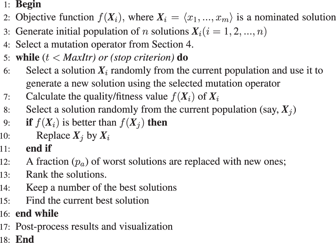
CS with Mutation.
Different Variations of CS.
| Abbreviation | Variation of CS |
|---|---|
| CS1 | CS with Lévy flight with D = 1 |
| CS2 | CS with random mutation |
| CS3 | CS with boundary mutation |
| CS4 | CS with non-uniform random mutation with b = 1 |
| CS5 | CS with non-uniform random mutation with b = 5 |
| CS6 | CS with MPT mutation with b = 1 |
| CS7 | CS with MPT mutation with b = 5 |
| CS8 | CS with power mutation with b = 0.25 |
| CS9 | CS with power mutation with b = 0.5 |
| CS10 | CS with HDP mutation |
| CS11 | CS with pitch adjustment mutation with PAR =0.3 |
5 Experiments
5.1 Benchmark Functions
In this section, 11 variations of CS (see Table 2) were compared and evaluated using 14 benchmark functions (see Table 1). This set of benchmark functions has been used in the literature to evaluate evolutionary algorithms with mutation methods [22], [26]. The threshold values in CS4 and CS5, CS6 and CS7, CS8 and CS9 were used in refs. [20], [22], [26] to evaluate mutated variations of the HS and ABC algorithms.
5.2 Setup
The experiments were conducted using an Intel Core i5 6th Gen CPU (3.4 GHz) with 8-GB RAM running macOS 10.13, High Sierra (Cupertino, CA, USA). All of the algorithms were implemented using the Java programming language.
All the CS variations used the same parameter settings: n = 10, pa = 0.25, and the mutation rate r = 0.05. These values are based on those used in refs. [2], [5], [13], [42], [43].
Simulation Results of the CS Variations for 14 Standard Test Functions, Number of Decision Variables = 30, Number of Runs = 50, and Maximum Number of Iterations = 10,000.
| Function | CS1 | CS2 | CS3 | CS4 | CS5 | CS6 | CS7 | CS8 | CS9 | CS10 | CS11 |
|---|---|---|---|---|---|---|---|---|---|---|---|
| F1 | 5.13E−06 | 3.71E−07 | 2.62E+01 | 1.29E−06 | 1.17E−06 | 1.01E−06 | 2.71E−06 | 3.41E−05 | 2.36E−01 | 0.00E+00 | 4.31E−06 |
| 5.84E−06 | 5.29E−07 | 3.74E−15 | 2.66E−06 | 1.36E−06 | 1.69E−06 | 3.37E−06 | 6.04E−05 | 1.36E−01 | 0.00E+00 | 6.29E−06 | |
| 5.13E−06 | 3.71E−07 | 2.62E+01 | 1.29E−06 | 1.17E−06 | 1.01E−06 | 2.71E−06 | 3.41E−05 | 2.36E−01 | 0.00E+00 | 4.31E−06 | |
| F2 | 3.48E−03 | 8.38E−04 | 1.00E+01 | 1.81E−03 | 1.29E−03 | 1.49E−03 | 2.70E−03 | 1.23E−02 | 2.61E+00 | 0.00E+00 | 1.26E−03 |
| 4.03E−03 | 1.09E−03 | 0.00E+00 | 2.09E−03 | 1.93E−03 | 1.38E−03 | 2.55E−03 | 1.43E−02 | 7.99E−02 | 0.00E+00 | 1.03E−03 | |
| 3.48E−03 | 8.38E−04 | 1.00E+01 | 1.81E−03 | 1.29E−03 | 1.49E−03 | 2.70E−03 | 1.23E−02 | 2.61E+00 | 0.00E+00 | 1.26E−03 | |
| F3 | 0.00E+00 | 0.00E+00 | 1.01E+02 | 0.00E+00 | 0.00E+00 | 0.00E+00 | 0.00E+00 | 1.04E+02 | 1.03E+02 | 0.00E+00 | 0.00E+00 |
| 0.00E+00 | 0.00E+00 | 7.98E+00 | 0.00E+00 | 0.00E+00 | 0.00E+00 | 0.00E+00 | 1.11E+01 | 5.99E+00 | 0.00E+00 | 0.00E+00 | |
| 0.00E+00 | 0.00E+00 | 1.01E+02 | 0.00E+00 | 0.00E+00 | 0.00E+00 | 0.00E+00 | 1.04E+02 | 1.03E+02 | 0.00E+00 | 0.00E+00 | |
| F4 | 2.58E+03 | 2.83E+03 | 9.91E+04 | 2.83E+03 | 2.83E+03 | 2.83E+03 | 2.83E+03 | 2.51E+04 | 9.61E+04 | 2.83E+03 | 2.83E+03 |
| 7.07E+02 | 4.77E−02 | 1.25E+04 | 9.70E−03 | 3.33E−02 | 3.51E−02 | 2.39E−01 | 1.64E+03 | 1.64E+04 | 1.21E−02 | 2.71E−03 | |
| 2.58E+03 | 2.83E+03 | 9.91E+04 | 2.83E+03 | 2.83E+03 | 2.83E+03 | 2.83E+03 | 2.51E+04 | 9.61E+04 | 2.83E+03 | 2.83E+03 | |
| F5 | 1.76E+01 | 8.66E+00 | 4.05E+02 | 1.16E+00 | 1.50E+00 | 7.38E+00 | 6.04E+00 | 4.27E+02 | 4.00E+02 | 0.00E+00 | 1.19E+01 |
| 1.57E+01 | 1.10E+01 | 9.09E+01 | 2.60E+00 | 2.99E+00 | 1.96E+01 | 1.03E+01 | 8.13E+01 | 1.36E+02 | 0.00E+00 | 2.63E+01 | |
| 1.76E+01 | 8.66E+00 | 4.05E+02 | 1.16E+00 | 1.50E+00 | 7.38E+00 | 6.04E+00 | 4.27E+02 | 4.00E+02 | 0.00E+00 | 1.19E+01 | |
| F6 | 1.97E+03 | 5.87E+03 | 6.10E+03 | 5.87E+03 | 5.87E+03 | 5.87E+03 | 5.87E+03 | 6.10E+03 | 5.87E+03 | 5.87E+03 | 5.87E+03 |
| 2.16E+02 | 8.49E−04 | 9.59E−13 | 1.44E−03 | 8.44E−04 | 1.52E−03 | 8.95E−04 | 9.59E−13 | 2.36E−03 | 1.44E−03 | 8.44E−04 | |
| 1.45E+04 | 1.84E+04 | 1.87E+04 | 1.84E+04 | 1.84E+04 | 1.84E+04 | 1.84E+04 | 1.87E+04 | 1.84E+04 | 1.84E+04 | 1.84E+04 | |
| F7 | 3.46E−03 | 6.21E−05 | 2.89E+01 | 4.19E−05 | 2.81E−04 | 6.06E−05 | 9.07E−04 | 1.27E−02 | 1.10E+00 | 0.00E+00 | 2.08E−04 |
| 4.58E−03 | 8.65E−05 | 0.00E+00 | 8.82E−05 | 4.47E−04 | 9.09E−05 | 1.38E−03 | 2.05E−02 | 9.78E−02 | 0.00E+00 | 2.94E−04 | |
| 3.46E−03 | 6.21E−05 | 2.89E+01 | 4.19E−05 | 2.81E−04 | 6.06E−05 | 9.07E−04 | 1.27E−02 | 1.10E+00 | 0.00E+00 | 2.08E−04 | |
| F8 | 1.19E−02 | 2.73E−03 | 7.73E+00 | 2.32E−03 | 1.91E−03 | 1.50E−03 | 5.88E−03 | 3.08E+00 | 7.84E+00 | 4.44E−16 | 3.72E−03 |
| 9.51E−03 | 2.51E−03 | 1.96E−01 | 3.91E−03 | 5.16E−03 | 7.64E−04 | 6.14E−03 | 1.01E−01 | 1.99E−01 | 1.04E−31 | 7.36E−03 | |
| 1.19E−02 | 2.73E−03 | 7.73E+00 | 2.32E−03 | 1.91E−03 | 1.50E−03 | 5.88E−03 | 3.08E+00 | 7.84E+00 | 4.44E−16 | 3.72E−03 | |
| F9 | 1.84E−02 | 2.95E−03 | 1.02E+00 | 3.42E−03 | 1.82E−03 | 6.08E−03 | 1.10E−02 | 1.01E+00 | 1.02E+00 | 0.00E+00 | 9.36E−03 |
| 1.47E−02 | 2.88E−03 | 9.57E−03 | 4.60E−03 | 3.31E−03 | 4.26E−03 | 6.07E−03 | 1.36E−02 | 7.25E−03 | 0.00E+00 | 8.35E−03 | |
| 1.84E−02 | 2.95E−03 | 1.02E+00 | 3.42E−03 | 1.82E−03 | 6.08E−03 | 1.10E−02 | 1.01E+00 | 1.02E+00 | 0.00E+00 | 9.36E−03 | |
| F10 | −1.03E+00 | −1.03E+00 | −1.03E+00 | −1.03E+00 | −1.03E+00 | −1.03E+00 | −1.03E+00 | −1.03E+00 | −1.03E+00 | −1.03E+00 | −1.03E+00 |
| 1.56E−03 | 2.26E−03 | 1.84E−03 | 1.60E−03 | 2.01E−03 | 3.10E−03 | 3.43E−03 | 1.76E−03 | 1.55E−03 | 1.62E−03 | 1.97E−03 | |
| 1.52E−03 | 3.25E−03 | 2.26E−03 | 1.42E−03 | 2.58E−03 | 2.46E−03 | 3.46E−03 | 1.58E−03 | 1.86E−03 | 2.04E−03 | 2.15E−03 | |
| F11 | 6.12E+04 | −3.02E+02 | −2.79E+02 | −2.89E+02 | −2.87E+02 | −2.91E+02 | −3.02E+02 | −2.90E+02 | −2.91E+02 | −2.86E+02 | 6.12E+04 |
| 7.17E+03 | 2.73E+01 | 1.80E+01 | 1.35E+01 | 2.79E+01 | 2.29E+01 | 3.21E+01 | 1.95E+01 | 1.76E+01 | 1.89E+01 | 1.00E+04 | |
| 6.17E+04 | 1.48E+02 | 1.71E+02 | 1.61E+02 | 1.63E+02 | 1.59E+02 | 1.48E+02 | 1.60E+02 | 1.59E+02 | 1.64E+02 | 6.16E+04 | |
| F12 | 1.08E+07 | 2.84E+04 | 2.67E+04 | 2.94E+04 | 2.77E+04 | 3.08E+04 | 6.47E+04 | 2.86E+04 | 3.11E+04 | 2.79E+04 | 1.14E+07 |
| 1.36E+06 | 3.36E+03 | 4.26E+03 | 4.06E+03 | 3.58E+03 | 3.84E+03 | 1.14E+04 | 5.49E+03 | 5.14E+03 | 4.59E+03 | 1.94E+06 | |
| 1.08E+07 | 2.88E+04 | 2.71E+04 | 2.98E+04 | 2.81E+04 | 3.12E+04 | 6.52E+04 | 2.91E+04 | 3.16E+04 | 2.84E+04 | 1.14E+07 | |
| F13 | 3.02E+10 | 1.21E+11 | 8.64E+10 | 2.02E+10 | 5.17E+10 | 6.23E+10 | 7.34E+10 | 5.78E+10 | 6.03E+10 | 7.01E+10 | 4.18E+10 |
| 5.87E+10 | 1.01E+11 | 1.01E+11 | 3.28E+10 | 5.45E+10 | 7.95E+10 | 8.65E+10 | 7.67E+10 | 7.18E+10 | 8.68E+10 | 4.38E+10 | |
| 3.02E+10 | 1.21E+11 | 8.64E+10 | 2.02E+10 | 5.17E+10 | 6.23E+10 | 7.34E+10 | 5.78E+10 | 6.03E+10 | 7.01E+10 | 4.18E+10 | |
| F14 | 2.98E+01 | 2.40E+01 | 2.34E+01 | −2.12E+01 | 4.06E+00 | 5.87E+01 | −1.00E−02 | −8.03E+01 | 4.84E+01 | 4.45E+01 | 9.55E+01 |
| 1.76E+02 | 2.01E+02 | 7.76E+01 | 1.17E+02 | 1.38E+02 | 1.72E+02 | 1.29E+02 | 2.08E+02 | 1.40E+02 | 1.25E+02 | 1.80E+02 | |
| 3.60E+02 | 3.54E+02 | 3.53E+02 | 3.09E+02 | 3.34E+02 | 3.89E+02 | 3.30E+02 | 2.50E+02 | 3.78E+02 | 3.75E+02 | 4.26E+02 |
The best results in the table are marked in bold.
Simulation Results of the CS Variations for 14 Standard Test Functions, Number of Decision Variables = 50, Number of Runs = 50, and Maximum Number of Iterations = 10,000.
| Function | CS1 | CS2 | CS3 | CS4 | CS5 | CS6 | CS7 | CS8 | CS9 | CS10 | CS11 |
|---|---|---|---|---|---|---|---|---|---|---|---|
| F1 | 7.44E−06 | 5.32E−07 | 2.62E+01 | 6.24E−07 | 7.53E−07 | 6.96E−07 | 2.48E−06 | 3.20E−05 | 1.59E−01 | 0.00E+00 | 2.99E−06 |
| 9.12E−06 | 7.69E−07 | 3.74E−15 | 1.46E−06 | 1.47E−06 | 1.07E−06 | 2.83E−06 | 5.67E−05 | 1.13E−01 | 0.00E+00 | 4.18E−06 | |
| 7.44E−06 | 5.32E−07 | 2.62E+01 | 6.24E−07 | 7.53E−07 | 6.96E−07 | 2.48E−06 | 3.20E−05 | 1.59E−01 | 0.00E+00 | 2.99E−06 | |
| F2 | 5.16E−03 | 1.47E−03 | 1.00E+01 | 4.96E−04 | 1.58E−04 | 1.27E−03 | 3.38E−03 | 7.37E−03 | 2.62E+00 | 0.00E+00 | 1.03E−03 |
| 4.76E−03 | 1.24E−03 | 0.00E+00 | 7.73E−04 | 2.08E−04 | 8.99E−04 | 2.22E−03 | 6.81E−03 | 9.08E−02 | 0.00E+00 | 8.16E−04 | |
| 5.16E−03 | 1.47E−03 | 1.00E+01 | 4.96E−04 | 1.58E−04 | 1.27E−03 | 3.38E−03 | 7.37E−03 | 2.62E+00 | 0.00E+00 | 1.03E−03 | |
| F3 | 0.00E+00 | 0.00E+00 | 2.30E+02 | 0.00E+00 | 0.00E+00 | 0.00E+00 | 0.00E+00 | 2.16E+02 | 2.25E+02 | 0.00E+00 | 0.00E+00 |
| 0.00E+00 | 0.00E+00 | 1.15E+01 | 0.00E+00 | 0.00E+00 | 0.00E+00 | 0.00E+00 | 1.50E+01 | 1.56E+01 | 0.00E+00 | 0.00E+00 | |
| 0.00E+00 | 0.00E+00 | 2.30E+02 | 0.00E+00 | 0.00E+00 | 0.00E+00 | 0.00E+00 | 2.16E+02 | 2.25E+02 | 0.00E+00 | 0.00E+00 | |
| F4 | 4.83E+03 | 4.83E+03 | 2.63E+05 | 4.83E+03 | 4.83E+03 | 4.83E+03 | 4.83E+03 | 2.87E+04 | 2.61E+05 | 4.83E+03 | 4.83E+03 |
| 2.14E−01 | 2.97E−02 | 1.94E+04 | 2.63E−02 | 3.04E−02 | 2.53E−02 | 1.05E−01 | 3.16E+03 | 1.90E+04 | 7.20E−03 | 3.48E−02 | |
| 4.83E+03 | 4.83E+03 | 2.63E+05 | 4.83E+03 | 4.83E+03 | 4.83E+03 | 4.83E+03 | 2.87E+04 | 2.61E+05 | 4.83E+03 | 4.83E+03 | |
| F5 | 1.12E+02 | 2.39E+01 | 2.54E+03 | 1.02E+00 | 3.08E+00 | 2.44E+01 | 1.67E+02 | 2.72E+03 | 2.47E+03 | 0.00E+00 | 2.86E+00 |
| 1.76E+02 | 2.93E+01 | 8.64E+02 | 1.51E+00 | 7.92E+00 | 6.38E+01 | 1.23E+02 | 7.26E+02 | 4.50E+02 | 0.00E+00 | 7.18E+00 | |
| 1.12E+02 | 2.39E+01 | 2.54E+03 | 1.02E+00 | 3.08E+00 | 2.44E+01 | 1.67E+02 | 2.72E+03 | 2.47E+03 | 0.00E+00 | 2.86E+00 | |
| F6 | 6.43E+02 | 5.87E+03 | 6.10E+03 | 5.87E+03 | 5.87E+03 | 5.87E+03 | 5.87E+03 | 6.10E+03 | 5.87E+03 | 5.87E+03 | 5.87E+03 |
| 3.73E+02 | 1.41E−03 | 9.59E−13 | 2.16E−03 | 5.78E−04 | 9.74E−04 | 1.49E−03 | 9.59E−13 | 7.31E−04 | 2.16E−03 | 5.78E−04 | |
| 1.32E+04 | 1.84E+04 | 1.87E+04 | 1.84E+04 | 1.84E+04 | 1.84E+04 | 1.84E+04 | 1.87E+04 | 1.84E+04 | 1.84E+04 | 1.84E+04 | |
| F7 | 1.58E−03 | 2.35E−04 | 2.89E+01 | 0.00E+00 | 2.35E−04 | 7.99E−05 | 1.38E−03 | 1.52E−02 | 1.47E+00 | 0.00E+00 | 4.64E−04 |
| 1.87E−03 | 4.90E−04 | 0.00E+00 | 0.00E+00 | 4.51E−04 | 9.98E−05 | 2.46E−03 | 2.37E−02 | 9.64E−01 | 0.00E+00 | 5.36E−04 | |
| 1.58E−03 | 2.35E−04 | 2.89E+01 | 0.00E+00 | 2.35E−04 | 7.99E−05 | 1.38E−03 | 1.52E−02 | 1.47E+00 | 0.00E+00 | 4.64E−04 | |
| F8 | 6.91E−03 | 3.20E−03 | 8.60E+00 | 1.27E−03 | 9.88E−04 | 3.29E−03 | 1.11E−02 | 2.39E+00 | 6.48E+00 | 4.44E−16 | 1.87E−03 |
| 5.94E−03 | 3.41E−03 | 8.31E−02 | 1.86E−03 | 1.57E−03 | 3.31E−03 | 1.04E−02 | 9.77E−02 | 1.61E−02 | 1.04E−31 | 8.60E−04 | |
| 6.91E−03 | 3.20E−03 | 8.60E+00 | 1.27E−03 | 9.88E−04 | 3.29E−03 | 1.11E−02 | 2.39E+00 | 6.48E+00 | 4.44E−16 | 1.87E−03 | |
| F9 | 1.40E−02 | 3.08E−03 | 1.05E+00 | 1.65E−03 | 3.34E−03 | 4.41E−03 | 8.18E−03 | 1.06E+00 | 1.06E+00 | 0.00E+00 | 1.33E−02 |
| 8.48E−03 | 4.08E−03 | 3.99E−03 | 2.68E−03 | 4.64E−03 | 4.62E−03 | 4.74E−03 | 2.95E−03 | 4.27E−03 | 0.00E+00 | 1.64E−02 | |
| 1.40E−02 | 3.08E−03 | 1.05E+00 | 1.65E−03 | 3.34E−03 | 4.41E−03 | 8.18E−03 | 1.06E+00 | 1.06E+00 | 0.00E+00 | 1.33E−02 | |
| F10 | −1.03E+00 | −1.03E+00 | −1.03E+00 | −1.03E+00 | −1.03E+00 | −1.03E+00 | −1.03E+00 | −1.03E+00 | −1.03E+00 | −1.03E+00 | −1.03E+00 |
| 1.56E−03 | 2.26E−03 | 1.84E−03 | 1.60E−03 | 2.01E−03 | 3.10E−03 | 3.43E−03 | 1.76E−03 | 1.55E−03 | 1.62E−03 | 1.97E−03 | |
| 1.52E−03 | 3.25E−03 | 2.26E−03 | 1.42E−03 | 2.58E−03 | 2.46E−03 | 3.46E−03 | 1.58E−03 | 1.86E−03 | 2.04E−03 | 2.15E−03 | |
| F11 | 1.42E+05 | −7.81E+01 | −8.54E+01 | −6.79E+01 | −7.93E+01 | −6.70E+01 | −7.99E+01 | −6.03E+01 | −6.95E+01 | −6.40E+01 | 1.39E+05 |
| 1.31E+04 | 3.31E+01 | 3.95E+01 | 3.18E+01 | 4.09E+01 | 2.49E+01 | 3.48E+01 | 3.23E+01 | 3.97E+01 | 2.96E+01 | 1.64E+04 | |
| 1.43E+05 | 3.72E+02 | 3.65E+02 | 3.82E+02 | 3.71E+02 | 3.83E+02 | 3.70E+02 | 3.90E+02 | 3.81E+02 | 3.86E+02 | 1.40E+05 | |
| F12 | 8.08E+07 | 2.13E+05 | 2.24E+05 | 2.21E+05 | 2.09E+05 | 2.11E+05 | 3.47E+05 | 2.14E+05 | 2.17E+05 | 2.20E+05 | 8.44E+07 |
| 1.04E+07 | 3.39E+04 | 3.72E+04 | 2.83E+04 | 2.45E+04 | 2.14E+04 | 6.20E+04 | 2.34E+04 | 1.66E+04 | 2.98E+04 | 1.07E+07 | |
| 8.08E+07 | 2.14E+05 | 2.24E+05 | 2.22E+05 | 2.10E+05 | 2.12E+05 | 3.47E+05 | 2.14E+05 | 2.17E+05 | 2.21E+05 | 8.44E+07 | |
| F13 | 1.11E+11 | 6.74E+10 | 1.21E+11 | 1.54E+11 | 5.92E+10 | 1.01E+11 | 6.94E+10 | 8.62E+10 | 9.06E+10 | 1.87E+11 | 7.14E+10 |
| 1.59E+11 | 1.18E+11 | 1.21E+11 | 1.59E+11 | 1.17E+11 | 1.38E+11 | 1.34E+11 | 1.29E+11 | 1.47E+11 | 1.66E+11 | 1.39E+11 | |
| 1.11E+11 | 6.74E+10 | 1.21E+11 | 1.54E+11 | 5.92E+10 | 1.01E+11 | 6.94E+10 | 8.62E+10 | 9.06E+10 | 1.87E+11 | 7.14E+10 | |
| F14 | 3.90E+02 | 3.14E+02 | 4.36E+02 | 3.86E+02 | 2.96E+02 | 1.88E+02 | 3.47E+02 | 3.53E+02 | 2.81E+02 | 3.84E+02 | 2.97E+02 |
| 3.14E+02 | 3.32E+02 | 3.20E+02 | 3.69E+02 | 4.09E+02 | 3.10E+02 | 3.44E+02 | 2.98E+02 | 3.65E+02 | 3.38E+02 | 3.43E+02 | |
| 7.20E+02 | 6.44E+02 | 7.66E+02 | 7.16E+02 | 6.26E+02 | 5.18E+02 | 6.77E+02 | 6.83E+02 | 6.11E+02 | 7.14E+02 | 6.27E+02 |
The best results in the table are marked in bold.
5.3 Comparison Results of Variations of CS
Tables 3 and 4 show the final objective value for each of the 14 benchmark functions used in these experiments. The obtained values are in the following format: mean of the best obtained objective values (first row), standard deviation (second row), and error value (third row) for 50 independent runs. This format of results was used by the researchers in refs. [2], [5], [13] to show and analyze the simulation results of optimization algorithms. In this section, an algorithm is said to have outperformed the other algorithms when it achieves the lowest mean and error values among all of the algorithms over 50 independent runs.
Table 3 shows the simulation results of the 30D (30 decision variables) problems. The results in Table 3 show that CS10 (CS with polynomial mutation) achieved the best objective values for 7 of the 14 functions. CS1 (CS with Lévy flight) is the second best performing algorithm with 4 functions out of 14, followed by CS11 (CS with pitch adjustment), which achieved the best objective values for 2 functions out of 14. It is worth noting that CS3 (CS with boundary mutation) performed better than the other CS variations for the six-hump camel-back function. However, CS3 did not perform well for many of the other functions, which may be because CS3 randomly replaces the value of a decision variable with the lower or upper bound of the decision variable rather than slightly modifying the best known values.
The cuckoo variation CS10 performed even better (Table 4) when the problem size was increased to 50 decision variables (best results for 8 out of 14 functions). This observation indicates that CS with polynomial mutation has robust performance even when the problem complexity increases. This is expected because the polynomial mutation can sample the whole search space of the decision variable even if the variable’s value is near to one of its boundaries, whereas most of the other algorithms get trapped closer to the middle.
The overall results in Tables 3 and 4 indicate that the performance of C10 improves with the increase of the problem complexity. In addition, CS10 has the lowest standard deviation for most of the functions, which means that its performance is more stable over multiple runs compared to the performance of the other CS variations.
The superior performance of CS10 is possibly due to the fact that it uses the HDP mutation, which can sample the whole search space of the decision variable even if the variable’s value is near to one of its boundaries. The simulation results suggest that CS2 (CS with random mutation) can easily get stuck in local optima in an early stage of the evolution process. However, CS2 performs much better than CS3 (CS with boundary mutation), which is possibly because CS3 uses the boundary mutation method that moves the search process of CS3 to the boundaries of the search range without consideration of the current value. The results also indicate that the variations of CS that use the non-uniform random mutation (CS4 and CS5) lose their strength over the course of iterations. The rest of the variations of CS [CS with MPT mutation (CS6 and CS7), CS with power mutation (CS8 and CS9), and CS with pitch adjustment (CS11)] all provide better results than CS with Lévy flight.
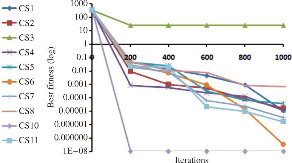
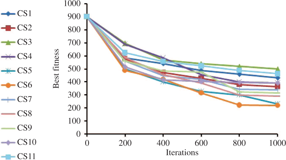
Figures 3–7 show the convergence behavior of five functions (f1, f2, f8, f12, f14) over 1000 iterations (with 50D size). In all of the figures, CS10 converges to a solution more quickly compared to the other CS variations. In contrast, CS3 has the worst convergence rate compared to the other CS variations.

Convergence Trend of f1.
Convergence Trend of f2.
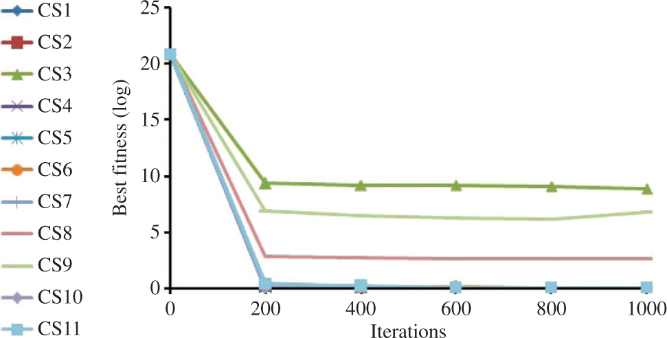
Convergence Trend of f8.
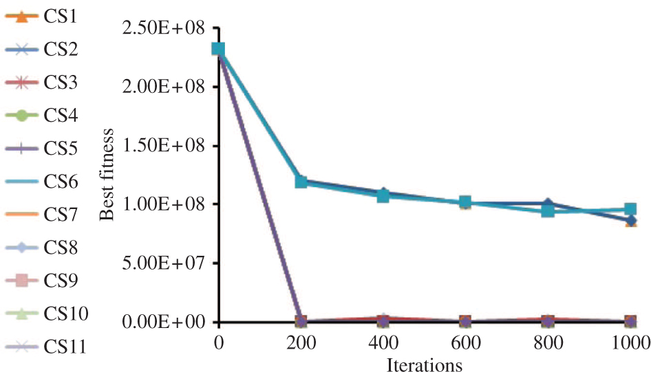
Convergence Trend of f12.
Convergence Trend of f14.
5.4 Statistical Test Results
As described in ref. [21], nonparametric statistical tests are the recommended methodology for comparing evolutionary algorithms. The Friedman test [23] has been used to test if the means of the 11 variations of CS are equal to determine if there exist at least two means that are significantly different from each other. The tested hypotheses are as follows:
H0:
H1: at least one mean is different from the others.
The results of the Friedman test for both 30 and 50 dimensions indicate that H1 should be accepted (p < 0.05) with results of 35.90 and 41.78, respectively. Furthermore, Tables 5 and 6 show results for the Conover post hoc test [15] for the different dimensions (Table 5: D = 30 and Table 6: D = 50). As can be seen from Table 5, for 30 dimensions, the results from CS3, CS4, CS9, and CS10 are significantly (p < 0.05) better than those for CS1. Similarly, from Table 6, the results from all variations except for CS7, CS8, and CS9 are significantly (p < 0.05) better than those for CS1. Combined with the analysis from the previous section, this suggests that CS10 is significantly better than CS1 while also converging more quickly. This suggests that the polynomial mutation could be a better mutation method than the Lévy flight method.
Conover Post hoc p-Value Matrix with 50 Runs and D = 30 for Tested Algorithms.
| CS1 | CS2 | CS3 | CS4 | CS5 | CS6 | CS7 | CS8 | CS9 | CS10 | CS11 | |
| CS1 | −1.00E+00 | 1.70E−01 | 7.39E−03 | 2.18E−02 | 9.75E−02 | 3.47E−01 | 8.28E−01 | 2.33E−01 | 4.80E−02 | 2.61E−02 | 7.17E−01 |
| CS2 | 1.70E−01 | −1.00E+00 | 7.22E−05 | 3.47E−01 | 7.72E−01 | 6.64E−01 | 1.13E−01 | 1.11E−02 | 9.75E−04 | 3.85E−01 | 3.12E−01 |
| CS3 | 7.39E−03 | 7.22E−05 | −1.00E+00 | 1.50E−06 | 2.32E−05 | 3.59E−04 | 1.35E−02 | 1.30E−01 | 4.69E−01 | 2.06E−06 | 2.49E−03 |
| CS4 | 2.18E−02 | 3.47E−01 | 1.50E−06 | −1.00E+00 | 5.15E−01 | 1.70E−01 | 1.23E−02 | 5.96E−04 | 3.10E−05 | 9.42E−01 | 5.22E−02 |
| CS5 | 9.75E−02 | 7.72E−01 | 2.32E−05 | 5.15E−01 | −1.00E+00 | 4.69E−01 | 6.14E−02 | 4.84E−03 | 3.59E−04 | 5.63E−01 | 1.94E−01 |
| CS6 | 3.47E−01 | 6.64E−01 | 3.59E−04 | 1.70E−01 | 4.69E−01 | −1.00E+00 | 2.48E−01 | 3.41E−02 | 3.89E−03 | 1.94E−01 | 5.63E−01 |
| CS7 | 8.28E−01 | 1.13E−01 | 1.35E−02 | 1.23E−02 | 6.14E−02 | 2.48E−01 | −1.00E+00 | 3.29E−01 | 7.77E−02 | 1.49E−02 | 5.63E−01 |
| CS8 | 2.33E−01 | 1.11E−02 | 1.30E−01 | 5.96E−04 | 4.84E−03 | 3.41E−02 | 3.29E−01 | −1.00E+00 | 4.26E−01 | 7.63E−04 | 1.21E−01 |
| CS9 | 4.80E−02 | 9.75E−04 | 4.69E−01 | 3.10E−05 | 3.59E−04 | 3.89E−03 | 7.77E−02 | 4.26E−01 | −1.00E+00 | 4.12E−05 | 1.98E−02 |
| CS10 | 2.61E−02 | 3.85E−01 | 2.06E−06 | 9.42E−01 | 5.63E−01 | 1.94E−01 | 1.49E−02 | 7.63E−04 | 4.12E−05 | −1.00E+00 | 6.14E−02 |
| CS11 | 7.17E−01 | 3.12E−01 | 2.49E−03 | 5.22E−02 | 1.94E−01 | 5.63E−01 | 5.63E−01 | 1.21E−01 | 1.98E−02 | 6.14E−02 | −1.00E+00 |
Non-diagonal values less than 0.05 are marked in bold.
Conover Post hoc p-Value Matrix with 50 Runs and D = 50 for Tested Algorithms.
| CS1 | CS2 | CS3 | CS4 | CS5 | CS6 | CS7 | CS8 | CS9 | CS10 | CS11 | |
| CS1 | −1.00E+00 | 8.13E−03 | 2.94E−02 | 2.38E−03 | 1.02E−03 | 1.50E−02 | 3.72E−01 | 3.92E−01 | 9.11E−01 | 3.78E−03 | 3.85E−02 |
| CS2 | 8.13E−03 | −1.00E+00 | 2.92E−06 | 6.82E−01 | 5.03E−01 | 8.23E−01 | 7.55E−02 | 5.43E−04 | 5.89E−03 | 7.94E−01 | 5.51E−01 |
| CS3 | 2.94E−02 | 2.92E−06 | −1.00E+00 | 4.79E−07 | 1.45E−07 | 7.52E−06 | 2.38E−03 | 1.81E−01 | 3.85E−02 | 9.33E−07 | 3.42E−05 |
| CS4 | 2.38E−03 | 6.82E−01 | 4.79E−07 | −1.00E+00 | 7.94E−01 | 5.27E−01 | 2.94E−02 | 1.24E−04 | 1.67E−03 | 8.82E−01 | 3.15E−01 |
| CS5 | 1.02E−03 | 5.03E−01 | 1.45E−07 | 7.94E−01 | −1.00E+00 | 3.72E−01 | 1.50E−02 | 4.58E−05 | 7.02E−04 | 6.82E−01 | 2.07E−01 |
| CS6 | 1.50E−02 | 8.23E−01 | 7.52E−06 | 5.27E−01 | 3.72E−01 | −1.00E+00 | 1.19E−01 | 1.16E−03 | 1.11E−02 | 6.28E−01 | 7.10E−01 |
| CS7 | 3.72E−01 | 7.55E−02 | 2.38E−03 | 2.94E−02 | 1.50E−02 | 1.19E−01 | −1.00E+00 | 8.17E−02 | 3.15E−01 | 4.21E−02 | 2.34E−01 |
| CS8 | 3.92E−01 | 5.43E−04 | 1.81E−01 | 1.24E−04 | 4.58E−05 | 1.16E−03 | 8.17E−02 | −1.00E+00 | 4.57E−01 | 2.15E−04 | 3.78E−03 |
| CS9 | 9.11E−01 | 5.89E−03 | 3.85E−02 | 1.67E−03 | 7.02E−04 | 1.11E−02 | 3.15E−01 | 4.57E−01 | −1.00E+00 | 2.68E−03 | 2.94E−02 |
| CS10 | 3.78E−03 | 7.94E−01 | 9.33E−07 | 8.82E−01 | 6.82E−01 | 6.28E−01 | 4.21E−02 | 2.15E−04 | 2.68E−03 | −1.00E+00 | 3.92E−01 |
| CS11 | 3.85E−02 | 5.51E−01 | 3.42E−05 | 3.15E−01 | 2.07E−01 | 7.10E−01 | 2.34E−01 | 3.78E−03 | 2.94E−02 | 3.92E−01 | −1.00E+00 |
Non-diagonal values less than 0.05 are marked in bold.
5.5 Comparison Results of CS with Other Algorithms
In this section, the CS algorithm was compared with the HS algorithm [26] and the ABC algorithm [22]. The algorithms were compared using eight different functions, F1, F3, F6, F10, F11, F12, F13, F14 for the following mutation methods: random mutation (M1 (random mutation), M2 (non-uniform random mutation with b = 1), M3 (non-uniform random mutation with b = 5), M4 (MPT mutation with b = 1), M5 (power mutation with b = 0.25), and M6 (polynomial mutation with b = 0.5)). The results for the ABC algorithm and the HS algorithm were taken from refs. [22], [26], respectively.
Simulation Results of CS, HS, and ABC Using Different Functions and Mutations.
| f(X) | M1 | M2 | M3 | M4 | M5 | M6 |
|---|---|---|---|---|---|---|
| F1 | 5.25E−07 | 1.15E−07 | 3.11E−08 | 2.81E−07 | 2.95E−05 | 0.00E+00 |
| I.739E+04 | 2.23E+04 | 2.4 90E+04 | I.636E+04 | 2.19E+04 | 5.82E−03 | |
| I.86E−15 | 1.86E−1 5 | 1.84E−15 | 1.86E−15 | 1.5BE−1 5 | 1.41E− 6 | |
| F3 | 0.00E+00 | 0.00E+00 | 0.00E+00 | 0.00E+00 | 4.58E+02 | 0.00E+00 |
| I.652E+04 | 2.03E+04 | 2.05E+04 | 1.58E+04 | J.922E+04 | 9.50E+00 | |
| 0.00E+00 | 0.00E+00 | 0.00E+00 | 0.00E+00 | 0.00E+00 | 0.00E+00 | |
| F6 | 5.87E+03 | 5.87E+03 | 5.87E+03 | 5.87E+03 | 6.10E+03 | 5.87E+03 |
| −3.58E+04 | −3.62E+04 | −3.62E+04 | −3.56E+04 | −2.93E+04 | −3.07E+04 | |
| −4.20E+04 | −4.20E+04 | −4.20E+04 | −4.20E+04 | −4.20E+04 | −4.20E+04 | |
| F10 | −1.03E+00 | −1.03E+00 | −1.03E+00 | −1.03E+00 | −1.03E+00 | −1.03E+00 |
| −1.03E+00 | −1.03E+00 | −1.03E+00 | −1.03E+00 | −1.03E+00 | −1.03E+00 | |
| −1.03E+00 | −1.03E+00 | −I.03E+00 | −I.03E+00 | −1.03E+00 | −I.03E+00 | |
| F11 | 3.72E+02 | 3.97E+02 | 3.84E+02 | 4.07E+02 | 5.63E+02 | 4.30E+02 |
| 2.301E+04 | 4.307E+04 | 1.30E+04 | 2.28E+04 | 3.35E+04 | −4.50E+02 | |
| −4.50E+02 | −4.50E+02 | −4.50E+02 | −4.50E+02 | −4.50E+02 | −4.50E+02 | |
| F12 | 9.22E+10 | 2.29E+11 | 1.18E+11 | 6.75E+10 | 3.52E+11 | 1.48E+11 |
| 3.79E+07 | 2.27E+07 | 2.25E+07 | 3.66E+07 | 1.11E+07 | 8.67E+07 | |
| −4.50E+02 | −4.50E+02 | −4.50E+02 | −4.50E+02 | −4.50E+02 | −4.50E+02 | |
| F13 | 1.90E+11 | 2.12E+11 | 1.30E+11 | 1.28E+11 | 2.51E+11 | 1.24E+11 |
| 3.03E+09 | 1.01E+09 | 9.97E+08 | 3.17E+09 | 7.06E+09 | 7.62E+04 | |
| 3.90E+02 | 3.90E+02 | 3.90E+02 | 3.90E+02 | 3.92E+02 | 3.90E+02 | |
| F14 | 1.17E+03 | 1.20E+03 | 1.39E+03 | 1.27E+03 | 1.14E+03 | 1.15E+03 |
| 4.58E+00 | 6.32E+01 | 5.18E+01 | 6.55E+00 | 4.979E+O1 | 1.02E+02 | |
| −3.30E+02 | −3.30E+02 | −3.30E+02 | −3.30E+02 | −3.30E+02 | −3.00E+02 |
The mean of 50 runs is shown. CS results are in the first row for each function.
The best results are marked with bold.
Table 7 shows the mean values of the objective values of CS, ABC, and HS over 50 independent runs for 100D problems. The results are in the following format: CS results in the first row, HS results in the second row, and ABC results in the third row for each function. The table illustrates that the variations of CS show competitive performance compared to the variations of ABC and HS. However, the variations of the ABC algorithm outperform the other algorithms for five functions out of eight. Nevertheless, the obtained results for the three algorithms confirm that the performance of the optimization algorithms is affected by the type of the chosen mutation method.
6 Conclusion
The current paper presented new variations of CS using different mutation methods. Extensive simulations were conducted using a set of 14 well-known benchmark functions to evaluate the performance of the proposed variations of CS. CS with polynomial mutation was found to be more accurate and stable than the other algorithms for a notable number of the benchmark functions.
Future work will be directed towards implementing different selection schemes to CS with polynomial mutation instead of the currently used random selection method. Future work also includes hybridizing CS with polynomial mutation and the simulated annealing algorithm [13]. Furthermore, it would be interesting to see how CS with polynomial mutation performs in practice when it is applied to cooperative Q-learning [1], [9], [10], [11], as described in refs. [2], [3].
Bibliography
[1] B. H. K. Abed-alguni, Cooperative reinforcement learning for independent learners, PhD thesis, Faculty of Engineering and Built Environment, School of Electrical Engineering and Computer Science, The University of Newcastle, Australia, 2014.Search in Google Scholar
[2] B. H. Abed-alguni, Action-selection method for reinforcement learning based on cuckoo search algorithm, Arabian J. Sci. Eng. (2017), 1–15. https://doi.org/10.1007/s13369-017-2873-8.10.1007/s13369-017-2873-8Search in Google Scholar
[3] B. H. Abed-alguni, Bat Q-learning algorithm, Jordanian J. Comput. Inf. Technol. (JJCIT) 3 (2017), 56–77.10.5455/jjcit.71-1480540385Search in Google Scholar
[4] B. H. Abed-alguni, Island-based cuckoo search with highly disruptive polynomial mutatio, Int. J. Artif. Intelligence 8 (2019), 1–30.Search in Google Scholar
[5] B. H. Abed-alguni and F. Alkhateeb, Novel selection schemes for cuckoo search, Arabian J. Sci. Eng. 42 (2017), 3635–3654.10.1007/s13369-017-2663-3Search in Google Scholar
[6] B. H. Abed-alguni and F. Alkhateeb, Intelligent hybrid cuckoo search and β-hill climbing algorithm, J. King Saud University – Comput. Inf. Sci. 0 (2018), 1–43.10.1016/j.jksuci.2018.05.003Search in Google Scholar
[7] B. H. Abed-alguni and M. Barhoush, Distributed grey wolf optimizer for numerical optimization problems, Jordanian J. Comput. Inf. Technol. (JJCIT) 4 (2018), 130–149.Search in Google Scholar
[8] B. H. Abed-alguni and A. F. Klaib, Hybrid whale optimization and β-hill climbing algorithm, Int. J. Comput. Sci. Mathematics 0 (2018), 1–13.Search in Google Scholar
[9] B. H. Abed-alguni and M. A. Ottom, Double delayed Q-learning, Int. J. Artif. Intelligence 16 (2018), 41–59.Search in Google Scholar
[10] B. H. Abed-alguni, S. K. Chalup, F. A. Henskens and D. J. Paul, A multi-agent cooperative reinforcement learning model using a hierarchy of consultants, tutors and workers, Vietnam J. Comput. Sci. 2 (2015), 213–226.10.1007/s40595-015-0045-xSearch in Google Scholar
[11] B. H. Abed-alguni, S. K. Chalup, F. A. Henskens and D. J. Paul, Erratum to: a multi-agent cooperative reinforcement learning model using a hierarchy of consultants, tutors and workers, Vietnam J. Comput. Sci. 2 (2015), 227–227.10.1007/s40595-015-0047-8Search in Google Scholar
[12] B. H. Abed-alguni, D. J. Paul, S. K. Chalup and F. A. Henskens, A comparison study of cooperative Q-learning algorithms for independent learners, Int. J. Artif. Intelligence 14 (2016), 71–93.Search in Google Scholar
[13] F. Alkhateeb and B. H. Abed-alguni, A hybrid cuckoo search and simulated annealing algorithm, J. Intelligent Syst. 28 (2017), 683–698.10.1515/jisys-2017-0268Search in Google Scholar
[14] L. T. Bui and H. Thi Thanh Binh, A survivable design of last mile communication networks using multi-objective genetic algorithms, Memetic Computing 8 (2016), 97–108.10.1007/s12293-015-0177-7Search in Google Scholar
[15] W. Conover and R. L. Iman, On multiple-comparisons procedures, Los Alamos Sci. Lab. Tech. Rep. LA-7677-MS (1979), 1–14.10.2172/6057803Search in Google Scholar
[16] Z. Cui, B. Sun, G. Wang, Y. Xue and J. Chen, A novel oriented cuckoo search algorithm to improve dv-hop performance for cyber–physical systems, J. Parallel Distrib. Comput. 103 (2017), 42–52.10.1016/j.jpdc.2016.10.011Search in Google Scholar
[17] K. Deb and R. B. Agrawal, Simulated binary crossover for continuous search space, Complex Syst. 9 (1994), 1–15.Search in Google Scholar
[18] K. Deb and S. Tiwari, Omni-optimizer: a generic evolutionary algorithm for single and multi-objective optimization, Eur. J. Operational Res. 185 (2008), 1062–1087.10.1016/j.ejor.2006.06.042Search in Google Scholar
[19] K. Deb, A. Pratap, S. Agarwal and T. Meyarivan, A fast and elitist multiobjective genetic algorithm: Nsga-ii, IEEE Trans. Evolutionary Comput. 6 (2002), 182–197.10.1109/4235.996017Search in Google Scholar
[20] K. Deep and M. Thakur, A new mutation operator for real coded genetic algorithms, Appl. Mathematics Comput. 193 (2007), 211–230.10.1016/j.amc.2007.03.046Search in Google Scholar
[21] J. Derrac, S. Garca, D. Molina and F. Herrera, A practical tutorial on the use of nonparametric statistical tests as a methodology for comparing evolutionary and swarm intelligence algorithms, Swarm Evolutionary Comput. 1 (2011), 3–18.10.1016/j.swevo.2011.02.002Search in Google Scholar
[22] I. A. Doush, B. H. F. Hasan, M. A. Al-Betar, E. Al Maghayreh, F. Alkhateeb and M. Hamdan, Artificial bee colony with different mutation schemes: a comparative study, Comput. Sci. J. Moldova 22 (2014), 77–98.Search in Google Scholar
[23] M. Friedman, A comparison of alternative tests of significance for the problem of m rankings, Ann. Math. Statistics 11 (1940), 86–92.10.1214/aoms/1177731944Search in Google Scholar
[24] A. H. Gandomi and A. H. Alavi, Krill herd: a new bio-inspired optimization algorithm, Commun. Nonlinear Sci. Numer. Simul. 17 (2012), 4831–4845.10.1016/j.cnsns.2012.05.010Search in Google Scholar
[25] Z. W. Geem, J. H. Kim and G. Loganathan, A new heuristic optimization algorithm: harmony search, Simulation 76 (2001), 60–68.10.1177/003754970107600201Search in Google Scholar
[26] B. H. F. Hasan, I. A. Doush, E. Al Maghayreh, F. Alkhateeb and M. Hamdan, Hybridizing harmony search algorithm with different mutation operators for continuous problems, Appl. Mathematics Comput. 232 (2014), 1166–1182.10.1016/j.amc.2013.12.139Search in Google Scholar
[27] G. Kanagaraj, S. Ponnambalam and N. Jawahar, A hybrid cuckoo search and genetic algorithm for reliability – redundancy allocation problems, Comput. Ind. Eng. 66 (2013), 1115–1124.10.1016/j.cie.2013.08.003Search in Google Scholar
[28] G. Kanagaraj, S. Ponnambalam, N. Jawahar and J. M. Nilakantan, An effective hybrid cuckoo search and genetic algorithm for constrained engineering design optimization, Eng. Optimization 46 (2014), 1331–1351.10.1080/0305215X.2013.836640Search in Google Scholar
[29] S. Kundu and D. R. Parhi, Navigation of underwater robot based on dynamically adaptive harmony search algorithm, Memetic Comput. 8 (2016), 125–146.10.1007/s12293-016-0179-0Search in Google Scholar
[30] H.-w. Lin, Y. Wang and C. Dai, A swarm intelligence algorithm based on boundary mutation, in: Computational Intelligence and Security (CIS), 2010 International Conference, Nanning, Guangxi Zhuang Autonomous Region, China, pp. 195–199, IEEE, 2010.10.1109/CIS.2010.48Search in Google Scholar
[31] Z. Michalewicz, Genetic algorithms + data structures =evolution programs, 2nd extended ed., Springer-Verlag New York, Inc., New York, NY, USA, 1994.10.1007/978-3-662-07418-3Search in Google Scholar
[32] Z. Michalewicz, T. Logan and S. Swaminathan, Evolutionary operators for continuous convex parameter spaces, in: Proceedings of the 3rd Annual conference on Evolutionary Programming, University of California, San Diego, USA, pp. 84–97, World Scientific, 1994.Search in Google Scholar
[33] S. Mirjalili and A. Lewis, The whale optimization algorithm, Adv. Eng. Software 95 (2016), 51–67.10.1016/j.advengsoft.2016.01.008Search in Google Scholar
[34] P. K. Mohanty and D. R. Parhi, A new hybrid optimization algorithm for multiple mobile robots navigation based on the CS-ANFIS approach, Memetic Comput. 7 (2015), 255–273.10.1007/s12293-015-0160-3Search in Google Scholar
[35] H. Rakhshani and A. Rahati, Intelligent multiple search strategy cuckoo algorithm for numerical and engineering optimization problems, Arabian J. Sci. Eng. 42 (2016), 1–27.10.1007/s13369-016-2270-8Search in Google Scholar
[36] M. Saraswathi, G. B. Murali and B. Deepak, Optimal path planning of mobile robot using hybrid cuckoo search-bat algorithm, Procedia Comput. Sci. 133 (2018), 510–517.10.1016/j.procs.2018.07.064Search in Google Scholar
[37] J. Toivanen, R. Makinen, J. Périaux and F. Cloud Cedex, Multidisciplinary shape optimization in aerodynamics and electromagnetics using genetic algorithms, Intl J. Numer. Meth. Fluids 30 (1999), 149–159.10.1002/(SICI)1097-0363(19990530)30:2<149::AID-FLD829>3.0.CO;2-BSearch in Google Scholar
[38] H. Wang and J.-H. Yi, An improved optimization method based on krill herd and artificial bee colony with information exchange, Memetic Comput. 10 (2018), 177–198.10.1007/s12293-017-0241-6Search in Google Scholar
[39] G. Wang, L. Guo, A. H. Gandomi, L. Cao, A. H. Alavi, H. Duan and J. Li, Lévy-flight krill herd algorithm, Math. Problems Eng. 2013 (2013), 1–14.10.1155/2013/682073Search in Google Scholar
[40] G.-G. Wang, A. H. Gandomi, X.-S. Yang and A. H. Alavi, A new hybrid method based on krill herd and cuckoo search for global optimisation tasks, Int. J. Bio-Inspired Comput. 8 (2016), 286–299.10.1504/IJBIC.2016.079569Search in Google Scholar
[41] G.-G. Wang, A. H. Gandomi, X. Zhao and H. C. E. Chu, Hybridizing harmony search algorithm with cuckoo search for global numerical optimization, Soft Comput. 20 (2016), 273–285.10.1007/s00500-014-1502-7Search in Google Scholar
[42] X.-S. Yang and S. Deb, Cuckoo search via lévy flights, in: World Congress on Nature & Biologically Inspired Computing, 2009. NaBIC 2009, pp. 210–214, IEEE, 2009.10.1109/NABIC.2009.5393690Search in Google Scholar
[43] X.-S. Yang and S. Deb, Engineering optimisation by cuckoo search, Int. J. Math. Modell. Numer. Optimisation 1 (2010), 330–343.10.1504/IJMMNO.2010.035430Search in Google Scholar
[44] M. Zhang, H. Wang, Z. Cui and J. Chen, Hybrid multi-objective cuckoo search with dynamical local search, Memetic Comput. 10 (2017), 199–208.10.1007/s12293-017-0237-2Search in Google Scholar
©2020 Walter de Gruyter GmbH, Berlin/Boston
This work is licensed under the Creative Commons Attribution 4.0 Public License.
Articles in the same Issue
- An Optimized K-Harmonic Means Algorithm Combined with Modified Particle Swarm Optimization and Cuckoo Search Algorithm
- Texture Feature Extraction Using Intuitionistic Fuzzy Local Binary Pattern
- Leaf Disease Segmentation From Agricultural Images via Hybridization of Active Contour Model and OFA
- Deadline Constrained Task Scheduling Method Using a Combination of Center-Based Genetic Algorithm and Group Search Optimization
- Efficient Classification of DDoS Attacks Using an Ensemble Feature Selection Algorithm
- Distributed Multi-agent Bidding-Based Approach for the Collaborative Mapping of Unknown Indoor Environments by a Homogeneous Mobile Robot Team
- An Efficient Technique for Three-Dimensional Image Visualization Through Two-Dimensional Images for Medical Data
- Combined Multi-Agent Method to Control Inter-Department Common Events Collision for University Courses Timetabling
- An Improved Particle Swarm Optimization Algorithm for Global Multidimensional Optimization
- A Kernel Probabilistic Model for Semi-supervised Co-clustering Ensemble
- Pythagorean Hesitant Fuzzy Information Aggregation and Their Application to Multi-Attribute Group Decision-Making Problems
- Using an Efficient Optimal Classifier for Soil Classification in Spatial Data Mining Over Big Data
- A Bayesian Multiresolution Approach for Noise Removal in Medical Magnetic Resonance Images
- Gbest-Guided Artificial Bee Colony Optimization Algorithm-Based Optimal Incorporation of Shunt Capacitors in Distribution Networks under Load Growth
- Graded Soft Expert Set as a Generalization of Hesitant Fuzzy Set
- Universal Liver Extraction Algorithm: An Improved Chan–Vese Model
- Software Effort Estimation Using Modified Fuzzy C Means Clustering and Hybrid ABC-MCS Optimization in Neural Network
- Handwritten Indic Script Recognition Based on the Dempster–Shafer Theory of Evidence
- An Integrated Intuitionistic Fuzzy AHP and TOPSIS Approach to Evaluation of Outsource Manufacturers
- Automatically Assess Day Similarity Using Visual Lifelogs
- A Novel Bio-Inspired Algorithm Based on Social Spiders for Improving Performance and Efficiency of Data Clustering
- Discriminative Training Using Noise Robust Integrated Features and Refined HMM Modeling
- Self-Adaptive Mussels Wandering Optimization Algorithm with Application for Artificial Neural Network Training
- A Framework for Image Alignment of TerraSAR-X Images Using Fractional Derivatives and View Synthesis Approach
- Intelligent Systems for Structural Damage Assessment
- Some Interval-Valued Pythagorean Fuzzy Einstein Weighted Averaging Aggregation Operators and Their Application to Group Decision Making
- Fuzzy Adaptive Genetic Algorithm for Improving the Solution of Industrial Optimization Problems
- Approach to Multiple Attribute Group Decision Making Based on Hesitant Fuzzy Linguistic Aggregation Operators
- Cubic Ordered Weighted Distance Operator and Application in Group Decision-Making
- Fault Signal Recognition in Power Distribution System using Deep Belief Network
- Selector: PSO as Model Selector for Dual-Stage Diabetes Network
- Oppositional Gravitational Search Algorithm and Artificial Neural Network-based Classification of Kidney Images
- Improving Image Search through MKFCM Clustering Strategy-Based Re-ranking Measure
- Sparse Decomposition Technique for Segmentation and Compression of Compound Images
- Automatic Genetic Fuzzy c-Means
- Harmony Search Algorithm for Patient Admission Scheduling Problem
- Speech Signal Compression Algorithm Based on the JPEG Technique
- i-Vector-Based Speaker Verification on Limited Data Using Fusion Techniques
- Prediction of User Future Request Utilizing the Combination of Both ANN and FCM in Web Page Recommendation
- Presentation of ACT/R-RBF Hybrid Architecture to Develop Decision Making in Continuous and Non-continuous Data
- An Overview of Segmentation Algorithms for the Analysis of Anomalies on Medical Images
- Blind Restoration Algorithm Using Residual Measures for Motion-Blurred Noisy Images
- Extreme Learning Machine for Credit Risk Analysis
- A Genetic Algorithm Approach for Group Recommender System Based on Partial Rankings
- Improvements in Spoken Query System to Access the Agricultural Commodity Prices and Weather Information in Kannada Language/Dialects
- A One-Pass Approach for Slope and Slant Estimation of Tri-Script Handwritten Words
- Secure Communication through MultiAgent System-Based Diabetes Diagnosing and Classification
- Development of a Two-Stage Segmentation-Based Word Searching Method for Handwritten Document Images
- Pythagorean Fuzzy Einstein Hybrid Averaging Aggregation Operator and its Application to Multiple-Attribute Group Decision Making
- Ensembles of Text and Time-Series Models for Automatic Generation of Financial Trading Signals from Social Media Content
- A Flame Detection Method Based on Novel Gradient Features
- Modeling and Optimization of a Liquid Flow Process using an Artificial Neural Network-Based Flower Pollination Algorithm
- Spectral Graph-based Features for Recognition of Handwritten Characters: A Case Study on Handwritten Devanagari Numerals
- A Grey Wolf Optimizer for Text Document Clustering
- Classification of Masses in Digital Mammograms Using the Genetic Ensemble Method
- A Hybrid Grey Wolf Optimiser Algorithm for Solving Time Series Classification Problems
- Gray Method for Multiple Attribute Decision Making with Incomplete Weight Information under the Pythagorean Fuzzy Setting
- Multi-Agent System Based on the Extreme Learning Machine and Fuzzy Control for Intelligent Energy Management in Microgrid
- Deep CNN Combined With Relevance Feedback for Trademark Image Retrieval
- Cognitively Motivated Query Abstraction Model Based on Associative Root-Pattern Networks
- Improved Adaptive Neuro-Fuzzy Inference System Using Gray Wolf Optimization: A Case Study in Predicting Biochar Yield
- Predict Forex Trend via Convolutional Neural Networks
- Optimizing Integrated Features for Hindi Automatic Speech Recognition System
- A Novel Weakest t-norm based Fuzzy Fault Tree Analysis Through Qualitative Data Processing and Its Application in System Reliability Evaluation
- FCNB: Fuzzy Correlative Naive Bayes Classifier with MapReduce Framework for Big Data Classification
- A Modified Jaya Algorithm for Mixed-Variable Optimization Problems
- An Improved Robust Fuzzy Algorithm for Unsupervised Learning
- Hybridizing the Cuckoo Search Algorithm with Different Mutation Operators for Numerical Optimization Problems
- An Efficient Lossless ROI Image Compression Using Wavelet-Based Modified Region Growing Algorithm
- Predicting Automatic Trigger Speed for Vehicle-Activated Signs
- Group Recommender Systems – An Evolutionary Approach Based on Multi-expert System for Consensus
- Enriching Documents by Linking Salient Entities and Lexical-Semantic Expansion
- A New Feature Selection Method for Sentiment Analysis in Short Text
- Optimizing Software Modularity with Minimum Possible Variations
- Optimizing the Self-Organizing Team Size Using a Genetic Algorithm in Agile Practices
- Aspect-Oriented Sentiment Analysis: A Topic Modeling-Powered Approach
- Feature Pair Index Graph for Clustering
- Tangramob: An Agent-Based Simulation Framework for Validating Urban Smart Mobility Solutions
- A New Algorithm Based on Magic Square and a Novel Chaotic System for Image Encryption
- Video Steganography Using Knight Tour Algorithm and LSB Method for Encrypted Data
- Clay-Based Brick Porosity Estimation Using Image Processing Techniques
- AGCS Technique to Improve the Performance of Neural Networks
- A Color Image Encryption Technique Based on Bit-Level Permutation and Alternate Logistic Maps
- A Hybrid of Deep CNN and Bidirectional LSTM for Automatic Speech Recognition
- Database Creation and Dialect-Wise Comparative Analysis of Prosodic Features for Punjabi Language
- Trapezoidal Linguistic Cubic Fuzzy TOPSIS Method and Application in a Group Decision Making Program
- Histopathological Image Segmentation Using Modified Kernel-Based Fuzzy C-Means and Edge Bridge and Fill Technique
- Proximal Support Vector Machine-Based Hybrid Approach for Edge Detection in Noisy Images
- Early Detection of Parkinson’s Disease by Using SPECT Imaging and Biomarkers
- Image Compression Based on Block SVD Power Method
- Noise Reduction Using Modified Wiener Filter in Digital Hearing Aid for Speech Signal Enhancement
- Secure Fingerprint Authentication Using Deep Learning and Minutiae Verification
- The Use of Natural Language Processing Approach for Converting Pseudo Code to C# Code
- Non-word Attributes’ Efficiency in Text Mining Authorship Prediction
- Design and Evaluation of Outlier Detection Based on Semantic Condensed Nearest Neighbor
- An Efficient Quality Inspection of Food Products Using Neural Network Classification
- Opposition Intensity-Based Cuckoo Search Algorithm for Data Privacy Preservation
- M-HMOGA: A New Multi-Objective Feature Selection Algorithm for Handwritten Numeral Classification
- Analogy-Based Approaches to Improve Software Project Effort Estimation Accuracy
- Linear Regression Supporting Vector Machine and Hybrid LOG Filter-Based Image Restoration
- Fractional Fuzzy Clustering and Particle Whale Optimization-Based MapReduce Framework for Big Data Clustering
- Implementation of Improved Ship-Iceberg Classifier Using Deep Learning
- Hybrid Approach for Face Recognition from a Single Sample per Person by Combining VLC and GOM
- Polarity Analysis of Customer Reviews Based on Part-of-Speech Subcategory
- A 4D Trajectory Prediction Model Based on the BP Neural Network
- A Blind Medical Image Watermarking for Secure E-Healthcare Application Using Crypto-Watermarking System
- Discriminating Healthy Wheat Grains from Grains Infected with Fusarium graminearum Using Texture Characteristics of Image-Processing Technique, Discriminant Analysis, and Support Vector Machine Methods
- License Plate Recognition in Urban Road Based on Vehicle Tracking and Result Integration
- Binary Genetic Swarm Optimization: A Combination of GA and PSO for Feature Selection
- Enhanced Twitter Sentiment Analysis Using Hybrid Approach and by Accounting Local Contextual Semantic
- Cloud Security: LKM and Optimal Fuzzy System for Intrusion Detection in Cloud Environment
- Power Average Operators of Trapezoidal Cubic Fuzzy Numbers and Application to Multi-attribute Group Decision Making