Predicting Automatic Trigger Speed for Vehicle-Activated Signs

Diala Jomaa; Siril Yella

doi:10.1515/jisys-2016-0329

Article Open Access

Predicting Automatic Trigger Speed for Vehicle-Activated Signs

Diala Jomaa and Siril Yella

Published/Copyright: November 16, 2018

Published by

Become an author with De Gruyter Brill

Submit Manuscript Author Information

From the journal Journal of Intelligent Systems Volume 29 Issue 1

Abstract

Vehicle-activated signs (VAS) are speed-warning signs activated by radar when the driver speed exceeds a pre-set threshold, i.e. the trigger speed. The trigger speed is often set relative to the speed limit and is displayed for all types of vehicles. It is our opinion that having a static setting for the trigger speed may be inappropriate, given that traffic and road conditions are dynamic in nature. Further, different vehicle classes (mainly cars and trucks) behave differently, so a uniform trigger speed of such signs may be inappropriate to warn different types of vehicles. The current study aims to investigate an automatic VAS, i.e. one that could warn vehicle users with an appropriate trigger speed by taking into account vehicle types and road conditions. We therefore investigated different vehicle classes, their speeds, and the time of day to be able to conclude whether different trigger speeds of VAS are essential or not. The current study is entirely data driven; data are initially presented to a self-organising map (SOM) to be able to partition the data into different clusters, i.e. vehicle classes. Speed, time of day, and length of vehicle were supplied as inputs to the SOM. Further, the 85th percentile speed for the next hour is predicted using appropriate prediction models. Adaptive neuro-fuzzy inference systems and random forest (RF) were chosen for speed prediction; the mean speed, traffic flow, and standard deviation of vehicle speeds were supplied as inputs for the prediction models. The results achieved in this work show that RF is a reliable model in terms of accuracy and efficiency, and can be used in finding appropriate trigger speeds for an automatic VAS.

Keywords: Vehicle-activated signs; adaptive neuro-fuzzy inference systems; random forest; self-organising maps; trigger speed

1 Introduction

Speed and speed variance are two common factors affecting the frequency and severity of traffic accidents. Reducing speed and speed variance are key objectives for reducing both the frequency and severity of crashes. One way to do this is to use vehicle-activated signs (VAS), which are warning signs that display a warning message “reduce speed” with the posted speed limit. The trigger speed is often set relative to the speed limit and is displayed for all types of vehicles. Given the size, weight, and behavioural differences between motorcycles, cars, and trucks, having a uniform trigger speed for such sign may be inappropriate to warn different vehicle types. This study was conducted to examine the necessity of triggering VAS respective to the type of vehicle. This issue is, however, connected to the general problem in setting the appropriate speed limit on a road segment and the challenge of using uniform and differential speed limit (DSL) strategies. DSL is a speed control strategy aimed to address different speed limits for cars and trucks. A number of authorities have encountered this general problem and used the DSL strategies by either setting the maximum speed for trucks at a certain threshold value, such as 10–15 km/h lower than for cars or by requiring all trucks to be equipped with maximum speed limiters [9], [13], [18]. The safety effects of such settings have not been conclusive in previous studies. Some studies found no difference between DSL and uniform speed limit for cars and trucks [7], [11], [12], [14]. Other studies found that DSL can be better policy choice [6], [10]. The differences between the studies could be based on the difference in the thresholds applied in the DSL, but can also be attributed to varying factors such as weather, traffic, and road conditions. The current study aims to investigate an automatic VAS, i.e. one that could warn vehicle users with an appropriate trigger speed by taking into account vehicle types and road conditions. Traffic speed data were collected from four test sites in Sweden. A data-driven methodology has been chosen for the purpose. A data-driven model is able to mitigate the aforementioned problems encountered while investigating DSL; further, such a model is immune to any external influences such as decisions made by authorities and so on.

A large number of input factors that impact the current traffic situations have frequently been considered in relevant studies [25], [26]. Such input factors, including time/day, flow of traffic (i.e. number of vehicles for a certain period of time), mean speeds, and standard deviation, are usually examined in the previous literature. Besides, traffic situations may change or repeat intensively depending on the time of day and day of the week [20]. In other words, the input factors may have similar patterns in rush/non-rush hours on different days of the week. Although past studies have extensively researched the above-mentioned factors relevant to traffic situations, fewer studies have attempted to deal with the type of vehicles in particular, applying DSL strategies to be able to trigger a VAS.

The first objective of this paper is to study the difference in mean speeds and standard deviations between all types of vehicles, particularly motorcycles, cars, trucks, and long trucks, and between the times of day (particularly night time and day time). Hypothesis testing was used to prove whether there were differences in mean speed and standard deviation within the vehicle classes and time of day [5]. A second objective is to present an automatic trigger speed for VAS responding automatically to traffic conditions. The automatic system will first use a self-organising map (SOM) to partition the input data into separate clusters that have similar traffic patterns and then predict the 85th percentile trigger speed within each cluster.

SOM is capable of finding features inherent to the problem without the need for prior determination of the output, and is therefore appropriate in a data-driven study. Two different predictive models, namely random forest (RF) and adaptive neuro-fuzzy system (ANFIS), were chosen to automate the trigger speed of the VAS.

The rest of the paper is organised as follows: Section 2 presents a description of the theoretical background of the different methodologies used in this study. Section 3 describes the data collection. Data analysis is reported in Section 4. The automatic trigger speed models are presented in Section 5. Section 6 summarises and concludes the study.

2 Theoretical Background

A brief description of the models employed in this work has been provided for the benefit of the reader unfamiliar with the topic.

2.1 Self-Organising Maps

SOM is one of the most popular neural network models used in clustering [20]. SOM has been proven useful in many applications [4], [24], [27], [28]. SOM is based on unsupervised learning, which means that no human intervention is needed during the learning process, and there is little need to know about the characteristics of the input data and no need to know which membership class the input class belongs to. SOM belongs to the category of competitive learning networks. The goal of learning in SOM is to cause different parts of the network to respond similarly to certain input patterns. It consists of two layers of artificial neurons: an input layer and an output layer. Every input neuron is connected to every output neuron by a weighting value. The Euclidian distance is calculated between the input vector and the incoming weighted vector for each output. The output neuron with the smallest distance is declared as the winner, and its weights are modified to be closer to the input vector. In fact, SOM is an iterative process where the connections’ weights are modified according to the following equations:

(1) w(t+1)=w(t)+h(t)(x(t)−w(t)),

(2) h(t)=α⋅e− d22σ2(t),

where w(t) is the connection weight at time t, x(t) is the input vector, h(t) is the neighbourhood function, α is the learning rate, d is the Euclidian distance between the winning unit and the current unit, and σ is the neighbourhood width parameter.

In this paper, an SOM was initially used to visualise and understand data properties such as the number of prevalent clusters. A complete discussion concerning SOM is beyond the scope of this article but can be found elsewhere [20].

2.2 Adaptive Neuro-Fuzzy System

An adaptive neuro-fuzzy system is a powerful system that combines the concepts of two approaches into one integrated system where artificial neural network learning algorithms are used to determine the parameters of the fuzzy inference system to share data structures and knowledge representations. In this paper, the fuzzy inference system is based on the Takagi-Sugeno methodology where the output membership functions are constant values. After some experimentation, a bell-shaped function has been chosen as the main membership function for the inputs. Bearing in mind the smooth nature and also the fact that it allows for a greater interval, i.e. the interval where μ(x)=1, in this study, the membership function is given as follows:

(3) μAi=11+(x−ciai)2bi, μBi=11+(y−ciai)2bi,

and a typical rule in this Sugeno method is also as follows:

(4) If x=Ai and by=Bi thenoutput is z=ax+by+c.

where μAi and μBi are membership functions for fuzzy sets A and B for node i. x is the first input; y is the second input; A_{_i} and B_{_i} are the fuzzy sets; z is the output obtained by the fuzzy rule; and a_{_i} , b_{_i} , and c_{_i} are the parameters of membership functions for node i called conditional parameters, and determined during the training process.

A typical ANFIS structure, first proposed by Jang [16], [17], [22], is a network of five layers of nodes (see Figure 1). A brief description of each layer is as follows:

Figure 1:

ANFIS Structure with Five Nodes, Two Inputs, and One Single Output [16].

Layer 1 – In this layer, every node is a fuzzy set and the output of any node corresponds to the membership function in this fuzzy set.
Layer 2 – Every node computes the degree of activation w_i of rule i where the membership functions are multiplied by the AND operator as follows:

(5) wi=μAi(x)μBi(y).
Layer 3 – The third layer computes the ratio of the activity degree of i rule to the sum of activation degrees of all rules. W_i is consequently considered as the normalised membership degree of i rule [see Eq. (6)].

(6) Wi=wiw1+w2.
Layer 4 – The node function of the fourth layer computes the contribution of each i rule towards the total output, and the function f_i defined as in Eq. (7):

(7) Wifi=Wi(aix+biy+ci).
Layer 5 – The final outputs of all nodes are derived in this final layer [see Eq. (8)].

(8) ∑Wifi=∑wifi/∑wi.

The network is trained using a hybrid learning algorithm based on two steps. In the first step (forward pass), the premise parameters (i.e. network parameters) are kept fixed and the information is propagated forwards in the network using the least-square method to identify the consequent parameters for the current cycle through training. In the second step (backward pass), the error is propagated backwards, while the premise parameters are modified using the gradient descent method by keeping the consequent parameters fixed. The rule extraction method first uses the fuzzy c-means (FCM) clustering function known as “genfis3” to determine the number of rules and membership functions for the antecedents and consequents. FCM clustering techniques (genfis3) were also used to optimise the result by extracting a set of rules that model the data and generate an initial FIS for ANFIS training.

2.3 Random Forest

An RF is an ensemble machine learning proposed by Leo Breiman for building tree predictors and letting them vote for the most popular class. The algorithm of inducing RF is based on bootstrap aggregation or so-called bagging. RF is a refinement of bagged trees. For bagging, given a training set X=x₁, …, x_{_n} with response variables Y=y₁, …, y_{_n} , the algorithm selects a random sample with replacement of the training set and fits tree regressions to these samples. After training, predictions can be made by averaging the predictions from all individual regression trees. The latter improves the stability and accuracy of machine learning algorithms, particularly used in statistical classification and regression [1]. It also reduces variance and helps avoid overfitting. RFs differ in only one way from the general bagging process. The algorithm uses a modified tree learning algorithm that selects, at each candidate split in the learning process, a random subset of the features. This process is also called feature bagging. The reason for this is to overcome the correlation of the trees from an ordinary bootstrap sample. In other words, RF tries to improve on bagging by “de-correlating” the trees. A detailed description can be found in Refs. [2], [15]. The RF algorithm is summarised as follows:

Draw ntree bootstrap samples from the original data.
For each of the bootstrap samples, draw a random sample of m features, and those m features are considered for each tree split. Typically, m=p or log2 p, where p is the number of features.
Predict new data by aggregating the predictions of the ntree trees (i.e. majority votes for classification, average for regression).
Calculate the error rate for observations left out of the bootstrap sample. This is called the out-of-bag error rate.

For the implementation of the RF in this paper, the number of trees and the number of selected features were experimentally tuned. As the number of trees increases, the error converges to a limit where there is no presence of overfitting, as in the case of multilayer perceptron and other learning algorithms. The most important parameter is to decide upon the number of features to test at each split. A common practice is to start with a large number and then either increase or decrease the number of features until the minimum error for the prediction is obtained.

3 Data

Traffic speed data were collected 24 h a day, onsite at four different locations. The first site (site-1: latitude: 60.558988, longitude: 15.137701) was located on highway E16 between Borlänge and Djurås in central Sweden and was restricted to 60 km/h. The second (site-2: latitude: 60.476904, longitude: 15.464145) and third (site-3: latitude: 60.462058, longitude: 15.467076) sites were both restricted to 40 km/h, whereas the fourth site (site-4: latitude: 60.497165, longitude: 15.452249) was restricted to 60 km/h. One single VAS was used to collect all the data from the different sites to keep costs low. Further details such as the number of observations and dates can be found in Table 1. At this stage, it is worth mentioning that the VAS was equipped with radar and a data logger to record the speed of passing vehicles 100 m before the location of the VAS. The rationale behind such a VAS was to build an adaptive VAS that detects and records vehicle speeds, and predicts a trigger speed respective to previous traffic conditions.

Table 1:

Data Description, Number of Observations in the Original Data Set, Mean Speed, 85th Percentile, and Standard Deviation for Each Vehicle Class.

Site	Classes	Observations	Mean speed (km/h)	85th percentile (km/h)	Standard deviation
1	C1	34,673	59.4	74	19.1
	C2	175,822	63.9	73	11.7
	C3	15,258	63.4	72	11
	C4	13,373	64	73	11.2
2	C1	2127	32.6	52	17.54
	C2	54,116	48.5	58	9.94
	C3	4019	38.5	53	15.1
	C4	3494	32.7	48	14.4
3	C1	702	42.1	54	14.3
	C2	50,388	47.5	56	8.82
	C3	5361	46.9	56	8.81
	C4	2107	44.3	52	8.45
4	C1	11,021	35.3	56	19.3
	C2	158,784	53.8	61	8.32
	C3	6564	52.2	59	7.5
	C4	3341	49.2	56	9.18

The collected data comprised the vehicle speed, the length of vehicle, and the date and time. To identify the type of the vehicle that passed the VAS, a simple classification was done based on a threshold recommended by traffic engineering. According to their recommendation, four classes were mainly considered as follows:

Motorcycle class (C1): the length of this class varies between 10 and 20 dm.
Cars class (C2): the length of this class varies between 21 and 60 dm.
Vans and trucks class (C3): the length varies between 61 and 94 dm.
Long trucks and buses (C4): the length varies between 95 and 255 dm.

For further analysis, each day was split into day/night periods of time as follows:

Day time: between 06:00 and 19:59.
Night time: between 20:00 and 05:59.

Table 1 presents further details on the number of observations, mean speed, 85th percentile speed, and standard deviation respective to each site and to each class.

4 Data Analysis

A careful investigation of the differences in speeds between the aforementioned classes respective to the time of day was carried out. For all the sites, the speed variation within classes was not clear in the boxplot; however, a high speed variation was observed within the night and day times (see Figures 2 and 3).

Figure 2:

Boxplot Comparisons of the Four Classes at Four Test Sites: (A) Site-1, (B) Site-2, (C) Site-3, and (D) Site-4.

Figure 3:

Boxplot Comparisons for Each Hour of the Day of the Four Test Sites: (A) Site-1, (B) Site-2, (C) Site-3, and (D) Site-4.

To investigate changes in speed and speed variance within different classes (C1, C2, C3, and C4) and within the time of the day (day and night), two statistical tests were selected, which included the paired t-test and F-test. The paired t-test was selected to analyse the mean samples between the paired groups, and F-test was used to compare two variances. Both tests were done with the assumptions regarding the normality of the distribution. Table 2 presents the differences between means and variances of speeds for different times of day [day (between 06:00 and 19:59) and night (between 20:00 and 05:49)]. Tables 3–8 present the differences between means and variances of speeds for different classes at different sites.

Table 2:

Comparisons of Differences between Means and Variances Using Paired t-Test and F-test, p-Value with 95% Confidence Level at Different Sites between the Time of the Day [Day (between 06:00 and 19:59) and Night (between 20:00 and 05:59)].

Site	Differences in means for paired t-test within 95% confidence interval	Ratio of variances for F-test within 95% confidence interval	p-Value for paired t-test and F-test
1	−6.05, [−6.21, −5.89]	1.37, [1.35, 1.4]	<0.01, <0.01
2	−0.81, [−1.07, −0.55]	1.26, [1.22, 1.3]	<0.01, <0.01
3	−0.93, [−1.14, −0.71]	1.47, [1.42, 1.52]	<0.01, <0.01
4	−0.68, [−0.82, −0.53]	1.65, [1.62, 1.68]	<0.01, <0.01

Table 3:

Comparisons of Differences between Means and Variances Using Paired t-Test and F-Test, p-Value with 95% Confidence Level at Different Sites for the Classes [Motorcycle (C1) and Cars (C2)].

Site	Differences in means for paired t-test within 95% confidence interval	Ratio of variances for F-test within 95% confidence interval	p-Value for paired t-test and F-test
1	4.49, [4.30, 4.69]	0.38, [0.37, 0.38]	<0.01, <0.01
2	8.59, [8.14, 9.03]	0.33, [0.31, 0.34]	<0.01, <0.01
3	5.48, [4.61, 6.34]	0.38, [0.34, 0.41]	<0.01, <0.01
4	18.51, [18.28, 8.75]	0.19, [0.18, 0.19]	<0.01, <0.01

Table 4:

Comparisons of Differences between Means and Variances Using Paired t-Test and F-test, p-Value with 95% Confidence Level at Different Sites for the Classes [Motorcycle (C1) and Trucks (C3)].

Site	Differences in means for paired t-test within 95% confidence interval	Ratio of variances for F-test within 95% confidence interval	p-Value for paired t-test and F-test
1	4.03, [3.71, 4.35]	0.33, [0.32, 0.34]	<0.01, <0.01
2	−8.22, [−8.67, −7.77]	0.75, [0.70, 0.81]	<0.01, <0.01
3	4.84, [3.93, 5.76]	0.38, [0.34, 0.42]	<0.01, <0.01
4	16.90, [16.52, 17.27]	0.15, [0.15, 0.16]	<0.01, <0.01

Table 5:

Comparisons of Differences between Means and Variances Using Paired t-Test and F-test, p-Value with 95% Confidence Level at Different Sites for the Classes [Motorcycle (C1) and Long Trucks and Buses (C4)].

Site	Differences in means for paired t-test within 95% confidence interval	Ratio of variances for F-test within 95% confidence interval	p-Value for paired t-test and F-test
1	4.67, [4.33, 5.01]	0.34, [0.33, 0.35]	<0.01, <0.01
2	−10.02, [−10.50, −0.54]	0.68, [0.63, 0.74]	<0.01, <0.01
3	2.30, [1.31, 3.30]	0.35, [0.31, 0.39]	<0.01, <0.01
4	13.91, [13.43, 14.38]	0.23, [0.21, 0.24]	<0.01, <0.01

Table 6:

Comparisons of Differences between Means and Variances Using Paired t-Test and F-test, p-Value with 95% Confidence Level at Different Sites for the Cars (C2) and Trucks (C3).

Site	Differences in means for paired t-test within 95% confidence interval	Ratio of variances for F-test within 95% confidence interval	p-Value for paired t-test and F-test
1	−0.46, [−0.75, −0.18]	0.88, [0.86, 0.90]	<0.01, <0.01
2	−16.81, [−17.00, −16.61]	2.29, [2.19, 2.40]	<0.01, <0.01
3	−0.63, [−0.96, −0.30]	1.00, [0.96, 1.04]	<0.01, <0.9
4	−1.62, [−1.92, −1.31]	0.81, [0.79, 0.84]	<0.01, <0.01

Table 7:

Comparisons of Differences between Means and Variances Using Paired t-Test and F-test, p-Value with 95% Confidence Level at Different Sites for Cars (C2) and Long Trucks and Buses (C4).

Site	Differences in means for paired t-test within 95% confidence interval	Ratio of variances for F-test within 95% confidence interval	p-Value for paired t-test and F-test
1	0.18, [−0.12, 0.47]	0.91, [0.88, 0.93]	0.43, <0.01
2	−18.60, [−18.85, −18.35]	2.09, [1.99, 2.2]	<0.01, <0.01
3	−3.17, [−3.68, −3.68]	0.92, [0.86, 0.98]	<0.01, 0.01
4	−4.61, [−5.03, −4.19]	1.22, [1.16, 1.28]	<0.01, <0.01

Table 8:

Comparisons of Differences between Means and Variances Using Paired t-Test and F-test, p-Value with 95% Confidence Level at Different Sites for Trucks (C3) and Long Trucks and Buses (C4).

Site	Differences in means for paired t-test within 95% confidence interval	Ratio of variances for F-test within 95% confidence interval	p-Value for paired t-test and F-test
1	0.64, [0.25, 1.03]	1.03, [1, 1.07]	<0.01, 0.05
2	−1.80, [−2.06, −1.54]	0.91, [0.86, 0.97]	<0.01, <0.01
3	−2.54, [−3.13, −1.95]	0.92, [0.86, 0.99]	<0.01, 0.03
4	−2.99, [−3.50, −2.48]	1.50, [1.41, 1.59]	<0.01, <0.01

Hypotheses testing confirmed that there were significant differences between mean speeds and speed variances for different types of vehicles and at different times of the day; that is, the trigger speed of a VAS cannot be static and must be altered depending on the type of vehicle, time of day, and its location. At each site, four different traffic patterns were clustered using SOM. An SOM network was trained with three-dimensional inputs based on speed, time of day, and length of vehicle.

5 Automatic Trigger Speed

According to the analysis done in the previous section, an automatic algorithm consists of two steps. In the first step, the SOM network groups the data into four different clusters based on the length of vehicles and their speed, and then predicts the trigger speed in the next step using predictive models, adaptive neuro-fuzzy systems, and RF.

5.1 Traffic Pattern Clustering

In the first step, an SOM is initially used to visualise and explore the speed characteristics of the traffic data that have been collected. An SOM is further used to group traffic patterns into clusters that have similar speed characteristics. Based on the SOM algorithm described in the previous section, the SOM network is trained with three-dimensional inputs based on the historical data: speed, time of day, and type of vehicle. In this study, the type of vehicle is mainly based on the length of the vehicle detected by the radar. As shown in Section 4, the speed characteristics for cars are different than the speed characteristics for trucks/trailers. It is worth mentioning that speeds might change or might repeat depending on the time of day and day of the week, such as morning and evening hours or rush hours and non-rush hours, during the weekday and weekend.

5.2 Trigger Speed Prediction

Before proceeding any further, it is worth mentioning that the trigger speed of VAS has an effect on driver behaviour; previous work reported by the authors has shown that the trigger speed set to the 85th percentile speed had the desired effect of lowering the standard deviation of vehicle speeds [3], [8], [19], [21], [23]. The 85th percentile speed is site dependent; however, in general, this is close to the mean speed. After exploring and grouping the traffic speed data into an appropriate number of clusters, a prediction algorithm, which predicts the 85th percentile speed for each hour on the day, is investigated for each cluster.

In the current study, ANFIS and RFs were employed to predict the 85th percentile speeds for the next hour in the future. The output of each model was the 85th percentile speed (the 85th percentile in one step in the future based on previous data collected one step back into the past). Three inputs are used in the three models: flow (i.e. the number of vehicles per hour), standard deviation, and mean speed. The results achieved by the aforementioned models were evaluated using traffic speed data collected at four sites located in Sweden for the sake of validation. Data collected at each site were first grouped into four clusters using SOM, and then each cluster data was split into training and testing sets. This was done following the practical rule of thumb, i.e. 50% of the data are used for training and 50% for testing; the training data set was used for determining the network parameters, while the testing set was used for validating the performance of the trained models. Note that all the data sets were normalised for further analysis and evaluation. The parameters of each of the models were tuned by trial-and-error method. The performance of each of the models was evaluated by calculating the root mean square error (RMSE) and the processing time used in each of the models. Tables 9 and 10 summarise the RMSE performance for the next 1 h predicted by the models on the previous mean speed and flows on training and test data for the four sites. It is evident from Tables 4 and 5 that RF has performed better than ANFIS within all clusters at all the sites. Given these results, it is worth pointing out that RF is an adequate model to predict the trigger speed for the VAS, in terms of computational performance (shorter calculation time) and efficiency (lower RMSE).

Table 9:

Performance Respective to the RMSE for the Two Models RF and ANFIS within the Four Clusters.

Site	Clusters	RF	ANFIS
1	1	0.07	0.14
	2	0.09	0.13
	3	0.14	0.20
	4	0.11	0.15
2	1	0.22	0.23
	2	0.13	0.20
	3	0.06	0.09
	4	0.11	0.13
3	1	0.29	0.31
	2	0.10	0.12
	3	0.12	0.13
	4	0.11	0.14
4	1	0.11	0.14
	2	0.07	0.10
	3	0.12	0.20
	4	0.09	0.09

Table 10:

Performance Respective to the Processing Time (s) for the Two Models RF and ANFIS within the Four Clusters.

Site	Clusters	RF	ANFIS
1	1	0.34	0.40
	2	0.40	0.55
	3	0.26	0.45
	4	0.34	0.40
2	1	0.24	0.30
	2	0.78	0.90
	3	0.67	0.87
	4	0.57	0.58
3	1	0.16	0.23
	2	0.49	0.55
	3	0.48	0.52
	4	0.25	0.41
4	1	0.24	0.32
	2	0.30	0.45
	3	0.13	0.34
	4	0.34	0.40

The prediction accuracy of RF and ANFIS has tracked the actual speed profile rather smoothly, and the same can be seen in Figure 4.

Figure 4:

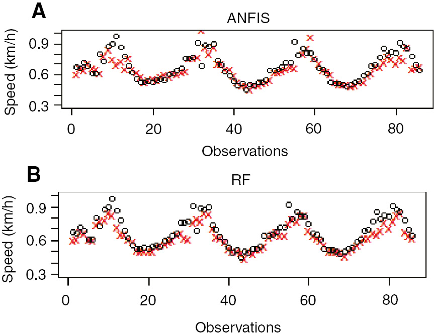
(A) Speed Prediction for the Next Hour using ANFIS. (B) RF at Site-4.

Given these results, it is worth pointing out that RF was an adequate model to predict the trigger speed for a VAS, in terms of computational performance (shorter calculation time) and efficiency (lower RMSE).

6 Conclusion and Future Work

This study has investigated a data-driven model to predict the appropriate speed of VAS. The achieved results confirmed the hypotheses that the type of vehicle and the time of the day have an effect on driver mean speed and standard deviation. SOMs were employed to explore the data and partition the input space into four clusters. An automatic trigger speed model based on historical traffic speed data was investigated to predict the trigger speed of VAS. Finally, a comparative study between RF and ANFIS was conducted to predict an appropriate speed for each cluster obtained by SOM.

From the hypotheses under test, the results suggest that the trigger speed of VAS cannot be static and that the trigger speed must be altered depending on the type of vehicle and its location, i.e. site. A differential trigger speed of VAS should be considered when there is a difference in mean speed and standard deviation between the types of vehicle. It is clear that a safe trigger speed for trucks and heavy trucks are not thoroughly considered in practice, particularly when the trigger speed is based on the 85th percentile. The mean speed of heavy trucks is often lower than the mean speed of cars, which is usually the major class (in terms of traffic volume) in the traffic stream. Ignoring this particular issue might mean a failure to give the right warning in the right time to the right type of vehicle. The RF model was found to be an appropriate model to predict the 85th percentile speed to be able to report its usage as the trigger speed of VAS. The model was trained on data collected at four different sites in Sweden to be able to verify and validate whether data-driven models based on real data can be used to predict trigger speeds or not. Further testing is therefore required and suggested before claiming applicability in real time. The fact that the investigation does not reflect safe driving habits or unanticipated and unusual road/traffic conditions further limits its applicability.

At this stage, it is worth mentioning that local traffic regulations on road segments, sign installation, and safety requirements, and so on, have not made it feasible to test the model in reality. One recommendation for the future is to carry out a before-and-after (sign installation) effect analysis to be able to gain insight into the safety effects of mean speeds of different vehicle classes. In this context, the results could be validated by triggering the sign with the 85th percentile of cars, trucks, and heavy trucks, and study the effectiveness of these various trigger speeds in mean speed and standard deviation of the speed. Another interesting idea is to embed the sign with two radars and a data logger such that the first radar can determine the appropriate trigger speed by collecting the traffic data at a certain distance, at least 100 m before the sign. The other radar can detect the speed of vehicle at a shorter distance and compare to the appropriate trigger speed. When activating the sign for a particular class of vehicle, it should be a clear message to the driver about the recommended safe speed and to which type of vehicle the recommended speed is targeted.

Acknowledgments

The authors thank SafeX for the generous help in collecting the data, particularly in radar maintenance and sign movement from one site to another. Our thanks are also extended to Westcotex for the valuable technical support for server communication with the radar and data logger, the Borlänge authority for allowing us to change test sites, and Vectura for providing radars for the experiment. Finally, we thank Intelligent Transport System, ITS Dalarna, for supporting this research.

Bibliography

[1] L. Breiman, Random forests, Mach. Learn. 45 (2001), 5–32.10.1023/A:1010933404324Search in Google Scholar

[2] L. Breiman, J. H. Friedman, R. A. Olshen and C. J. Stone, Classification and Regression Trees, Wadsworth Statistical Press, Belmont, 1984.Search in Google Scholar

[3] W. Cheng, X. Ji, C. Han and J. Xi, The mining method of the road traffic illegal data based on rough sets and association rules, ICICTA, in: Proceedings of the 2010 International Conference on Intelligent Computation Technology and Automation, vol. 3, pp. 856–859, Washington, DC, USA, 2010.10.1109/ICICTA.2010.803Search in Google Scholar

[4] Y. C. Chiou, L. W. Lan and C. M. Tseng, A novel method to predict traffic features based on rolling self-structured traffic patterns, J. Intell. Transport. Syst. 18 (2014), 352–366.10.1080/15472450.2013.806764Search in Google Scholar

[5] P. Dalgaard, Introductory Statistics with R (Statistics and Computing), Springer, New York, 2008.10.1007/978-0-387-79054-1Search in Google Scholar

[6] C. Duncan, A. Khattak and F. M. Council, Applying the ordered probit model to injury severity in truck-passenger car rear-end collisions, Transportation Research Record 1635, Transportation Research Board, National Research Council, Washington, DC, 1998.10.3141/1635-09Search in Google Scholar

[7] M. Freedman and A. F. Williams, Speeds associated with 55 mi/h and 65 mi/h speed limits in northeastern States, ITE J. 2 (1992), 17–21.Search in Google Scholar

[8] N. J. Garber and A. A. Ehrhart, Effects of speed, flow, and geometric characteristics on crash frequency for two-lane highways, Transport. Res. Rec. 1717 (2000), 76–83.10.3141/1717-10Search in Google Scholar

[9] N. J. Garber, J. S. Miller, B. Yuan and X. Sun, Safety effects of differential speed limits on rural interstate highways, Transport. Res. Rec. J. Transport. Res. Board 1 (2005), 56–62.10.3141/1830-08Search in Google Scholar

[10] A. H. Ghods, F. Saccomanno and G. Guido, Effect of car/truck differential speed limits on two-lane highways safety operation using microscopic simulation, Proc. Soc. Behav. Sci. 53 (2012), 833–840.10.1016/j.sbspro.2012.09.932Search in Google Scholar

[11] J. W. Hall and L. V. Dickinson, An Operational Evaluation of Truck Speeds on Interstate Highways, Department of Civil Engineering, University of Maryland, 1974.Search in Google Scholar

[12] D. L. Harkey and R. Mera, Safety Impacts of Different Speed Limits on Cars and Trucks, vol. FHWA-RD, pp. 93–161, U.S. Department of Transportation, Federal Highway Administration, Washington, DC, 1994.Search in Google Scholar

[13] D. W. Harwood, Highway/Heavy Vehicle Interaction, vol. 3, Transportation Research Board, 2003.Search in Google Scholar

[14] Idaho Transportation Department Planning Division, Evaluation of the Impacts of Reducing Truck Speeds on Interstate Highways in Idaho, National Institute for Advanced Transportation Technology, University of Idaho, 2002.Search in Google Scholar

[15] G. James, D. Witten, T. Hastie and R. Tibshirani, An Introduction to Statistical Learning, Springer, New York, 2013.10.1007/978-1-4614-7138-7Search in Google Scholar

[16] J. S. R. Jang, ANFIS: adaptive-network-based fuzzy inference system, IEEE Trans. Syst. Man Cybern. 23 (1993), 665–685.10.1109/21.256541Search in Google Scholar

[17] J. S. R. Jang and C. T. Sun, Neuro-fuzzy modelling and control. Proc. IEEE 83 (1995), 378–406.10.1109/5.364486Search in Google Scholar

[18] D. Jomaa, S. Yella and M. Dougherty, Automatic trigger speed for vehicle activated signs using adaptive neuro fuzzy system and classification regression trees, in: The Tenth International Multi-conference on Computing in the Global Information Technology, Malta, 2015.Search in Google Scholar

[19] D. Jomaa, M. Dougherty, S. Yella and K. Edvardsson, Effectiveness of vehicle activated signs on mean speed and standard deviation of vehicle speed, J. Transport. Safety Security 8 (2016), 293–309.10.1080/19439962.2014.976690Search in Google Scholar

[20] T. Kohonen, Self-organized formation of topologically correct feature maps, Biol. Cybernet. 43 (1982), 50–69.10.1007/BF00337288Search in Google Scholar

[21] T. McMurtry, M. Saito, M. Riffkin and S. Heath, Variable speed limits signs: effects on speed and speed variation in work zones, Transport. Res. Circ. Mainten. Manage. E-C135 (2009), 159–174.Search in Google Scholar

[22] B. Park, Hybrid neuro-fuzzy application in short-term freeway traffic volume forecasting, Transport. Res. Rec. J. Transport. Res. Board 1802 (2002), 190–196.10.3141/1802-21Search in Google Scholar

[23] P. Rämä and R. Kulmala, Effects of variable message signs for slippery road conditions on driving speed and headways, Transport. Res. F Traffic Psychol. Behav. 3 (2000), 85–94.10.1016/S1369-8478(00)00018-8Search in Google Scholar

[24] S. K. Shukla, S. Rungta and L. K. Sharma, Self-organizing map based clustering approach for trajectory data, Int. J. Comput. Trends Technol. 3 (2012), 321–324.Search in Google Scholar

[25] S. Smulders, Control of freeway traffic flow by variable speed signs, Transport. Res. B 24 (1990), 111–132.10.1016/0191-2615(90)90023-RSearch in Google Scholar

[26] S. Smulders and D. E. Helleman, Variable speed control: state-of-the-art and synthesis, in: Proceedings on Road Transport Information and Control, vol. 454, pp. 155–159, IEEE, 1998.10.1049/cp:19980174Search in Google Scholar

[27] M. Van Der Voort, M. Dougherty and S. Watson, Combining Kohonen maps with ARIMA time series models to forecast traffic flow, Transport. Res. C 4 (1996), 307–318.10.1016/S0968-090X(97)82903-8Search in Google Scholar

[28] M. J. Watts and S. P. Worner, Estimating the risk of insect species invasion: Kohonen self-organising maps versus k-means, Ecol. Modell. 220 (2009), 821–829.10.1016/j.ecolmodel.2008.12.016Search in Google Scholar

Received: 2016-12-07

Published Online: 2018-11-16

This work is licensed under the Creative Commons Attribution 4.0 Public License.

Articles in the same Issue

https://doi.org/10.1515/jisys-2016-0329

Keywords for this article

Vehicle-activated signs; adaptive neuro-fuzzy inference systems; random forest; self-organising maps; trigger speed

Creative Commons

BY 4.0