Analytic approximate solutions to the chemically reactive solute transfer problem with partial slip in the flow of a viscous fluid over an exponentially stretching sheet with suction/blowing
-
Remus-Daniel Ene
 ,
Ilare Bordeaşu
,
Ilare Bordeaşu

Abstract
This paper analytically investigates the flow as well as the chemically reactive solute transfer problem in a viscous fluid. The motion equations are reduced to a nonlinear ordinary differential equations system using the similarity transformations. The obtained nonlinear differential system is for the first time approximately solved by means of the Optimal Homotopy Asymptotic Method (OHAM). The effects of the partial slip and suction/blowing parameters are analytically analyzed. Some examples are given; the obtained results provides us with a good agreement with the numerical results and reveal that our procedure is effective, accurate and easy to use.
1 Introduction
In all hydraulic machines, the liquid fluids have chemical reactions with the materials from control structures and adjuster devices. Beyond the viscous flow, with all its implications on the energy transfer, the chemical reaction of the liquid fluid affects this transfer in a negative sense. Therefore, the establishment of some relations for the viscous flow, taking into account the chemical reaction, allows for the energetic evaluation of the flow, as more appropriate to each situation.
Hydraulic system liquids are used primarily to transmit and distribute forces to various units to be actuated. Liquids are able to do this because they are almost incompressible. Pascal’s Law states that pressure applied to any part of a confined liquid is transmitted with undiminished intensity to every other part. Manufacturers of hydraulic devices usually specify the type of liquid best suited for use with their equipment in view of the working conditions, the service required, temperatures expected inside and outside the systems, the pressures the liquid must withstand, the possibilities of corrosion, and other conditions that must be considered. If incompressibility and fluidity were the only qualities required, any liquid that is not too thick could be used in a hydraulic system. One of the most important properties of any hydraulic fluid is its viscosity. Viscosity is internal resistance to flow. A liquid such as gasoline that has a low viscosity flows easily, while a liquid such as tar that has a high viscosity flows slowly. Regardless of its function and design, every hydraulic system has a minimum number of basic components, in addition to a conduit through which the fluid is transmitted. A basic system consists of a pump, reservoir, directional valve, check valve, pressure relieve valve, selector valve, actuator, and filter [1].
In the last few decades, several researchers have studied boundary layer flow, with its practical applications in engineering, electrochemistry and polymer processing technology. Lomen et al. [2] applied a perturbation method to the transport equation for a single reactive chemical with nonlinear (quadratic) rate loss relevant to a soil and water system.
Nomenclature.
| Symbols | Names |
|---|---|
| u, v | Velocity components (m/s) |
| x, y | Cartesian coordinates (m) |
| ν | Fluid kinematic viscosity (m2/s) |
| C | Concentration of the chemically reactive species |
| C∞ | Concentration far away from the sheet |
| D | Brownian diffusion coefficient (m2/s) (Molecular diffusivity of the chemically reactive species) |
| k | Chemical reaction parameter (Variable rate of chemical conversion of the first-order irreversible reaction) |
| U | Stretching velocity (m/s) |
| Cw | Concentration on the sheet |
| U0, C0 | Reference velocity and reference concentration |
| N | Velocity slip factor |
| Sc | Schmidt number |
| β | Reaction rate parameter |
| λ | Velocity slip parameter |
| NG | Dimensionless entropy number |
| Re | Reynolds number |
| Br | Brinkman number |
| T∞ | Environmental temperature (K) |
| χ, λ1 | Dimensionless constant parameters |
| Q | Dimensionless temperature difference |
Several researchers applied the shooting method to study the asymptotic behavior of the nonlinear ordinary differential equations that describe the distribution of a solute undergoing a chemical reaction, such as: Zhao et al. [3], Bhattacharyya and Layek [4], Bhattacharyya [5], and Mukhopadhyay [6, 7, 8, 9, 10].
An approximate solution to a differential equation in the form of an analytic expression can be found by the method of series, the method of small parameters, the method of successive approximations, the perturbation method, the Ritz and Galerkin method, among others. Each of these methods defines one or more infinite processes that under certain conditions can be used to obtain an exact solution to a problem. Termination of the process after a finite number of steps yields an approximate solution. In fact, an analytical method gives a solution in the form of symbols, i.e. closed form solution. A numerical method gives solution at certain points only. Hence, the analytical solution denotes an exact solution that can be used to study the behavior of the system with varying properties.
In the last years, two interesting methods to obtain an approximate analytical solution were used for solving more sophisticated PDEs. The Homotopy Analysis Method (HAM) was developed by Liao [11] who utilized the idea of homotopy in topology. The Optimal Homotopy Asymptotic Method (OHAM) was introduced by Marinca and Herisanu [12]. An advantage of OHAM is that it does not need to identify the ħ– curve, and the control and adjustment of the convergence region is provided in a conventional way. Furthermore, the OHAM has a built in convergence criteria similar to HAM but with a greater degree of flexibility.
Along with the analytical methods, some computational methods to solve nonlinear problems from engineering and computer sciences have been developed by Li et al. [17, 18, 19, 20, 21, 22, 23, 24], Guo et al. [25], Korda et al. [26].
In this paper, the optimal homotopy asymptotic method (OHAM) [12, 13, 14, 15, 16] is applied to obtain accurate, effective analytic approximate solutions. The quality of the approximate solutions is investigated using two important statistical tests: the Bartlett test and the Durbin-Wattson test. Our procedure does not depend upon small or large parameters, and provides us with a simple way to optimally control the convergence of the approximate solutions.
2 Equations of motion
We analyze the two-dimensional flow of an incompressible viscous fluid past a flat sheet in the half-plane y > 0. As in [9], two equal and opposite forces are applied along the x- and y- axis so that the wall is stretched keeping the origin fixed. The schematic diagram of the physical model is presented in Fig. 1. Also, the continuity, momentum and concentration equations governing such a type of the flow are given as [9]:
where

Schematic diagram of the physical model.
The physical initial/boundary conditions for this case are similar as in [9], [27, 28]:
where U = U0ex/L, Cw = C∞ + C0ex/(2L), N = N1e- x/(2L) is the velocity slip factor, which changes with x (at N = 0, no-slip case is observed), N1 is the initial value of the velocity slip factor, V(x) > 0 is the velocity of suction, V(x) < 0 is the velocity of blowing, V(x) = V0ex/(2L) is the velocity on the wall, V0 is the initial strength of suction, and k0 is a constant having the same dimension as k.
Using the similarity transformations:
and substituting Eq. (4) into Eqs. (1) and (2), the governing equations become:
where Sc = ν/D and β = k0L/U0.
The initial/boundary conditions Eq. (3) become:
where
Remark
In Mukhopadhyay et al. [9] there is a major error in the Equation of concentration. By a simple computation the correct equation of concentration is Eq. (6), rather than
as in Mukhopadhyay et al. [9]. Therefore, in our paper the equation of concentration Eq. (6) is correct.
3 Basic ideas of the optimal homotopy asymptotic method
In Marinca and Herisanu [12], the optimal homotopy asymptotic method is employed to compute analytical approximate solutions for equations of the general form:
subject to the boundary / initial conditions of the type
For the flow of viscous fluid determined by Eqs. (5) and (6) with initial/boundary conditions (7), the corresponding operators L, N and B will be introduced in the next section.
Using the principle of OHAM [12, 13, 14, 15, 16], we are going to construct the following homotopy:
where p ∈ [0, 1] is the embedding parameter, L is a linear operator, and H(y, Ci) ≠ 0 is an auxiliary convergence-control function. H is a function of the variable y and of the parameters C1, C2, …, Cs.
The homotopy (10) satisfies the following properties:
If the function F has the expression:
by substituting this expression in the homotopy Eq. (10) we obtain the following relation:
If we choose the following particular expression of the operator 𝓗:
we can obtain the governing equations of F0(y) and F1(y, Ci) by equating the coefficients of p0 and p1, respectively:
F0(y) can be readily found by solving the linear Eq. (16). In order to compute F1(y, Ci) by Eq. (17), we take into account the fact that the nonlinear operator N has the general form:
where n is a positive integer, and hi(y) and gi(y) are known functions that depend on F0(y) and on N.
The general solution of the nonhomogeneous linear equation (17) is obtained by summing the general solution of the corresponding homogeneous equation and a particular solution of the nonhomogeneous equation. Unfortunately, the computation of such a particular solution is not possible in most cases, so the computation of the function F1(y, Ci), introduced as a third modified version of Optimal Homotopy Asymptotic Method in [12], consists of the following steps:
We consider the F1(y, Ci) of the form:
or
The above expressions of Hi(y, hj(y), Cj) contain linear combinations of the functions hj, j = 1, …, s. They also contain the parameters Cj, j = 1, …, s. The summation limit m is an arbitrary positive integer number.
Finally, the convergence-control parameters C1, C2, …, Cs can be optimally computed by means of various methods, such as: the least square method, the Galerkin method, the collocation method, the Kantorowich method, or the weighted residual method.
With these parameters known, the first-order approximate solution (21) is well-determined.
4 Application of the OHAM to the chemically reactive solute transfer problem
Now we are going to apply our procedure to obtain approximate solutions of Eqs. (5) and (6) with the initial / boundary conditions Eq. (7).
For this purpose, in the case of the nonlinear equation Eq. (5), we choose the linear operator of the form:
where K is an unknown positive parameter and will be determined later.
As in Marinca and Herisanu [12], it is easy to show that the linear operator is not unique.
The initial approximation f0(η) can be obtained from the following problem:
which has the solution
The nonlinear operator Nf(η), corresponding to nonlinear differential Eq. (5), is defined by:
For the initial approximation f0(η) given by Eq. (24), the nonlinear operator Eq. (25) becomes:
Comparing Eqs. (26) and (18), one can write:
The function f1(η) given by Eq. (19) becomes:
where we have freedom to choose a lot of possibilities for the unknown functions Hi, i = 1, 2, as follows (see Marinca and Herisanu [12]):
Substituting Eq. (29) into Eq. (28) we have:
where
The first-order approximate solution given by Eq. (21) is obtained from Eqs. (24) and (30):
In this way, we can find other solutions as well.
For Eq. (6) with initial/boundary condition given by Eq. (7) (for the unknown function φ), the expression for the linear operator Lφ(η) is chosen as:
where K1 > 0 is an unknown parameter at this moment.
Eq. (16) can be written in the form:
and has the solution
The nonlinear operator Nφ corresponding to the unknown function φ is obtained from the expression Eq. (6) in the form:
For the initial approximation φ0(η) given by Eq. (34), the nonlinear operator Eq. (35) becomes:
By comparing the Eqs. (18) and (36) one can get:
The first approximation φ1(η, Di), given by Eq. (19), becomes:
where Di are unknown parameters, and the unknown auxiliary functions
where
Substituting Eq. (39) into Eq. (38) one can get:
The first-order approximate solution given by Eq. (21) is obtained from Eqs. (34) and (40):
5 Results and discussions
In order to prove the accuracy of the obtained results, we will determine the convergence-control parameters K, Ci, K1 and Di, which appear in Eqs. (31) and (41), by the least square means method. In this way, the convergence-control parameters are optimally determined, and the first-order approximate solutions become known for different values of the known parameters S, λ, β and Sc. In what follows, we illustrate the accuracy of the OHAM, comparing previously obtained approximate solutions with the numerical integration results, computed by means of the shooting method combined with fourth-order Runge-Kutta method using Wolfram Mathematica 6.0 software. For some values of the parameters S, λ, β and Sc we are going to determine the approximate solutions.
Example 5.1
For the first case, we consider S = -0.5, λ = 0.1. For Eq. (31), following the procedure described above, the first-order approximate solution is obtained:
Now, in this case we give the four approximate solutions φ̄(η) for concentration obtained from Eq. (41), for different value of the Schmidt parameter Sc:
a1) the reaction rate parameter β = 0.1, the Schmidt parameter Sc = 0.7.
More results are given in Appendix 6.
Remarks
The errors between the numerical solution and the approximate solution are not natural errors, but errors derived from observations. If the errors come just from the computer approximation of the real numbers, then we can call them real errors; otherwise, they are residual errors, and some statistical tests are necessary to check if these errors hedge or hide some others terms (functions). Then, the obtained approximate solution is not the best solution. For this reason, two statistical tests are usually used: the test of homoscedasticity and the test of autocorrelation. We compute the Durbin-Wattson test for autocorrelation, and the Bartlett test for homoscedasticity:
For approximate solutions (Eq. (31)), in the case S = 0 the errors pass both tests, in the other cases (S = 1 or S = -1) some small positive autocorrelations are obtained. This behavior can be explained by the greater values of the β coefficient of rate reaction, which is difficult to be cached by a numerical solution but is rigorously included in an approximate solution.
The approximate solution should have the simplest form; i.e. should have an optimal number of parameters. A good criteria to find the optimal numbers of parameters is that given by Akaike [29] (in 1974). Given a collection of models for the dates, Akaike Informational Criterion (AIC) estimates the quality of each model, relative to each of the other models. For the least squares estimation, the AIC value of the model is the following:
where RSS = residual sum of errors, k- the number of parameters, n- the number of observations. The best model is that which finds the minimum value of AIC(k).
In our case, we compute the value of AIC for k = 12, 14, 16 parameters and find the minimum value for k = 12.
Tables 2 - 4 show the comparisons between the OHAM approximate solutions (f̄OHAM, f̄′OHAM) given by Eqs. (42), (49), (50), and numerical integration, for λ = 0.1 and different values of the suction/blowing coefficient S. Table 5 provides a comparison between the OHAM approximate solutions φ̄OHAM (concentration) given by Eqs. (43), (46), (47) and (48) for the flow with blowing, i.e. S = -0.5, and numerical results for λ = 0.1, β = 0.1 and different values of the Schmidt coefficient Sc.
Comparison between OHAM results (f, f′) given by Eq. (42) and numerical results, for S = –0.5, λ = 0.1 (relative errors: ϵf = |fnumerical − fOHAM|, ϵf′ 0 = |f′numerical − f′OHAM|)
| η | fnumerical | fOHAM given by Eq. (42) | ϵf | f′numerical | fOHAM from Eq. (42) | ϵf′ |
|---|---|---|---|---|---|---|
| 0 | -0.5 | -0.5 | 0 | 0.9077773126 | 0.9077773227 | 1.01 ⋅ 10–8 |
| 4/5 | 0.0074909817 | 0.0074077629 | 8.32 ⋅ 10−5 | 0.4327638766 | 0.4327294709 | 3.44 ⋅ 10−5 |
| 8/5 | 0.2611017466 | 0.2611117146 | 9.96 ⋅ 10−6 | 0.2266414650 | 0.2268106116 | 1.69 ⋅ 10−4 |
| 12/5 | 0.3966238195 | 0.3966963649 | 7.25 ⋅ 10−5 | 0.1228892931 | 0.1228628361 | 2.64 ⋅ 10−5 |
| 16/5 | 0.4696414089 | 0.4696460798 | 4.67 ⋅ 10−6 | 0.0648025592 | 0.0646955746 | 1.06 ⋅ 10−4 |
| 20/5 | 0.5063210253 | 0.5062657176 | 5.53 ⋅ 10−5 | 0.0296392786 | 0.0296092095 | 3.006 ⋅ 10−5 |
| 24/5 | 0.5204156378 | 0.5203725140 | 4.31 ⋅ 10−5 | 0.0072024341 | 0.0072543060 | 5.18 ⋅ 10−5 |
| 28/5 | 0.5198883866 | 0.5198975191 | 9.13 ⋅ 10−6 | -0.0074991548 | -0.0074318639 | 6.72 ⋅ 10−5 |
| 32/5 | 0.5097627316 | 0.5098134397 | 5.07 ⋅ 10−5 | -0.0171195125 | -0.0170879834 | 3.15 ⋅ 10−5 |
| 36/5 | 0.4934363158 | 0.4934931771 | 5.68 ⋅ 10−5 | -0.0232005067 | -0.0232154713 | 1.49 ⋅ 10−5 |
| 40/5 | 0.4733209745 | 0.4733525235 | 3.15 ⋅ 10−5 | -0.0267255573 | -0.0267697975 | 4.42 ⋅ 10−5 |
Comparison between OHAM results (f, f′) given by Eq. (49) and numerical results, for S = 0, λ = 0.1 (relative errors: ϵf = |fnumerical − fOHAM|, ϵf′ = |f′numerical − f′OHAM|)
| η | fnumerical | fOHAM given by Eq. (49) | ϵf | f′numerical | f′OHAM from Eq. (49) | ϵf′ |
|---|---|---|---|---|---|---|
| 0 | 0 | 0 | 0 | 0.8920112191 | 0.8920112291 | 1.00 ⋅ 10−8 |
| 4/5 | 0.4673897518 | 0.4673537169 | 3.60 ⋅ 10−5 | 0.3670253355 | 0.3670394113 | 1.40 ⋅ 10−5 |
| 8/5 | 0.6695649982 | 0.6695830109 | 1.80 ⋅ 10−5 | 0.1672482217 | 0.1673093023 | 6.10 ⋅ 10−5 |
| 12/5 | 0.7640237918 | 0.7640465048 | 2.27 ⋅ 10−5 | 0.0801628206 | 0.0801224649 | 4.03 ⋅ 10−5 |
| 16/5 | 0.8098725930 | 0.8098550411 | 1.75 ⋅ 10−5 | 0.0394093404 | 0.0393649182 | 4.44 ⋅ 10−5 |
| 20/5 | 0.8325566117 | 0.8325209434 | 3.56 ⋅ 10−5 | 0.0196234072 | 0.0196233607 | 4.64 ⋅ 10−6 |
| 24/5 | 0.8438882353 | 0.8438656573 | 2.25 ⋅ 10−5 | 0.0098344018 | 0.0098622420 | 2.78 ⋅ 10−5 |
| 28/5 | 0.8495763831 | 0.8495777875 | 1.40 ⋅ 10−6 | 0.0049446204 | 0.0049730441 | 2.84 ⋅ 10−5 |
| 32/5 | 0.8524386621 | 0.8524577684 | 1.91 ⋅ 10−5 | 0.0024901777 | 0.0025048868 | 1.47 ⋅ 10−5 |
| 36/5 | 0.8538807397 | 0.8539053805 | 2.46 ⋅ 10−5 | 0.0012551227 | 0.0012547545 | 3.68 ⋅ 10−7 |
| 40/5 | 0.8546077411 | 0.8546276346 | 1.98 ⋅ 10−5 | 0.0006328835 | 0.0006224246 | 1.04 ⋅ 10−5 |
Comparison between OHAM results (f, f′) given by Eq. (50) and numerical results, for S = 0.5, λ = 0.1 (relative errors: ϵf = |fnumerical − fOHAM|, ϵf′ 0 = |f′numerical − f′OHAM|)
| η | fnumerical | fOHAM given by Eq. (50) | ϵf | f′numerical | fOHAM from Eq. (50) | ϵf′ |
|---|---|---|---|---|---|---|
| 0 | 0.5 | 0.5 | 0 | 0.8688355156 | 0.8688355206 | 4.96 ⋅ 10−9 |
| 4/5 | 0.9053218753 | 0.9053254228 | 3.54 ⋅ 10−6 | 0.2582388571 | 0.2583911834 | 1.52 ⋅ 10−4 |
| 8/5 | 1.0103156474 | 1.0103053782 | 1.02 ⋅ 10−5 | 0.0365073971 | 0.0363862320 | 1.21 ⋅ 10−4 |
| 12/5 | 0.9961189516 | 0.9960895510 | 2.94 ⋅ 10−5 | -0.0590709734 | -0.0589898768 | 8.10 ⋅ 10−5 |
| 16/5 | 0.9304509566 | 0.9304955172 | 4.45 ⋅ 10−5 | -0.0985676220 | -0.0985102893 | 5.73 ⋅ 10−5 |
| 20/5 | 0.8461894701 | 0.8462286423 | 3.91 ⋅ 10−5 | -0.1085349302 | -0.1085936980 | 5.87 ⋅ 10−5 |
| 24/5 | 0.7609466483 | 0.7609297394 | 1.69 ⋅ 10−5 | -0.1027674406 | -0.1028300572 | 6.26 ⋅ 10−5 |
| 28/5 | 0.6836993747 | 0.6836553875 | 4.39 ⋅ 10−5 | -0.0896263299 | -0.0896290671 | 2.73 ⋅ 10−6 |
| 32/5 | 0.6181395908 | 0.6181131443 | 2.64 ⋅ 10−5 | -0.0741793261 | -0.0741391579 | 4.01 ⋅ 10−5 |
| 36/5 | 0.5648641651 | 0.5648736781 | 9.51 ⋅ 10−6 | -0.0592394367 | -0.0591955250 | 4.39 ⋅ 10−5 |
| 40/5 | 0.5228604069 | 0.5228977468 | 3.73 ⋅ 10−5 | -0.0461306368 | -0.0461071944 | 2.34 ⋅ 10−5 |
Comparison between the approximate solutions φ given by Eqs. (43), (46), (47), (48) and numerical results for λ = 0.1, S = – 0.5, β = 0.1 and different values of the Schmidt parameter Sc (relative errors: ϵφ = |φnumerical – φOHAM|)
| Sc = 0.7 | Sc = 2 | Sc = 3 | Sc = 10 | |
|---|---|---|---|---|
| η | φnumerical | φnumerical | φnumerical | φnumerical |
| 0 | 1 | 1 | 1 | 1 |
| 7/10 | 0.6563309653 | 0.4811705634 | 0.4133356959 | 0.2407707922 |
| 7/5 | 0.4413426637 | 0.2217337394 | 0.1525057373 | 0.0288952290 |
| 21/10 | 0.3013144063 | 0.0982608275 | 0.0509589853 | 0.0017932391 |
| 14/5 | 0.2081737030 | 0.0424443546 | 0.0158971840 | 0.0000668552 |
| 7/2 | 0.1453929006 | 0.0181266146 | 0.0047700395 | 3.7073158658 ⋅ 10−6 |
| 21/5 | 0.1026272704 | 0.0077469672 | 0.0014107659 | 4.8504497218 ⋅ 10−7 |
| 49/10 | 0.0732049286 | 0.0033449264 | 0.0004190735 | -2.3227934713 ⋅ 10−6 |
| 28/5 | 0.0527572988 | 0.0014693029 | 0.0001267826 | 1.1093472718 ⋅ 10−6 |
| 63/10 | 0.0383982655 | 0.0006597352 | 0.0000394466 | 2.4540273639 ⋅ 10−6 |
| 7 | 0.0282077046 | 0.0003036887 | 0.0000127039 | -5.2390950688 ⋅ 10−8 |
| η | φOHAM given by Eq. (43) | φOHAM given by Eq. (46) | φOHAM given by Eq. (47) | φOHAM given by Eq. (48) |
| 0 | 1 | 1 | 1 | 1 |
| 7/10 | 0.6563234894 | 0.4811687367 | 0.4133697770 | 0.2407413591 |
| 7/5 | 0.4413508444 | 0.2217397226 | 0.1524582990 | 0.0290780437 |
| 21/10 | 0.3013056724 | 0.0982524310 | 0.0510094743 | 0.0015675514 |
| 14/5 | 0.2081583194 | 0.0424480615 | 0.0159244709 | 0.0001859219 |
| 7/2 | 0.1453900629 | 0.0181339184 | 0.0047225861 | 0.0001553578 |
| 21/5 | 0.1026386818 | 0.0077446788 | 0.0013713877 | -0.0000195483 |
| 49/10 | 0.0732206957 | 0.0033377499 | 0.0004241938 | -0.0001091419 |
| 28/5 | 0.0527674614 | 0.0014651713 | 0.0001581552 | -0.0000923121 |
| 63/10 | 0.0383983366 | 0.0006609783 | 0.0000683943 | -0.0000307619 |
| 7 | 0.0281986506 | 0.0003081183 | 0.0000230022 | 0.0000280374 |
| η | ϵφ for Eq. (43) | ϵφ for Eq. (46) | ϵφ for Eq. (47) | ϵφ for Eq. (48) |
| 0 | 0 | 0 | 0 | 0 |
| 7/10 | 7.47 ⋅ 10−6 | 1.82 ⋅ 10−6 | 3.40 ⋅ 10−5 | 2.94 ⋅ 10−5 |
| 7/5 | 8.18 ⋅ 10−6 | 5.98 ⋅ 10−6 | 4.74 ⋅ 10−5 | 1.82 ⋅ 10−4 |
| 21/10 | 8.73 ⋅ 10−6 | 8.39 ⋅ 10−6 | 5.04 ⋅ 10−5 | 2.25 ⋅ 10−4 |
| 14/5 | 1.53 ⋅ 10−5 | 3.70 ⋅ 10−6 | 2.72 ⋅ 10−5 | 1.19 ⋅ 10−4 |
| 7/2 | 2.83 ⋅ 10−6 | 7.30 ⋅ 10−6 | 4.74 ⋅ 10−5 | 1.51 ⋅ 10−4 |
| 21/5 | 1.14 ⋅ 10−5 | 2.28 ⋅ 10−6 | 3.93 ⋅ 10−5 | 2.003 ⋅ 10−5 |
| 49/10 | 1.57 ⋅ 10−5 | 7.17 ⋅ 10−6 | 5.12 ⋅ 10−6 | 1.06 ⋅ 10−4 |
| 28/5 | 1.01 ⋅ 10−5 | 4.13 ⋅ 10−6 | 3.13 ⋅ 10−5 | 9.34 ⋅ 10−5 |
| 63/10 | 7.10 ⋅ 10−8 | 1.24 ⋅ 10−6 | 2.89 ⋅ 10−5 | 3.32 ⋅ 10−5 |
| 7 | 9.05 ⋅ 10−6 | 4.42 ⋅ 10−6 | 1.02 ⋅ 10−5 | 2.80 ⋅ 10−5 |
On the other hand, in Tables 6 and 7 the comparisons between the skin-friction coefficient f″(0) and the limit value f(∞), respectively, are presented, obtained from Eqs. (42), (49) and (50) and numerical results, for λ = 0.1 and different values of the suction/blowing coefficient S.
Comparison between the skin-friction coeffcient f″ (0) obtained by means of the OHAM and numerical results, for λ = 0.1 and different values of the suction/blowing parameter S (relative errors:
| S | ϵf″(0) | ||
|---|---|---|---|
| -0.5 | -0.9222268732 | -0.9222267721 | 1.01 ⋅ 10−7 |
| -0.3 | -0.9808736678 | -0.9808736578 | 1.00 ⋅ 10−8 |
| 0 | -1.0798878084 | -1.0798877084 | 1.00 ⋅ 10−7 |
| 0.3 | -1.1913158524 | -1.1913157524 | 9.99 ⋅ 10−8 |
| 0.5 | -1.3116448434 | -1.3116447938 | 4.96 ⋅ 10−8 |
Comparison between the limit value f (∞) obtained by means of the OHAM and numerical results, for λ = 0.1 and different values of the suction/blowing parameter S (relative errors: ϵf(∞) = |fnumerical(∞) – fOHAM(∞)|)
| S | fnumerical(∞) | fOHAM(∞) | ϵf(∞) |
|---|---|---|---|
| -0.5 | 0.2032088541 | 0.2032088596 | 5.54 ⋅ 10−9 |
| -0.3 | 0.6960935296 | 0.6960938006 | 2.71 ⋅ 10−7 |
| 0 | 0.8553478033 | 0.8553480468 | 2.43 ⋅ 10−7 |
| 0.3 | 1.0339634884 | 1.0339644067 | 9.18 ⋅ 10−7 |
| 0.5 | 0.3951795612 | 0.3951796613 | 1.00 ⋅ 10−7 |
A comparison between the mass transfer coefficient φ′(0) obtained from Eqs. (43), (46), (47) and (48) with numerical results, for the flow with blowing (S = -0.5), and for the flow with suction (S = 0.5), respectively, are presented in Tables 8 and 9, respectively.
Comparison between the mass transfer coeffcient φ′(0) obtained by means of the OHAM and numerical results, for S = –0.5, λ = 0.1 and different values of the Schmidt coeffcient Sc (relative errors:
| Sc | ϵφ′(0) | ||
|---|---|---|---|
| 0.7 | -0.6273507907 | -0.6273506907 | 1.00 ⋅ 10−7 |
| 2 | -1.0206863072 | -1.0206862840 | 2.31 ⋅ 10−8 |
| 3 | -1.1891244067 | -1.1891243967 | 1.00 ⋅ 10−8 |
| 10 | -1.6436491544 | -1.6436491442 | 1.02 ⋅ 10−8 |
Comparison between the mass transfer coeffcient φ′(0) obtained by means of the OHAM and numerical results, for S = 0.5, λ = 0.1 and different values of the Schmidt coeffcient Sc (relative errors:
| Sc | ϵφ′(0) | ||
|---|---|---|---|
| 0.7 | -0.9028032434 | -0.9028031434 | 9.99 ⋅ 10−8 |
| 2 | -2.0537968062 | -2.0537967962 | 1.00 ⋅ 10−8 |
| 3 | -2.7842989909 | -2.7842989809 | 9.99 ⋅ 10−9 |
| 10 | -7.0577817249 | -7.0577816249 | 9.99 ⋅ 10−8 |
If the analytical approximate solutions f̄ and φ̄ are given by the Eqs. (31) and (41) respectively, then the residuals from Eqs. (5) and (6) respectively are:
and
An error analysis by computing the integral of the square residuals given by Eqs. (44) and (45) is presented in Table 10.
Integral of the square residual given by Eqs. (44) and (45) respectively, for different values of the parameters S, λ, β and Sc
| S | λ | β | Sc | ||
|---|---|---|---|---|---|
| -0.5 | 0.1 | 0.1 | 0.7 | 8.08 ⋅ 10−6 | 7.94 ⋅ 10−8 |
| -0.5 | 0.1 | 0.1 | 2 | 1.25 ⋅ 10−5 | |
| -0.5 | 0.1 | 0.1 | 3 | 1.45 ⋅ 10−4 | |
| -0.5 | 0.1 | 0.3 | 0.7 | 2.46 ⋅ 10−6 | |
| -0.5 | 0.1 | 1 | 0.7 | 9.04 ⋅ 10−4 | |
| 0.5 | 0.1 | 0.1 | 0.7 | 4.03 ⋅ 10−5 | 2.44 ⋅ 10−6 |
| 0.5 | 0.1 | 0.1 | 2 | 3.15 ⋅ 10−5 | |
| 0.5 | 0.1 | 0.1 | 3 | 1.24 ⋅ 10−5 | |
The profiles of the stream function f̄(η) given by Eqs. (42), (49), (50) are depicted in Fig. 1 for λ = 0.1. We observe that the stream function f̄(η) increases with an increase of the suction/blowing coefficient S.
From Fig. 3 the velocity profiles f̄′(η) decreases with an increasing of the suction/blowing coefficient S.
Fig. 4 presents the variation of the shear-stress function f̄″(η) obtained from Eqs. (42), (48) and (50). It is noticed that the shear-stress function is increasing against an increase of the suction/blowing coefficient.
On the other hand, in Fig. 5 the profiles of the concentration function φ̄(η) for the flow with blowing (S = -0.5) and suction (S = 0.5) are plotted. It is noticed that the concentration function is decreasing with respect to an increase of the Schmidt coefficient Sc. For fixed value of the slip parameter λ and the reaction rate parameter β, from Fig. 5 we can notice that the concentration function φ̄(η) decreases against an increase of the suction/blowing coefficient S, for all the values of the Schmidt coefficient Sc.
The effect of the slip parameter λ on the chemically reactive solute flow is presented in Fig. 6 for stream function f̄(η), Fig. 7 for horizontal velocity f̄′(η) and Fig. 8 for shear-stress f̄″(η). Thus, for the flow with blowing / suction, the stream function f̄(η) and horizontal velocity f̄′(η) decrease with an increase of the slip parameter λ. Hence, we conclude that the shear-stress function f̄″(η) increases with an increase of the slip parameter λ, for all the values of the suction/blowing parameter S.
Also, from Fig. 9 we can notice that the variation of the concentration φ̄(η) decreases with the increasing of the reaction rate parameter β.
From the Tables 2 - 10 and Figs. 2 - 9 we can summarize that the approximate solutions obtained by means of the OHAM technique are effective and very accurate. This comparisons proved the accuracy, validity and flexibility of the Optimal Homotopy Asymptotic Method.

Variation of the stream function f̄(η) with increasing of the suction/blowing parameter S for λ = 0.1:
— OHAM solution; • • • • • • • • numerical solution
The obtained results are in agreement with the fluid flow scenario from a hydraulic installation for different values of the characteristic quantities: U0 = 0.1 [m/s], C0 = 0.1, ν = 46 ⋅ 10-6 [m2/s] and C∞ = 0.1, respectively.

Variation of the horizontal velocity f̄′(η) with increasing of the suction/blowing parameter S for λ = 0.1:
— OHAM solution; • • • • • • • • numerical solution

Variation of the shear stress f̄″(η) with increasing of the suction/blowing parameter S for λ = 0.1: — OHAM solution; • • • • • • • • numerical solution

Variation of the concentration φ(η) with increasing of the suction/blowing parameter S for λ = 0.1:
— OHAM solution ; • • • • • • • • numerical solution ; OHAM solution (with lines and dashing lines respectively)

Variation of the stream function f̄(η) with increasing of the slip parameter λ for different values of the suction/blowing parameter S: • • • • • • • • numerical solution ; OHAM solution (with lines and dashing lines respectively)
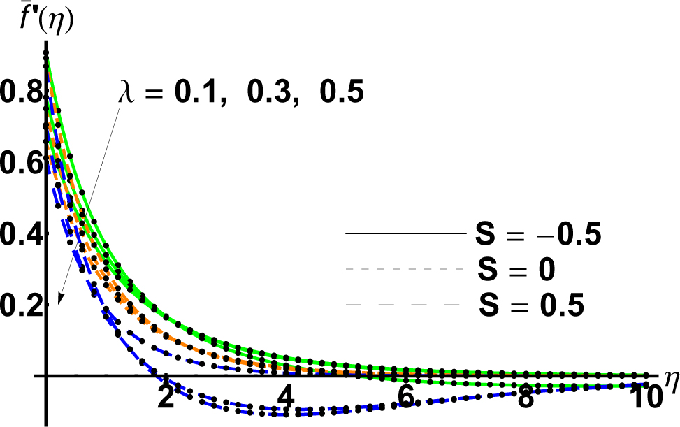
Variation of the horizontal velocity f̄′(η) with increasing of the slip parameter λ for different values of the suction/blowing parameter S: • • • • • • • • numerical solution ; OHAM solution (with lines and dashing lines respectively)

Variation of the shear stress f̄″(η) with increasing of the slip parameter λ for different values of the suction/blowing parameter S: • • • • • • • • numerical solution ; OHAM solution (with lines and dashing lines respectively)

Remarks
From Fluid Mechanics [30] it is known that the stream function decreases with respect to the increase of the slip parameter λ (this signifies the loss of energy). Following most studies in this area, there exists a correlation between the loss coefficient λ (corresponding to the slip parameter), slowing of the velocity f̄′ and the stream function f̄, with the increases of the energy losses. The obtained data in the present paper correspond to the real situation from hydraulic machines (turbines, pumps, naval propellers), where the efficiency energy of the machinery is affected by the level of turbulence.

Variation of the velocity component u from Eq. (4) for λ = 0.1, S = - 0.3, for hydraulic oil at a temperature of 40° C.

Variation of the velocity component v from Eq. (4) for λ = 0.1, S = - 0.3, for hydraulic oil at a temperature of 40° C.

The vector field (u, v) from Eq. (4) for λ = 0.1, S = - 0.3, for hydraulic oil at a temperature of 40° C.

The concentration C from Eq. (4) for λ = 0.1, S = - 0.3, Sc = 2, β = 0.1 for hydraulic oil at a temperature of 40° C.
6 Conclusions
In aerospace, hydraulic processes occur very often, with strongly nonlinear behaviors and even situations with singularities. Therefore, a numerical solution can capture all such situations and an approximate analytical solution is a more realistic option. The OHAM method does not depend upon small parameters and provides us with a convenient way to optimally control the convergence of the approximate solutions.
The analytical treatment related to the chemically reactive solute transfer problem with partial slip in the flow of a viscous fluid over an exponentially stretching sheet with suction/blowing is presented. The governing nonlinear partial differential equations (for the mass transfer and concentration) are reduced to nonlinear ordinary differential equations using some similarity transformations. The obtained nonlinear ordinary differential equations are analytically solved using the OHAM method. Some numerical examples are given for different values of the suction/blowing coefficient S. In the case of the flow with blowing (S < 0) and suction (S > 0), the effects of the Schmidt parameter Sc on the concentration φ(η) are studied. The quality of the approximate solutions are made by means of the two important statistical tests: the Bartlett test and the Durbin-Wattson test. Also, the Akaike Informational Criterion (AIC) is used to make an optimal expression of the analytical solution (from our best knowledge, this tool was not used for this reason) and this simplifies the form of the solution, being easiest in physical applications.
The obtained analytical results are compared with the corresponding numerical results obtained using the fourth-order explicit Runge-Kutta method in comparison with the shooting method. The validity, flexibility, accuracy and convergence of the approximate solutions are demonstrated by means of the auxiliary functions Hk(η, Ci) and
These comparisons proved that the OHAM technique is effective and practical.
Conflict of interest
Conflict of interests: The authors declare that there is no conflict of interests regarding the publication of this paper.
References
[1] Aviation Maintenance Technician Handbook-Airframe (FAA-H-8083-31) United States Department of Transportation, Federal Aviation Administration, Airman Testing Standards Branch, AFS-630, P.O. Box 25082, Oklahoma City, OK 73125.Search in Google Scholar
[2] Lomen D. O., Islas A. L., Fan X., Warrick A. W., A perturbation solution for nonlinear solute transport in porous media, Transport Porous Med., 1991, 6, 739–744.10.1007/978-94-017-2199-8_14Search in Google Scholar
[3] Zhao C., Hobbs B. E., Ord A., Theoretical analyses of the effects of solute dispersion on chemical-dissolution front instability in fluid-saturated porous media, Transport Porous Med., 2010, 84, 629–653.10.1007/s11242-010-9528-5Search in Google Scholar
[4] Bhattacharyya K., Layek G. C., Magnetohydrodynamic slip flow and diffusion of a reactive solute past a permeable flat plate with suction/injection, Front. Chem. Sci. Eng., 2011, 5(4), 471–476.10.1007/s11705-011-1130-zSearch in Google Scholar
[5] Bhattacharyya K., Reactive solute transfer in a stagnation-point flow over a shrinking sheet with a diffusive mass flux, J. Appl. Mech. Tech. Phy., 2015, 56(3), 464–470.10.1134/S0021894415030165Search in Google Scholar
[6] Mukhopadhyay S., Chemically reactive solute transfer in a boundary layer slip flow along a stretching cylinder, Front. Chem. Sci. Eng., 2011, 5(3), 385–391.10.1007/s11705-011-1101-4Search in Google Scholar
[7] Mukhopadhyay S., Vajravelu K., Diffusion of chemically reactive species in Casson fluid flow over an unsteady permeable stretching surface, J. Hydrodyn., 2013, 25(4), 591–598.10.1016/S1001-6058(11)60400-XSearch in Google Scholar
[8] Mukhopadhyay S., Vajravelu K., van Gorder R. A., Chemically reactive solute transfer in a moving fluid over a moving surface, Acta Mech., 2013, 224, 513–523.10.1007/s00707-012-0764-3Search in Google Scholar
[9] Mukhopadhyay S., Golam Arif M., Wazed Ali M., Effects of partial slip on chemically reactive solute transfer in the boundary layer flow over an exponentially stretching sheet with suction/blowing, J. Appl. Mech. Tech. Phy., 2013, 54(6), 928–936.10.1134/S0021894413060084Search in Google Scholar
[10] Mukhopadhyay S., Chemically reactive solute transfer in boundary layer flow along a stretching cylinder in porous medium, Afr. Mat., 2014, 25, 1–10.10.1007/s13370-012-0094-6Search in Google Scholar
[11] Liao S., Beyond Perturbation: Introduction to the Homotopy Analysis Method, Chapman and Hall, 2003.Search in Google Scholar
[12] Marinca V., Herisanu N., The Optimal Homotopy Asymptotic Method - Engineering Applications, Springer Verlag, Heidelberg, 2015.10.1007/978-3-319-15374-2Search in Google Scholar
[13] Marinca V., Ene R.-D., Marinca B., Negrea R., Different approximations to the solution of upper-convected Maxwell fluid over a porous stretching plate, Abstr. Appl. Anal., 2014, Article ID 139314, 13 pages.10.1155/2014/139314Search in Google Scholar
[14] Ene R.-D., Marinca V., Approximate solutions for steady boundary layer MHD viscous flow and radiative heat transfer over an exponentially porous stretching sheet, Appl. Math. Comput., 2015, 269, 389–401.10.1016/j.amc.2015.07.038Search in Google Scholar
[15] Ene R.-D., Szabo M. A., Danoiu S., Viscous flow and heat transfer over a permeable shrinking sheet with partial slip, Mater. Plast., 2015, 52(3), 408–412.Search in Google Scholar
[16] Marinca V., Ene R.-D., Dual approximate solutions of the unsteady viscous flow over a shrinking cylinder with Optimal Homotopy Asymptotic Method, Adv. Math. Phys., 2014, Article ID 417643, 11 pages.10.1155/2014/417643Search in Google Scholar
[17] Li S., Karatzoglu A., Gentile C., Collaborative Filtering Bandits, Proceedings of the 39th International ACM SIGIR Conference on Research and Development in Information Retrieval, (SIGIR 2016, Pisa, Tuscany, Italy), 539-548.10.1145/2911451.2911548Search in Google Scholar
[18] Gentile C., Li S., et al., On Context-Dependent Clustering of Bandits, Proceedings of the 34th International Conference on Machine Learning, (ICML 2017, Sydney, Australia), J. Mach. Learn. Res., 2017, 1253-1262.Search in Google Scholar
[19] Kar P., Li S., et al., Online Optimization Methods for the Quantification Problem, Proceedings of the 22nd ACM SIGKDD International Conference on Knowledge Discovery and Data Mining, (SIGKDD 2016, San Francisco, California, US), 1625-1634.10.1145/2939672.2939832Search in Google Scholar
[20] Hao F., Park D.-S., Li S., Lee H. M., Mining λ-Maximal Cliques from a Fuzzy Graph, Advanced IT based Future Sustainable Computing, Journal of Sustainability, 2016, 8(6), 2016, pp. 553.10.3390/su8060553Search in Google Scholar
[21] Li S., The Art of Clustering Bandits, M.Sc. thesis, Universita degli Studi dell’Insubria, 2016.Search in Google Scholar
[22] Hao F., Li S., et al., An Efficient Approach to Generating Location-Sensitive Recommendations in Ad-hoc Social Network Environments, IEEE T. Serv. Comput., 2015, 99, 520-533.10.1109/TSC.2015.2401833Search in Google Scholar
[23] Gentile C., Li S., Zappella G., Online Clustering of Bandits, Proceedings of the 31st International Conference on Machine Learning, (ICML 2014, Beijing, China), J. Mach. Learn. Res., 2014, 757-765.Search in Google Scholar
[24] Li S., et al., Medicine Rating Prediction and Recommendation in Mobile Social Networks, Proceedings of the International Conference on Green and Pervasive Computing, (May 9-11, 2013, Seoul, Korea), 2013, Vol. 7861, 216-223.10.1007/978-3-642-38027-3_23Search in Google Scholar
[25] Guo H., Feng Yi, et al., Dynamic Fuzzy Logic Control of Genetic Algorithm Probabilities, Journal of Computers, 2014, 9(1), 22-27.10.4304/jcp.9.1.22-27Search in Google Scholar
[26] Korda N., Szorenyi B., Distributed Clustering of Linear Bandits in Peer to Peer Networks, Proceedings of the 33rd International Conference on Machine Learning, (ICML 2016, New York City, NY, US), J. Mach. Learn. Res., 2016, 1301-1309.Search in Google Scholar
[27] Martin M. J., Boyd I. D., Momentum and heat transfer in a laminar boundary layer with slip flow, J. Thermo. Heat Trans., 2006, 20(4), 710–719.10.2514/1.22968Search in Google Scholar
[28] Anderson H. I., Slip flow past a stretching surface, Acta Mech., 2002, 158, 121–125.10.1007/BF01463174Search in Google Scholar
[29] Akaike H., A new look at the statistical model identification, IEEE Transaction on Automatic Control, 1974, 19(6), 716–723.10.1007/978-1-4612-1694-0_16Search in Google Scholar
[30] Giles Ranald V., Theory and problems of the Hydraulics 2nd ed., Schaum’s Outline Series, McGraw Hill Book Company, 1977.Search in Google Scholar
Appendix
the reaction rate parameter β = 0.1, the Schmidt parameter Sc = 2.
the reaction rate parameter β = 0.1, the Schmidt parameter Sc = 3.
the reaction rate parameter β = 0.1, the Schmidt parameter Sc = 10.
Example 5.2
If we consider S = 0, λ = 0.1, the expression of the first-order approximate solution is:
Example 5.3
In the last case, we consider S = 0.5, λ = 0.1. For Eq. (31), the first-order approximate solution becomes:
In what follows, we present an analytical study of the effect of the partial slip parameter λ on the chemically reactive solute transfer. In this way, we give the approximate analytical solutions for the cases: S = -0.5 < 0 - flow with blowing, S = 0 and S = 0.5 > 0 - flow with suction.
Example 5.4
If we consider S = - 0.5, λ = 0.3, for Eq. (31), the first-order approximate solution becomes:
Example 5.5
In the case when S = - 0.5, λ = 0.5, the first-order approximate solution Eq. (31) becomes:
The influence of the reaction rate parameter β on the chemically reactive solute transfer is presented below. In this way we give the approximate analytical solutions for the cases: β = 0.1, β = 0.3 and β = 1, where S = -0.5, λ = 0.1 and Sc = 0.7 are fixed.
Example 5.6
In the first case, we consider S = - 0.5, λ = 0.1, Sc = 0.7 and β = 0.1. For Eq. (41), the first-order approximate solution becomes:
Example 5.7
In the second case, if S = - 0.5, λ = 0.1, Sc = 0.7 and β = 0.3, the first-order approximate solution Eq. (41) becomes:
Example 5.8
In the last case, we consider S = 0, λ = 0.1, Sc = 0.7 and β = 1. The first-order approximate solution given by Eq. (41) becomes:
This way, we can construct other accurate approximate solutions.
© 2018 Remus-Daniel Ene et al., published by De Gruyter
This work is licensed under the Creative Commons Attribution-NonCommercial-NoDerivatives 4.0 License.
Articles in the same Issue
- Regular Article
- Real-scale comparison between simple and composite raw sewage sampling
- 10.1515/eng-2018-0017
- The risks associated with falling parts of glazed facades in case of fire
- Implementation of high speed machining in thin-walled aircraft integral elements
- Evaluating structural crashworthiness and progressive failure of double hull tanker under accidental grounding: bottom raking case
- Influence of Silica (SiO2) Loading on the Thermal and Swelling Properties of Hydrogenated-Nitrile-Butadiene-Rubber/Silica (HNBR/Silica) Composites
- Statistical Variations and New Correlation Models to Predict the Mechanical Behavior and Ultimate Shear Strength of Gypsum Rock
- Analytic approximate solutions to the chemically reactive solute transfer problem with partial slip in the flow of a viscous fluid over an exponentially stretching sheet with suction/blowing
- Thermo-mechanical behavior simulation coupled with the hydrostatic-pressure-dependent grain-scale fission gas swelling calculation for a monolithic UMo fuel plate under heterogeneous neutron irradiation
- Optimal Auxiliary Functions Method for viscous flow due to a stretching surface with partial slip
- Vibrations Analysis of Rectangular Plates with Clamped Corners
- Evaluating Lean Performance of Indian Small and Medium Sized Enterprises in Automotive Sector
- FPGA–implementation of PID-controller by differential evolution optimization
- Thermal properties and morphology of polypropylene based on exfoliated graphite nanoplatelets/nanomagnesium oxide
- A computer-based renewable resource management system for a construction company
- Hygrothermal Aging of Amine Epoxy: Reversible Static and Fatigue Properties
- The selected roof covering technologies in the aspect of their life cycle costs
- Influence of insulated glass units thickness and weight reduction on their functional properties
- Structural analysis of conditions determining the selection of construction technology for structures in the centres of urban agglomerations
- Selection of the optimal solution of acoustic screens in a graphical interpretation of biplot and radar charts method
- Subsidy Risk Related to Construction Projects: Seeking Causes
- Multidimensional sensitivity study of the fuzzy risk assessment module in the life cycle of building objects
- Planning repetitive construction projects considering technological constraints
- Identification of risk investment using the risk matrix on railway facilities
- Comparison of energy parameters of a centrifugal pump with a multi-piped impeller in cooperation either with an annular channel and a spiral channel
- Influence of the contractor’s payment method on the economic effectiveness of the construction project from the contractor’s point of view
- Special Issue Automation in Finland
- Diagnostics and Identification of Injection Duration of Common Rail Diesel Injectors
- An advanced teaching scheme for integrating problem-based learning in control education
- A survey of telerobotic surface finishing
- Wireless Light-Weight IEC 61850 Based Loss of Mains Protection for Smart Grid
- Smart Adaptive Big Data Analysis with Advanced Deep Learning
- Topical Issue Desktop Grids for High Performance Computing
- A Bitslice Implementation of Anderson’s Attack on A5/1
- Efficient Redundancy Techniques in Cloud and Desktop Grid Systems using MAP/G/c-type Queues
- Templet Web: the use of volunteer computing approach in PaaS-style cloud
- Using virtualization to protect the proprietary material science applications in volunteer computing
- Parallel Processing of Images in Mobile Devices using BOINC
- “XANSONS for COD”: a new small BOINC project in crystallography
- Special Issue on Sustainable Energy, Engineering, Materials and Environment
- An experimental study on premixed CNG/H2/CO2 mixture flames
- Tidal current energy potential of Nalón river estuary assessment using a high precision flow model
- Special Spring Issue 2017
- Context Analysis of Customer Requests using a Hybrid Adaptive Neuro Fuzzy Inference System and Hidden Markov Models in the Natural Language Call Routing Problem
- Special Issue on Non-ferrous metals and minerals
- Study of strength properties of semi-finished products from economically alloyed high-strength aluminium-scandium alloys for application in automobile transport and shipbuilding
- Use of Humic Sorbent from Sapropel for Extraction of Palladium Ions from Chloride Solutions
- Topical Issue on Mathematical Modelling in Applied Sciences, II
- Numerical simulation of two-phase filtration in the near well bore zone
- Calculation of 3D Coordinates of a Point on the Basis of a Stereoscopic System
- The model of encryption algorithm based on non-positional polynomial notations and constructed on an SP-network
- A computational algorithm and the method of determining the temperature field along the length of the rod of variable cross section
- ICEUBI2017 - International Congress on Engineering-A Vision for the Future
- Use of condensed water from air conditioning systems
- Development of a 4 stroke spark ignition opposed piston engine
- Development of a Coreless Permanent Magnet Synchronous Motor for a Battery Electric Shell Eco Marathon Prototype Vehicle
- Removal of Cr, Cu and Zn from liquid effluents using the fine component of granitic residual soils
- A fuzzy reasoning approach to assess innovation risk in ecosystems
- Special Issue SEALCONF 2018
- Brush seal with thermo-regulating bimetal elements
- The CFD simulation of the flow structure in the sewage pump
- The investigation of the cavitation processes in the radial labyrinth pump
- Testing of the gaskets at liquid nitrogen and ambient temperature
- Probabilistic Approach to Determination of Dynamic Characteristics of Automatic Balancing Device
- The design method of rubber-metallic expansion joint
- The Specific Features of High-Velocity Magnetic Fluid Sealing Complexes
- Effect of contact pressure and sliding speed on the friction of polyurethane elastomer (EPUR) during sliding on steel under water wetting conditions
- Special Issue on Advance Material
- Effect of thermo-mechanical parameters on the mechanical properties of Eurofer97 steel for nuclear applications
- Failure prediction of axi-symmetric cup in deep drawing and expansion processes
- Characterization of cement composites based on recycled cellulosic waste paper fibres
- Innovative Soft Magnetic Composite Materials: Evaluation of magnetic and mechanical properties
- Statistical modelling of recrystallization and grain growth phenomena in stainless steels: effect of initial grain size distribution
- Annealing effect on microstructure and mechanical properties of Cu-Al alloy subjected to Cryo-ECAP
- Influence of heat treatment on corrosion resistance of Mg-Al-Zn alloy processed by severe plastic deformation
- The mechanical properties of OFHC copper and CuCrZr alloys after asymmetric rolling at ambient and cryogenic temperatures