An Intelligent Approach for Predicting Stock Market Movements in Emerging Markets Using Optimized Technical Indicators and Neural Networks
-
Alma Rocío Sagaceta-Mejía
 und
Julián Alberto Fresán-Figueroa
und
Julián Alberto Fresán-Figueroa

Abstract
Integrating big data analytics and machine learning algorithms has become increasingly important in the fast-changing landscape of stock market investment. The numerical findings showcase the tangible impact of our methodology on the accuracy and efficiency of stock market trend predictions. Identifying and selecting the most salient features (technical indicators) is critical in predicting the trend direction of exchange-traded funds (ETFs) in emerging markets, leveraging financial and economic indicators. Our methodology encompasses an array of statistical techniques strategically employed to identify critical technical indicators with significant implications for time series problems. We improve the efficacy of our model by performing systematic evaluations of statistical and machine learning methods across multiple sets of features or technical indicators, resulting in a more accurate trend prediction mechanism. Notably, our approach not only achieves a substantial reduction in the computational cost of the proposed neural network model by selecting only 5% of the total technical indicators for predicting ETF trends but also enhances the accuracy rate by approximately 2%.
1 Introduction
An exchange-traded fund (ETF) is a relatively recent financial innovation that provides an alternative method for indirectly investing in international equities. They are similar to conventional investment funds in which the market value is close to the value of the underlying assets and is listed on stock exchanges. This fund allows investors to implement different investment strategies incorporating diverse geographic and economic activities rather than investing in local handmade portfolios (Deville, 2008; Antoniewicz and Heinrichs, 2014).
The most popular ETFs are designed to reflect stock indices such as the S&P 500, Nasdaq, and Dow Jones. The ease of administration, lower management costs and taxes, and allowing investors to enter and exit investment positions with minimal risk are benefits of ETFs. In addition, literature shows that ETFs offer greater diversification benefits than conventional local mutual funds (Miralles-Quiros et al., 2019). In this regard, according to Hegde and McDermott (2004), the success of ETFs is due to the simplicity with which investors may benefit from portfolio diversification at lower transaction costs than stock investment portfolios.
In this work, we focus on emerging markets ETFs, which refer to countries becoming developed markets, including countries across the Asia-Pacific region and Latin America, such as Brazil, Chile, Mexico, China, and India. Emerging economies comprise countries with rapid growth, high productivity levels, increased middle-class interest, high volatility, liquidity in local debt and equity markets, and growth potential. These ETFs are attractive for investors since emerging economies tend to grow faster than their developed counterparts, as seen in how these markets have grown over the last decade (Figure 1). Our focal point is the selection of features to predict the trend of two ETFs of the emerging markets: iShares MSCI Chile ETF (ECH) and iShares MSCI Brazil ETF (EWZ), using technical and statistical analysis to later compare them against iShares Core S&P 500 ETF (IVV).
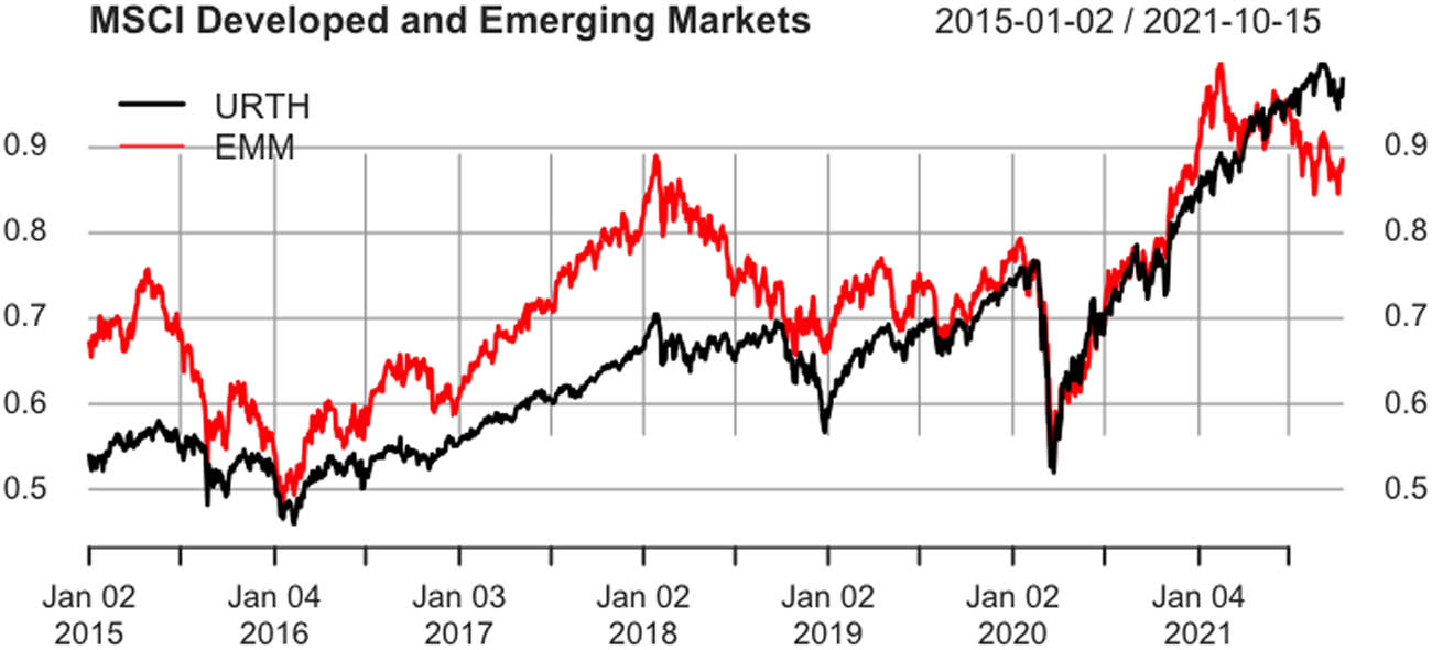
In this plot, we show the performance of two different ETFs: the iShares MSCI World ETF (Ticker: URTH), which replicates an index composed of developed market equities, and the iShares MSCI Emerging Markets ETF (Ticker: EMM), which replicates an index composed of large- and mid-capitalization emerging market equities.
Due to the energetic, nonlinear, nonparametric, and chaotic properties of stock information, stock market prediction has been a problem for analysts and researchers during the last decade. Some studies use regression methods (Chen and Chen, 2015; Jiang et al., 2020; Zhang et al., 2021) to forecast long-term stock costs or profits, while others use categorization techniques to predict patterns of stock cost development (Ananthi and Vijayakumar, 2021; Cagliero et al., 2020).
Several techniques for approaching the stock trend prediction problem have been recently developed. Initially, traditional statistical techniques were used, but with the development of artificial intelligence, machine learning algorithms helped deal with intricate market data with the development of artificial intelligence (Tang et al., 2019). A commonly used machine learning model in stock market prediction is neural networks, which have proven helpful in discovering nonlinear and nonadditive data relations, attaining superior results (De Haan et al., 2016). Even when the conventional neural network may not be the best architecture for every problem, it can successfully capture inner data relations, providing helpful information for dimensional analysis. Nevertheless, specific sorts of machine learning strategies such as restricted Boltzmann machine (RBM) (Liang et al., 2017) recurrent neural network (RNN) (Zhao et al., 2021), convolutional neural network (CNN) (Barra et al., 2020), and long short-term memory networks (LSTM) (Chen et al., 2019; Nelson et al., 2017) have shown remarkable performance in stock prediction.
Even though there have been studies to evaluate which models are more suitable for stock market prediction (Chen et al., 2021a), most of them make use of a small number of stock features, such as the highest and lowest price, opening and closing price, and some financial indicators such as the rate of change, simple moving average (SMA), exponential moving average, hull moving average, relative strength index (RSI), Williams’s indicator, or change momentum oscillator, among others. Nevertheless, there exist many indicators of stock performance (O’Hara et al., 2000).
The related literature extensively investigates several machine learning models (Fang et al., 2024; Matuozzo et al., 2023; Verma et al., 2023a,b,c). While these works have demonstrated significant advances by proposing novel model architectures, our research objectives differ from the conventional paradigm. Rather than introducing new multilayer perceptron (MLP) variants, we focus on advancing the field in an alternative way: systematically identifying salient features to improve the model’s predictive capabilities. Our innovation is based on the nuanced and meticulous selection of features, which is critical to improving computational efficiency and may increase prediction accuracy. For instance, the package Pandas Technical Analysis (Pandas TA) contains over 200 tunable technical indicators. In this article, we propose an analysis of feature selection methods based on cross-industry standard process for data mining (CRISP-DM) methodology to identify the most salient features, aiming to discriminate the best indicators, reduce the data to be processed, and assist investors in determining stock market behavior. The article has been divided as follows: in Section 2, we describe the datasets, their technical indicators, the data pre-processing, the data mining methodology, the techniques for feature selection, the artificial intelligence model, and the experiments performed; Section 3 presents the resulting subsets of features for each ETF, their cross-validated accuracy, and their percentage gain from the baseline; Section 4 discusses the results obtained in the experiments, and future research lines are presented.
2 Materials and Methods
This section describes the datasets and how they were treated before performing the experimentation. We centered our study on three datasets obtained from Yahoo Finance, calculated several technical features, and processed all the data obtained with the CRISP-DM methodology. After that, we carried out a feature analysis based on diverse techniques to identify and rank the most salient features, which were finally fed to a MLP to evaluate the performance of the selected features.
2.1 Stocks Analyzed
To reduce potential biases in the results and increase the reliability of our findings, we carefully selected a time frame for our analysis that ranged from December 12, 2009, to January 1, 2020. The rationale for this time frame is twofold. First, it allows us to exclude economic changes caused by atypical phenomena during global pandemics (Almehmadi, 2021; Verma et al., 2022), which could significantly impact the results. By focusing on the period preceding these unprecedented events, we hope to maintain the stability of our analysis and isolate the impact of other economic factors. In financial stock analysis, the utilization of pre-pandemic data assumes paramount significance, particularly concerning the introduction of innovative methodologies for indicator selection. Antecedent data are a fundamental, extensive, and stable cornerstone, facilitating the training and validation processes intrinsic to machine learning methodologies. By encompassing periods antedating the pandemic, datasets encapsulate diverse market conditions, spanning from periods of stability to instances of heightened volatility alongside various economic cycles. This diversity enables models to discern a broad spectrum of patterns and relationships within the data, augmenting their adaptability and predictive capacity. Furthermore, pre-pandemic data aids in constructing models capable of distinguishing between typical market fluctuations and extraordinary occurrences such as pandemic-induced disruptions. This differentiation is critical in averting models from succumbing to biases due to pandemic-specific irregularities, ensuring their resilience and applicability across diverse market landscapes. Thus, the incorporation of pre-pandemic data reinforces the credibility, generalizability, and effectiveness of feature selection.
In addition, our focus on BlackRock’s ETFs involved a meticulous selection of three funds: ECH, EWZ, and iShares Core S&P 500 ETF (IVV). This intentional choice represents emerging and developed markets, offering a nuanced analysis of predictive features and model performance. Enriching our analysis, we explore the sectoral distribution within each ETF, contributing to a comprehensive understanding of how different economic activities influence their performance. This sectoral consideration enhances the depth of our study, uncovering insights into the interconnectedness of sectors within emerging and developed markets and providing a more holistic view of the factors influencing ETF trends. (Table 2 for the sector distribution in this analysis.)
Table 1 shows these ETFs’ main market exposure areas, while Figure 2 depicts their Opening price during the considered period.
Market exposure of ETFs (ECH, EWZ and IVV)
| Top sectors (%) | |||||
|---|---|---|---|---|---|
| ECH | (%) | EWZ | (%) | IVV | (%) |
| Financials | 21.53 | Materials | 26.08 | Info. tech | 27.70 |
| Materials | 21.28 | Financials | 23.96 | Health care | 13.36 |
| Utilities | 18.73 | Energy | 12.83 | Cons. Disc. | 12.00 |
| Cons. Stap. | 13.92 | Cons. Stap. | 10.14 | Communication | 11.19 |
| Energy | 8.34 | Cons. Disc. | 8.44 | Financials | 10.89 |
| Total | 83.8 | Total | 81.45 | Total | 75.14 |

Behavior of Open values for ECH, EWZ, and IVV.
The data that can be obtained from Yahoo Finance for each period are the opening price Open, the highest price High, the lowest price Low, the closing price Close, the number of transactions Volume, the adjusted close price for splits, the dividends yield, and capital gain distributions Adjusted close. Table 2 presents the data summarized for the opening price.
Summarized data for the opening price Open
| ECH | EWZ | IVV | |
|---|---|---|---|
| Minimum | 29.30 | 17.49 | 103.5 |
| 1st Quartile | 40.35 | 36.69 | 137.9 |
| Median | 46.48 | 43.63 | 199.3 |
| Mean | 50.10 | 47.25 | 196.7 |
| 3rd Quartile | 59.84 | 56.30 | 244.7 |
| Maximum | 80.25 | 81.41 | 325.2 |
We use a classification strategy to predict a qualitative variable
The response variable
The
2.2 Methodological Approach Based on Data Mining
The CRISP-DM specifies the stages in which the datasets are processed (Shearer, 2000). CRISP-DM covers six stages: understanding the data and the domain of the problem, the data preparation, the construction of the model, the evaluation of the proposed model, and, finally, the presentation of the results.
Data preparation is the main stage in any data mining methodological approach. In this stage, the raw data are cleaned, merged, scaled, and feature-engineered to enhance the quality of the information, improving the machine learning algorithm’s behavior (Jamshed et al., 2019; Sun et al., 2017). The data preparation stage converts inconsistent and incomplete real-world data into a readable format. In this work, the data preparation stage was primarily based on the following activities.
2.3 Technical Indicators
This study employed the Pandas Technical Analysis Library (Pandas TA) to compute a comprehensive set of technical indicators. Pandas TA, an extension of the widely-used Pandas package, provides a versatile toolkit encompassing customizable technical indicators, utility functions, and candlestick patterns. Through the application of Pandas TA, we expanded our feature set by an additional 210 indicators from the six fundamental attributes sourced from the Yahoo Finance database, including Open, High, Low, Close, Adjusted Close, and Volume, complementing the previously acquired features. Consequently, our dataset now comprises a total of 216 daily features. This amalgamation equips our analytical framework with a rich and diverse set of features, facilitating a nuanced exploration of market trends and enhancing the depth of our predictive model.
2.4 Class Assignment
For each day
2.5 Data Normalization
Since the scales of the features computed earlier fluctuate significantly, we use a min–max approach to convert the data linearly. Every feature’s minimum values are converted to 0; afterward, the maximum values are transformed to a 1, and finally, all other values are adjusted to a decimal between 0 and 1. The formula, for each value, is given as follows:
If normalization is performed, we avoid diluting the effectiveness of an equally important feature (on a lower scale) because other features have values on a larger scale.
2.6 Data Cleaning
The process of preparing raw data for analysis by removing incomplete data is known as data cleaning, and this prepares the data for the data mining process, which needs valuable information. As in the previous step, missing or non-available data are unavoidable when technical features are calculated. For example, when calculating SMA, it is necessary to select a range of days before the day we are calculating; hence, for the initial days of the dataset, the SMA cannot be obtained; thus, the data for those will be missing. To handle this issue, we proceeded to drop each day containing unavailable data, so the database spanned from 01/01/2009 to 01/01/2020.
2.7 MLP for Predictive Analysis
An MLP was used to predict the qualitative variable
An MLP is a neural network connecting multiple neurons or perceptrons, partitioned into the input, hidden, and output layers. The nodes form a directed acyclic graph, meaning the paths connect nodes in layers from one layer to the next, as shown in Figure 4. Apart from the input ones, each neuron has a nonlinear activation function, a bias, and connecting weights, which the MLP trains by back-propagation in a supervised learning fashion (Ecer et al., 2020) so that the error value can be updated in a much more successful way. The MLP used in this work is depicted in Figure 4. We use this MLP to evaluate the performance of the different subsets of technical features obtained by several feature selection approaches described below.

The input layer cardinality of the MLP corresponds to the number of input features; there would be 216 nodes if all features are considered. The hidden layer contains (input features + classes)/2 = 109 nodes. Finally, the output layer contains only one node.
The configuration parameters for the MPL are delineated in the following excerpt:
hidden_layer_sizes = int((X.shape[1] + len(np.unique(y)))/2)
MLPClassifier(hidden_layer_sizes=hidden_layer_sizes, activation=’logistic’,
# cross-validate knn on our training sample with nof_folds=10
cv_generator = StratifiedKFold(n_splits=10, shuffle=False)
2.8 Statistical Measures for Feature Selection
As mentioned earlier, in this work, we use an approach based on exploratory analysis and reduction of the input space to improve the accuracy of multiclass classification in machine learning. This feature selection effectively reduces dimensionality, limiting the number of variables that characterize the data. This reduction is performed by selecting the subset of features that provide more information, dropping the redundant ones to obtain a significant quantity of information from a lower-dimensional space (Reddy et al., 2020). In the machine learning paradigm, a narrower input space implies a computationally efficient modeled structure since it is desirable to have input data with few variables that produce small models that generalize well. The above is especially valid for linear models with related degrees of freedom and number of inputs.
We selected features after the data cleaning and scaling stages and before the predictive model’s training phase to reduce the input space. The techniques for selecting the most relevant characteristics used in this work are described below.
2.9 Low Variance
Low variance feature removal is a basic and straightforward approach to feature selection. The low variance technique removes all characteristics whose variance does not reach the established threshold. This feature selection algorithm only works with features, not class outputs, making it an unsupervised technique. If a feature’s variance is close to zero, then a feature is approximately constant and will not improve the model’s performance. In that case, it should be removed. The expression defines the variance as follows:
where
2.10 Chi-Squared
In this method, each feature is evaluated against the classes. For each pair of features, Chi-squared values are calculated; a larger Chi-squared value commonly indicates a greater interdependence between the two attributes. This method identifies the features that are more likely to be independent of the class and thus unrelated to the classification. Since this approach is commonly used with categorical attributes, it is needed first to discretize the numeric attributes at different intervals. The next expression is used to calculate the Chi-squared statistic:
where
2.11 Least Absolute Shrinkage and Sselection Operator (LASSO)
The LASSO is a regularization technique. Regularization is one technique to address the issue of overfitting by providing new information and, as a result, modifying the model’s parameter values to induce a penalty, as can be seen in the following expressions:
where
2.12 Tree-based Feature Selection
The extra trees classifier is a meta-method that fits several randomized decision trees on various dataset subsamples and averages their results to enhance the prediction accuracy and counter over-fitting. Those randomized decision trees are extremely randomized trees created by heavily randomizing cut point and attribute selection while splitting a tree node.
2.13 Pearson’s Correlation
Pearson’s correlation coefficient calculates the linear relationship between two random variables. Its values range between
where
2.14 Principal Feature Analysis
The principal feature analysis method selects the principal features by adopting the structure of the principal components of the feature set, which retain the majority of the information, both in terms of maximum variability of the features in lower-dimensional space and minimization of the reconstruction error. This technique constructs the covariance matrix of all features and computes the eigenvectors of the matrix by applying a principal component analysis. Afterward, a vector is associated with each feature, and a
2.15 Mean Absolute Difference (MAD)
The MAD, as can be seen in equation, as the variance, is also a scaled variant. This implies that the greater the MAD, the greater the discriminating power.
where
2.16 Dispersion Ratio (DR)
For a given (positive) feature
Since
The DR can be used as a dispersion measure. When all the feature samples have (roughly) the same value, DR is close to 1, indicating a low-relevance feature. Conversely, a higher value of DR implies a higher dispersion, thus a more relevant feature (Ferreira and Figueiredo, 2012).
2.17 Cross-validation as Sampling Method
Cross-validation is a model validation approach for determining how well a model’s results generalize to a new dataset. Cross-validation aims to reduce overfitting and underfitting by defining a dataset to evaluate the model in the training phase.
This procedure splits the dataset into
| Algorithm 1 Cross-validation algorithm |
|---|
| 1: Randomly shuffle the dataset. |
| 2: Make a partition of the dataset into k groups |
| 3: for each unique group do |
| 4:
|
| 5:
|
| 6:
|
| 7: end for |
| 8: Average the model’s accuracies |
2.18 Description of the Experiment’s Methodology
The described Algorithm 2 provides a comprehensive methodology for conducting feature selection experiments and evaluating trends in ETFs. The algorithm begins with the input of raw datasets for ETFs. In the first step, feature calculation and preprocessing are executed individually for each ETF. This involves the calculation of technical indicators, class assignments, data normalization, and cleaning. Following this preprocessing, the algorithm proceeds to feature selection.
Statistical measures are used to identify salient features during the feature selection step. The algorithm, in particular, computes the first quartile of the most important features for each statistical measure and ETF. Sets of selected features are then calculated based on their appearance in at least a specified number of subsets.
Moving on to the final step, model evaluation, the algorithm employs an MLP in a
In summary, this algorithm provides a systematic and iterative approach to feature selection and evaluation that is specifically designed to identify the most salient extracted features of each ETF in the dataset.
|
Algorithm 2 The algorithm employs
|
|---|
| Input: ETF raw datasets |
| 1: for each ETF do |
| 2:
|
| 3:
|
| 4:
|
| 5:
|
| 6: end for |
| Input: Preprocessed ETF datasets |
| 7: for each ETF do |
| 8:
|
| 9:
|
| 10:
|
| 11:
|
| 12: end for |
| Input: Subsets of selected features |
|
Output:
|
| 13: for
|
| 14:
|
| 15:
|
| 16:
|
| 17:
|
| 18:
|
| 19: end for |
3 Results
The results obtained with the methodology previously described are condensed in Tables 3 and 4. Table 3 describes the results of step 11 from Algorithm 2.
Number of features selected by Algorithm 2
| Selected
|
||||||||
|---|---|---|---|---|---|---|---|---|
| ETFs | 0 | 1 | 2 | 3 | 4 | 5 | 6 | 7 |
| ECH | 216 | 101 | 72 | 39 | 20 | 10 | 4 | 0 |
| EWZ | 216 | 107 | 67 | 29 | 17 | 10 | 2 | 0 |
| IVV | 216 | 104 | 71 | 35 | 19 | 9 | 3 | 0 |
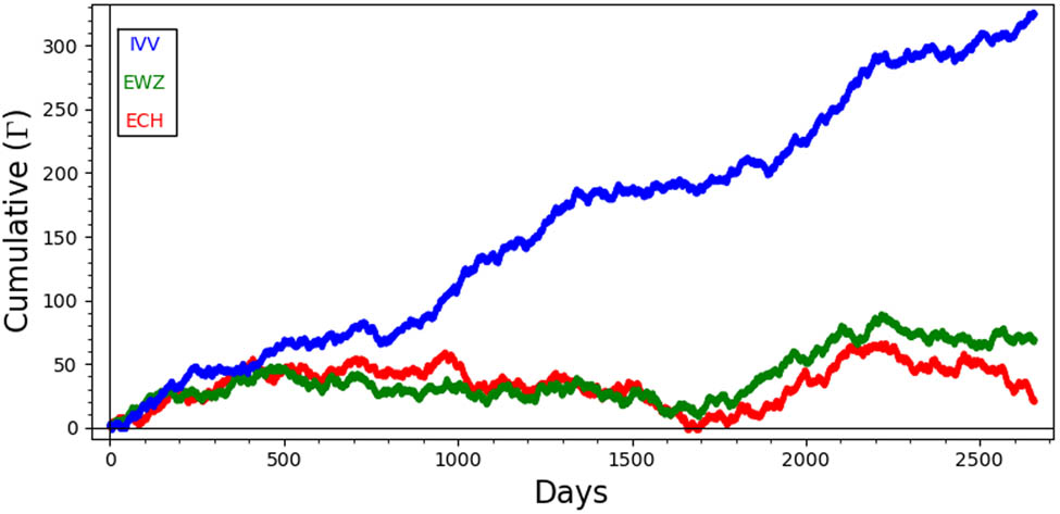
As shown in Table 4, employing the strategy described in Algorithm 2, selecting a subset of features that can provide better results using less computational resources is possible. Figure 5 shows the gain obtained by feature selection. The features in the subset Selected(5) are shown in Table 5. A brief description of these features can be found in Appendix A.
Median accuracy after cross-validation
| Accuracy (%) | |||||||
|---|---|---|---|---|---|---|---|
| ETFs | 0 | 1 | 2 | 3 | 4 | 5 | 6 |
| ECH | 78.01 | 77.82 | 78.76 | 79.33 | 80.46 | 80.27 | 59.03 |
| EWZ | 76.46 | 75.19 | 75.38 | 75.33 | 76.51 | 77.82 | 51.41 |
| IVV | 77.26 | 77.64 | 77.63 | 77.63 | 77.78 | 78.54 | 71.05 |

Percentage gain obtained by the selection of features.
Features in the respective Selected(5) sets
| ETFs | Selected(5) |
|---|---|
| ECH | AOBV_LR_2, BBP_5_2.0, BOP, CTI_12, DEC_1, EBSW_40_10, INC_1, J_9_3, K_9_3, ZS_30 |
| EWZ | AOBV_LR_2, BBP_5_2.0, BOP, CTI_12, DEC_1, EBSW_40_10, INC_1, J_9_3, STOCHk_14_3_3, WILLR_14 |
| IVV | BBP_5_2.0, BOP, DEC_1, INC_1, J_9_3, PVR, TTM_TRND_6, WILLR_14, STOCHRSIk_14_14_3_3 |
AOBV, Archer’s on balance volume; BBP, Bollinger band percent; BOP, balance of power; CTI, correlation trend indicator; DEC, decreasing; EBSW, even better SineWave; INC, increasing; STOCHRSI, stochastic relative strength index, WILLR, Williams % R.
The selected features are visually represented in Figure 6. A frequently employed metric to evaluate the similarity between sets is the Jaccard Distance. This metric offers a straightforward and intuitive approach to quantify the dissimilarity between sets, rendering it a valuable tool in diverse domains where assessing similarity or dissimilarity is important. The Jaccard Distance is defined as follows:

Venn diagram of Selected(5) features obtained for each ETF.
The Jaccard distance is a metric that is widely used in academia to measure the similarity or dissimilarity between two sets. Its range always lies between 0 and 1, where 0 signifies complete similarity (in the case of identical sets), and 1 represents complete dissimilarity (in the presence of no shared elements). Notably, the Jaccard distance is normalized, which implies that its value is independent of the size of the sets being compared, and solely depends on their relative intersection sizes and the overall set union.
In the context of studying various ETFs, it is important to consider the sets of features included in Selected(5). One key aspect of this analysis is measuring the distance between these feature sets. By examining the distance between these sets, we can gain valuable insights into the similarities and differences between various ETFs. The following distances provides a deeper understanding of the underlying characteristics of these funds:
It is apparent that ETFs pertaining to emerging markets exhibit a higher degree of proximity among themselves as compared to those that are associated with disparate markets.
We conducted further experiments, analyzing the complete set of features and the Selected(5) features for each ETF. In addition, we implemented the early stopping technique to enhance the training of the MLP model, ensuring that overfitting is avoided while improving generalization performance and optimizing computational resources. The outcomes of our tests are compiled in Table 6.
Results of the experiments using the early stopping technique
| Set | Features | Accuracy (%) | Training time (s) | Epoch |
|---|---|---|---|---|
| Full ECH | 216 | 67.01 | 41.8 | 347 |
| Select 5 ECH | 10 | 79.66 | 6.49 | 449 |
| Full EWZ | 216 | 68.32 | 45.9 | 355 |
| Select 5 EWZ | 10 | 76.28 | 6.49 | 468 |
| Full IVV | 216 | 71.10 | 53.2 | 457 |
| Select 5 IVV | 9 | 78.46 | 8.68 | 713 |
As seen in Table 6, using this standard technique, the accuracy is improved by 13.63% on average, and the training time is reduced by 84.68% on average, even when it takes more epochs to reach convergence.
3.1 Practical Implications for Investors in Emerging Markets
Our model possesses the potential to aid investors in market timing and risk management within emerging markets. Through the analysis of predictive indicators, investors can ascertain the optimal timing for entering or exiting positions in ETFs, effectively maximizing returns and minimizing losses. By comprehending market dynamics through our model, investors can promptly adjust their positions in response to changing market conditions, mitigating risks associated with market fluctuations and diminishing exposure to volatility. While our model provides valuable insights for investors operating in emerging markets, it is imperative to acknowledge its limitations and the inherent uncertainties of financial markets. Investors can optimize their investment outcomes by integrating our model into a broader investment framework and adopting a proactive and adaptable approach.
4 Conclusions and Future Directions
As a prospective avenue for future work, analyzing economic cycles presents a promising opportunity for advancing the predictive capabilities of our model. By incorporating insights into economic cycles, such as expansion, contraction, and recovery phases, investors can better understand market trend shifts, enabling them to adjust their investment strategies accordingly. By acknowledging the cyclical nature of emerging markets, investors can obtain valuable insights into potential opportunities and risks, allowing them to make informed decisions throughout the economic cycle.
Our experiments show that in each ETF analyzed, the set Selected(5) attains a better accuracy prediction, between 77.82 and 80.27%, than using the complete set of features while using only between 4.16 and 5.09% of the features. This may imply that a good selection of features can improve the efficiency of the computational resources while attaining similar or even better prediction results. Moreover, when we reduce the dimension of the dataset, we can construct a model with a reduced topology, with fewer freedom degrees and redundant features, which could reduce the training and prediction time. In high-dimensional problems, it is always important to ask ourselves whether every input is relevant and to what extent the features contribute to determining the trend the model is attaining. The methodology used in this work may help improve the prediction used by other machine learning techniques or related problems, as proposed by Chen et al. (2021b).
The indicators calculated by the Pandas-TA package (Johnson, 2021) belong to the following categories: Candles, Cycles, Momentum, Overlap, Performance, Statistics, Trend, Utility, Volatility, and Volume. The Selected(5) feature subset used for the prediction task shares similar characteristics across different ETFs. The distribution of the categories for the Selected(5) feature subset is shown in Table 7. Even though the distribution is not the same for each ETF, it is important to note that there are similarities. This may imply that the methodology proposed in this work enables the analysis of emerging markets’ and nonemerging markets’ ETFs.
Number of features selected by each ETF in accordance with the feature’s categories
| ECH | EWZ | IVV | |
|---|---|---|---|
| Cycles | 1 | 1 | 0 |
| Momentum | 4 | 5 | 4 |
| Statistics | 1 | 0 | 0 |
| Volatility | 1 | 1 | 1 |
| Volume | 1 | 1 | 1 |
| Trend | 2 | 2 | 3 |
As shown in Figure 5, there is an improving tendency of the prediction results as we approach
After analyzing the selected features for each ETF, we can observe that emerging markets depend on the cyclic behaviors of the prices while developed markets do not. We believe this is due to the market exposure of these instruments, as can be seen in Table 1. In addition, the selected feature in the volume category for the emerging markets ETFs is Archer’s on balance volume (AOBV), while on the developed market ETF is price volume rank (PVR). These features are essentially different given that PVR classifies the day according to a relation between volume and price, while AOBV provides a quantity according to a similar relation. Finally, trailing twelve months (TTM) Trend (TTM_TRND) is selected only in IVV; this supports the general idea that emerging markets’ predictions use quantitative features, while developed markets rely more on qualitative features. A brief description of the salient features can be found in Appendix A.
Herein, we center our attention on ETFs from emerging markets with similar market exposure and market value percentages; however, it is possible to choose other kinds of ETFs where the percentage of the market exposure distribution is essentially different. Furthermore, there are ETFs specialized in some sectors like energy, financial, commodities, or technology, where the performances may differ (Figure 7). We hypothesize that the selected features obtained by the algorithm proposed in this work will be similar to those other ETFs even if the market exposure, region, or topic is different, but further research is needed.
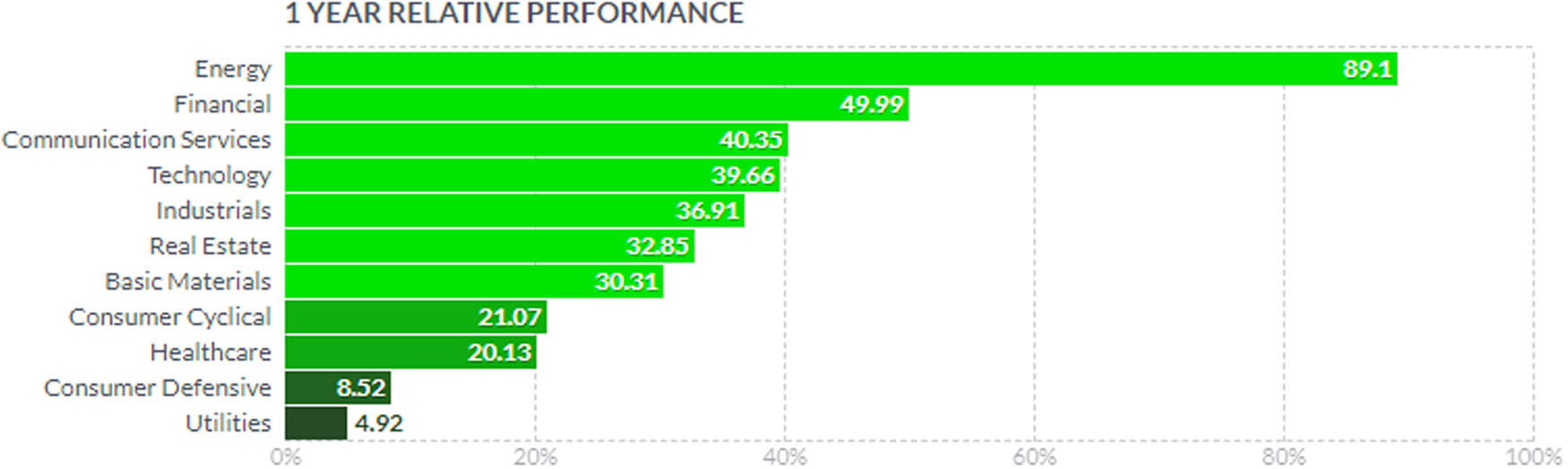
One-year growth performance per sector from 2020 to 2021, Source: October 2021. Year Relative Performance, https://finviz.com/groups.ashx.
Another interesting subject may be to determine if the methodology described in this work can provide a good selection of features that improve the performance of other neural networks models such as LSTM, RBM, RNN, and CNN, or even another techniques such as decision trees and random forest, self-organizing maps (SOM), time series, or other regression methods. Finally, this approach may be used to select features in many other interesting related topics like investment portfolios containing various stocks. It would be insightful to elaborate on an in-depth analysis of certain features that work best for emerging markets ETF’s. We believe that it depends not only on the type of market but also on the market exposure of the ETF.
Acknowledgement
This work was partially funded by the authors’ universities and the Consejo Nacional de Humanidades, Ciencias y Tecnologías (CONAHCYT) from México. Its contents are the responsibility of the authors and do not reflect the views of the research granting bodies. The authors were responsible for the data analysis after the extraction and linkage. Julián Alberto Fresán Figueroa would like to thank the support of the Universidad Autónoma Metropolitana, Unidad Cuajimalpa. Máximo Eduardo Sánchez Gutiérrez would like to thank the support of the Universidad Autónoma de la Ciudad de México, Unidad Cuautepec. Alma Rocío Sagaceta Mejía would like to thank the support of the Universidad Iberoamericana, Ciudad de México.
-
Funding information: This work has been supported by the Applied Research Institute of Technology (INIAT) of Universidad Iberoamericana, Ciudad de México.
-
Conflict of interest: Authors state no conflict of interest.
-
Article note: As part of the open assessment, reviews and the original submission are available as supplementary files on our website.
Appendix A Selected Features
In this appendix, we give a summary of the best indicators selected in our methodology. We denote by
A.1 Even Better SineWave
This indicator measures market cycles and uses a low-pass filter to remove noise. Its output is a bound signal between
A.2 Balance of Power (BOP)
BOP tells whether the underlying action in trading stock is characterized by systematic buying (accumulation) or systematic selling (distribution). The calculation of BOP is expressed as
A.3 Stochastic RSI
The Stochastic RSI technical indicator applies stochastic oscillator to the values of the RSI. The indicator thus produces two main plots, Full-
where
where
A.4 Correlation Trend Indicator
This indicator represents the correlation of the price with the trend line. The correlation is measured with the Spearman algorithm (Spearman, 1961).
A.5 KDJ
KDJ indicator is a technical indicator used to analyze and predict changes in stock trends and price patterns in a traded asset. KDJ indicator is otherwise known as the random index. It is a practical technical indicator that is most commonly used in market trend analysis of a short-term stock. The indicators are obtained as follows:
A.6 Williams % R (WILLR)
The indicator Williams % R normalizes the price as a percentage between 0 and 100. The formula is given as follows:
where Highest High corresponds to the highest high in the past
A.7 Z-score
Z-score (
A.8 Decreasing (DEC)
The indicator Decreasing computes the difference between Close values for
A.9 Increasing (INC)
Increasing is the opposite of the Decreasing indicator; it computes the difference between Close values for
A.10 TTM Trend
The TTM trend indicator colors the price bars in red or blue if the last five prices are above or under the average price for the last five price bars. Two bars of opposite colors are the signal to buy or sell.
A.11 Bollinger Bands Percent (BBP)
Bollinger band percent (
A.12 AOBV
The indicator corresponds to the average of the On Balance Volume for a given time. The formula for OBV reads as follows:
A.13 PVR
PVR compares the direction of the price change to the change in volume and assigns a number to that specific relationship. By quantifying price–volume interaction, P–V rank seeks to determine the position within a typical market cycle.
References
Almehmadi, A. (2021). Covid-19 pandemic data predict the stock market. Computer Systems Science & Engineering, 36(3), 451–460. 10.32604/csse.2021.015309Suche in Google Scholar
Ananthi, M., & Vijayakumar, K. (2021). Stock market analysis using candlestick regression and market trend prediction (CKRM). Journal of Ambient Intelligence and Humanized Computing, 12(5), 4819–4826. 10.1007/s12652-020-01892-5Suche in Google Scholar
Antoniewicz, R. S., & Heinrichs, J. (2014). Understanding exchange-traded funds: How ETFS work. Jane, Understanding Exchange-Traded Funds: How ETFs Work (September 30, 2014). 10.2139/ssrn.2523540Suche in Google Scholar
Barra, S., Carta, S. M., Corriga, A., Podda, A. S., & Recupero, D. R. (2020). Deep learning and time series-to-image encoding for financial forecasting. IEEE/CAA Journal of Automatica Sinica, 7(3), 683–692. 10.1109/JAS.2020.1003132Suche in Google Scholar
Cagliero, L., Garza, P., Attanasio, G., & Baralis, E. (2020). Training ensembles of faceted classification models for quantitative stock trading. Computing, 102, 1213–1225. 10.1007/s00607-019-00776-7Suche in Google Scholar
Chen, M.-Y., & Chen, B.-T. (2015). A hybrid fuzzy time series model based on granular computing for stock price forecasting. Information Sciences, 294, 227–241. 10.1016/j.ins.2014.09.038Suche in Google Scholar
Chen, M.-Y., Liao, C.-H., & Hsieh, R.-P. (2019). Modeling public mood and emotion: Stock market trend prediction with anticipatory computing approach. Computers in Human Behavior, 101, 402–408. 10.1016/j.chb.2019.03.021Suche in Google Scholar
Chen, W., Jiang, M., Zhang, W.-G., & Chen, Z. (2021a). A novel graph convolutional feature based convolutional neural network for stock trend prediction. Information Sciences, 556, 67–94. Suche in Google Scholar
Chen, W., Jiang, M., Zhang, W.-G., & Chen, Z. (2021b). A novel graph convolutional feature based convolutional neural network for stock trend prediction. Information Sciences, 556, 67–94. 10.1016/j.ins.2020.12.068Suche in Google Scholar
De Haan, L., Mercadier, C., & Zhou, C. (2016). Adapting extreme value statistics to financial time series: Dealing with bias and serial dependence. Finance and Stochastics, 20(2), 321–354. 10.1007/s00780-015-0287-6Suche in Google Scholar
Deville, L. (2008). Exchange traded funds: History, trading, and research. Handbook of Financial Engineering (pp. 67–98). Springer.10.1007/978-0-387-76682-9_4Suche in Google Scholar
Ecer, F., Ardabili, S., Band, S. S., & Mosavi, A. (2020). Training multilayer perceptron with genetic algorithms and particle swarm optimization for modeling stock price index prediction. Entropy, 22(11), 1239. 10.3390/e22111239Suche in Google Scholar
Ehlers, J. F. (2013). Cycle analytics for traders,+ downloadable software: Advanced technical trading concepts. John Wiley & Sons. 10.1002/9781118728611Suche in Google Scholar
Fang, W., Zhang, S., & Xu, C. (2024). Improving prediction efficiency of Chinese stock index futures intraday price by VIX-Lasso-GRU Model. Expert Systems with Applications, 238, 121968. 10.1016/j.eswa.2023.121968Suche in Google Scholar
Ferreira, A. J., & Figueiredo, M. A. (2012). Efficient feature selection filters for high-dimensional data. Pattern Recognition Letters, 33(13), 1794–1804. 10.1016/j.patrec.2012.05.019Suche in Google Scholar
Hegde, S. P., & McDermott, J. B. (2004). The market liquidity of diamonds, q’s, and their underlying stocks. Journal of Banking & Finance, 28(5), 1043–1067. 10.1016/S0378-4266(03)00043-8Suche in Google Scholar
Jamshed, H., Khan, M., Khurram, M., Inayatullah, S., & Athar, S. (2019). Data preprocessing: A preliminary step for web data mining. 3c Tecnología: Glosas de innovación aplicadas a la pyme, 8(29), 206–221. 10.17993/3ctecno.2019.specialissue2.206-221Suche in Google Scholar
Jiang, M., Jia, L., Chen, Z., & Chen, W. (2020). The two-stage machine learning ensemble models for stock price prediction by combining mode decomposition, extreme learning machine and improved harmony search algorithm. Annals of Operations Research, 309(2), 1–33. 10.1007/s10479-020-03690-wSuche in Google Scholar
Johnson, K. (2021). Pandas - technical analysis. https://github.com/twopirllc/pandas-ta. Suche in Google Scholar
Liang, Q., Rong, W., Zhang, J., Liu, J., & Xiong, Z. (2017). Restricted Boltzmann machine based stock market trend prediction. In: 2017 International Joint Conference on Neural Networks (IJCNN) (pp. 1380–1387). IEEE. 10.1109/IJCNN.2017.7966014Suche in Google Scholar
Lu, Y., Cohen, I., Zhou, X. S., & Tian, Q. (2007). Feature selection using principal feature analysis. In Proceedings of the 15th ACM International Conference on Multimedia, MM ’07 (pp. 301–304). New York, NY, USA: Association for Computing Machinery. 10.1145/1291233.1291297Suche in Google Scholar
Matuozzo, A., Yoo, P. D., & Provetti, A. (2023). A right kind of wrong: European equity market forecasting with custom feature engineering and loss functions. Expert Systems with Applications, 223, 119854. 10.1016/j.eswa.2023.119854Suche in Google Scholar
Miralles-Quirós, J. L., Miralles-Quirós, M. M., & Nogueira, J. M. (2019). Diversification benefits of using exchange-traded funds in compliance to the sustainable development goals. Business Strategy and the Environment, 28(1), 244–255. 10.1002/bse.2253Suche in Google Scholar
Nelson, D. M., Pereira, A. C., & de Oliveira, R. A. (2017). Stock market’s price movement prediction with LSTM neural networks. In 2017 International Joint Conference on Neural Networks (IJCNN) (pp. 1419–1426). IEEE. 10.1109/IJCNN.2017.7966019Suche in Google Scholar
O’Hara, H. T., Lazdowski, C., Moldovean, C., & Samuelson, S. T. (2000). Financial indicators of stock price performance. American Business Review, 18(1), 90. Suche in Google Scholar
Reddy, G. T., Reddy, M. P. K., Lakshmanna, K., Kaluri, R., Rajput, D. S., Srivastava, G., & Baker, T. (2020). Analysis of dimensionality reduction techniques on big data. IEEE Access, 8, 54776–54788. 10.1109/ACCESS.2020.2980942Suche in Google Scholar
Shearer, C. (2000). The CRISP-DM model: The new blueprint for data mining. Journal of Data Warehousing, 5(4), 13–22. Suche in Google Scholar
Spearman, C. (1961). The proof and measurement of association between two things. Appleton-Century-Crofts. 10.1037/11491-005Suche in Google Scholar
Sun, W., Cai, Z., Liu, F., Fang, S., & Wang, G. (2017). A survey of data mining technology on electronic medical records. In: 2017 IEEE 19th International Conference on e-Health Networking, Applications and Services (Healthcom) (pp. 1–6). 10.1109/HealthCom.2017.8210774Suche in Google Scholar
Tang, H., Dong, P., & Shi, Y. (2019). A new approach of integrating piecewise linear representation and weighted support vector machine for forecasting stock turning points. Applied Soft Computing, 78, 685–696. 10.1016/j.asoc.2019.02.039Suche in Google Scholar
Verma, S., Sahu, S. P., & Sahu, T. P. (2022). Stock market analysis of beauty industry during covid-19. In: Advances in Data Computing, Communication and Security: Proceedings of I3CS2021 (pp. 157–168), Springer. 10.1007/978-981-16-8403-6_14Suche in Google Scholar
Verma, S., Sahu, S. P., & Sahu, T. P. (2023a). Portfolio management using additive ratio assessment based stock selection and deep learning for prediction. International Journal of Information Technology, 15(8), 4055–4062. 10.1007/s41870-023-01493-3Suche in Google Scholar
Verma, S., Sahu, S. P., & Sahu, T. P. (2023b). Stock market forecasting with different input indicators using machine learning and deep learning techniques: A review. Engineering Letters, 31(1), 213–229. Suche in Google Scholar
Verma, S., Sahu, S. P., & Sahu, T. P. (2023c). Two-stage hybrid feature selection approach using levy’s flight based chicken swarm optimization for stock market forecasting. Computational Economics, 1–32. https://doi.org/10.1007/s10614-023-10400-8.10.1007/s10614-023-10400-8Suche in Google Scholar
Zhang, J., Li, L., & Chen, W. (2021). Predicting stock price using two-stage machine learning techniques. Computational Economics, 57(4), 1237–1261.10.1007/s10614-020-10013-5Suche in Google Scholar
Zhao, J., Zeng, D., Liang, S., Kang, H., & Liu, Q. (2021). Prediction model for stock price trend based on recurrent neural network. Journal of Ambient Intelligence and Humanized Computing, 12, 745–753. 10.1007/s12652-020-02057-0Suche in Google Scholar
© 2024 the author(s), published by De Gruyter
This work is licensed under the Creative Commons Attribution 4.0 International License.
Artikel in diesem Heft
- Regular Articles
- Political Turnover and Public Health Provision in Brazilian Municipalities
- Examining the Effects of Trade Liberalisation Using a Gravity Model Approach
- Operating Efficiency in the Capital-Intensive Semiconductor Industry: A Nonparametric Frontier Approach
- Does Health Insurance Boost Subjective Well-being? Examining the Link in China through a National Survey
- An Intelligent Approach for Predicting Stock Market Movements in Emerging Markets Using Optimized Technical Indicators and Neural Networks
- Analysis of the Effect of Digital Financial Inclusion in Promoting Inclusive Growth: Mechanism and Statistical Verification
- Effective Tax Rates and Firm Size under Turnover Tax: Evidence from a Natural Experiment on SMEs
- Re-investigating the Impact of Economic Growth, Energy Consumption, Financial Development, Institutional Quality, and Globalization on Environmental Degradation in OECD Countries
- A Compliance Return Method to Evaluate Different Approaches to Implementing Regulations: The Example of Food Hygiene Standards
- Panel Technical Efficiency of Korean Companies in the Energy Sector based on Digital Capabilities
- Time-varying Investment Dynamics in the USA
- Preferences, Institutions, and Policy Makers: The Case of the New Institutionalization of Science, Technology, and Innovation Governance in Colombia
- The Impact of Geographic Factors on Credit Risk: A Study of Chinese Commercial Banks
- The Heterogeneous Effect and Transmission Paths of Air Pollution on Housing Prices: Evidence from 30 Large- and Medium-Sized Cities in China
- Analysis of Demographic Variables Affecting Digital Citizenship in Turkey
- Green Finance, Environmental Regulations, and Green Technologies in China: Implications for Achieving Green Economic Recovery
- Coupled and Coordinated Development of Economic Growth and Green Sustainability in a Manufacturing Enterprise under the Context of Dual Carbon Goals: Carbon Peaking and Carbon Neutrality
- Revealing the New Nexus in Urban Unemployment Dynamics: The Relationship between Institutional Variables and Long-Term Unemployment in Colombia
- The Roles of the Terms of Trade and the Real Exchange Rate in the Current Account Balance
- Cleaner Production: Analysis of the Role and Path of Green Finance in Controlling Agricultural Nonpoint Source Pollution
- The Research on the Impact of Regional Trade Network Relationships on Value Chain Resilience in China’s Service Industry
- Social Support and Suicidal Ideation among Children of Cross-Border Married Couples
- Asymmetrical Monetary Relations and Involuntary Unemployment in a General Equilibrium Model
- Job Crafting among Airport Security: The Role of Organizational Support, Work Engagement and Social Courage
- Does the Adjustment of Industrial Structure Restrain the Income Gap between Urban and Rural Areas
- Optimizing Emergency Logistics Centre Locations: A Multi-Objective Robust Model
- Geopolitical Risks and Stock Market Volatility in the SAARC Region
- Trade Globalization, Overseas Investment, and Tax Revenue Growth in Sub-Saharan Africa
- Can Government Expenditure Improve the Efficiency of Institutional Elderly-Care Service? – Take Wuhan as an Example
- Media Tone and Earnings Management before the Earnings Announcement: Evidence from China
- Review Articles
- Economic Growth in the Age of Ubiquitous Threats: How Global Risks are Reshaping Growth Theory
- Efficiency Measurement in Healthcare: The Foundations, Variables, and Models – A Narrative Literature Review
- Rethinking the Theoretical Foundation of Economics I: The Multilevel Paradigm
- Financial Literacy as Part of Empowerment Education for Later Life: A Spectrum of Perspectives, Challenges and Implications for Individuals, Educators and Policymakers in the Modern Digital Economy
- Special Issue: Economic Implications of Management and Entrepreneurship - Part II
- Ethnic Entrepreneurship: A Qualitative Study on Entrepreneurial Tendency of Meskhetian Turks Living in the USA in the Context of the Interactive Model
- Bridging Brand Parity with Insights Regarding Consumer Behavior
- The Effect of Green Human Resources Management Practices on Corporate Sustainability from the Perspective of Employees
- Special Issue: Shapes of Performance Evaluation in Economics and Management Decision - Part II
- High-Quality Development of Sports Competition Performance Industry in Chengdu-Chongqing Region Based on Performance Evaluation Theory
- Analysis of Multi-Factor Dynamic Coupling and Government Intervention Level for Urbanization in China: Evidence from the Yangtze River Economic Belt
- The Impact of Environmental Regulation on Technological Innovation of Enterprises: Based on Empirical Evidences of the Implementation of Pollution Charges in China
- Environmental Social Responsibility, Local Environmental Protection Strategy, and Corporate Financial Performance – Empirical Evidence from Heavy Pollution Industry
- The Relationship Between Stock Performance and Money Supply Based on VAR Model in the Context of E-commerce
- A Novel Approach for the Assessment of Logistics Performance Index of EU Countries
- The Decision Behaviour Evaluation of Interrelationships among Personality, Transformational Leadership, Leadership Self-Efficacy, and Commitment for E-Commerce Administrative Managers
- Role of Cultural Factors on Entrepreneurship Across the Diverse Economic Stages: Insights from GEM and GLOBE Data
- Performance Evaluation of Economic Relocation Effect for Environmental Non-Governmental Organizations: Evidence from China
- Functional Analysis of English Carriers and Related Resources of Cultural Communication in Internet Media
- The Influences of Multi-Level Environmental Regulations on Firm Performance in China
- Exploring the Ethnic Cultural Integration Path of Immigrant Communities Based on Ethnic Inter-Embedding
- Analysis of a New Model of Economic Growth in Renewable Energy for Green Computing
- An Empirical Examination of Aging’s Ramifications on Large-scale Agriculture: China’s Perspective
- The Impact of Firm Digital Transformation on Environmental, Social, and Governance Performance: Evidence from China
- Accounting Comparability and Labor Productivity: Evidence from China’s A-Share Listed Firms
- An Empirical Study on the Impact of Tariff Reduction on China’s Textile Industry under the Background of RCEP
- Top Executives’ Overseas Background on Corporate Green Innovation Output: The Mediating Role of Risk Preference
- Neutrosophic Inventory Management: A Cost-Effective Approach
- Mechanism Analysis and Response of Digital Financial Inclusion to Labor Economy based on ANN and Contribution Analysis
- Asset Pricing and Portfolio Investment Management Using Machine Learning: Research Trend Analysis Using Scientometrics
- User-centric Smart City Services for People with Disabilities and the Elderly: A UN SDG Framework Approach
- Research on the Problems and Institutional Optimization Strategies of Rural Collective Economic Organization Governance
- The Impact of the Global Minimum Tax Reform on China and Its Countermeasures
- Sustainable Development of Low-Carbon Supply Chain Economy based on the Internet of Things and Environmental Responsibility
- Measurement of Higher Education Competitiveness Level and Regional Disparities in China from the Perspective of Sustainable Development
- Payment Clearing and Regional Economy Development Based on Panel Data of Sichuan Province
- Coordinated Regional Economic Development: A Study of the Relationship Between Regional Policies and Business Performance
- A Novel Perspective on Prioritizing Investment Projects under Future Uncertainty: Integrating Robustness Analysis with the Net Present Value Model
- Research on Measurement of Manufacturing Industry Chain Resilience Based on Index Contribution Model Driven by Digital Economy
- Special Issue: AEEFI 2023
- Portfolio Allocation, Risk Aversion, and Digital Literacy Among the European Elderly
- Exploring the Heterogeneous Impact of Trade Agreements on Trade: Depth Matters
- Import, Productivity, and Export Performances
- Government Expenditure, Education, and Productivity in the European Union: Effects on Economic Growth
- Replication Study
- Carbon Taxes and CO2 Emissions: A Replication of Andersson (American Economic Journal: Economic Policy, 2019)