Predicting early mortality for patients in intensive care units using machine learning and FDOSM
-
Kareem Hameed Khalaf
 and
Dhafar Hamed Abd
and
Dhafar Hamed Abd

Abstract
An accurate prediction of mortality in intensive care units (ICUs) is crucial to improving patient outcomes and optimizing resource allocation. However, existing methods often lack high-dimensional data and interpretability, rely on outdated equipment, or fail to integrate multifaceted clinical data effectively. This study aims to develop a hybrid predictive model integrating machine learning (ML), the fuzzy decision-by-opinion score method (FDOSM), and explainable artificial intelligence (XAI) to enhance the accuracy, transparency, and clinical applicability of the prediction of mortality forecasts. The dataset was used from Zigong Fourth People’s Hospital and consisted of 1,210 patients and 182 attributes. Using Chi-square feature selection, we identified statistically significant features (e.g. vital signs, lab results) from ICU patient records, reducing dimensionality while preserving predictive power. We evaluated multiple ML models (including LightGBM, Extra Trees, Support Vector Machine, K-Nearest Neighbours, XGBoost, Random Forest, and Artificial Neural Network) using a comprehensive dataset of ICU patient records, which includes vital signs, laboratory results, and clinical interventions. The FDOSM was then integrated to assess model outputs against domain-specific criteria, enabling nuanced risk stratification and enhancing decision support in critical care. XAI techniques were used to interpret the outputs of the best-performing model, improving trust in the predictions. Our hybrid approach achieved superior performance, with the Extra Tree algorithm trained on the refined feature set obtaining the highest rank 1, with a weight of 0.14375, an AUC of 88.173%, a precision of 90.244%, and an accuracy of 88.167%. The results demonstrate that combining Chi-square-driven feature selection with ML-FDOSM and XAI integration significantly improves mortality prediction, offering a reliable and transparent tool for critical care settings.
1 Introduction
Given the critical condition and limited survival time of patients in the intensive care units (ICUs), early mortality prediction is vital to saving lives [1]. The complexity of patient sequence data and dynamic treatment patterns in the ICU complicate the application of standard sequential models for mortality prediction [2]. Patients in the ICU undergo intensive monitoring through medical instruments, generating continuous and multimodality time-series medical data that are recorded, such as simple bedside monitoring data (heart rate, arterial blood pressure, etc.) and laboratory tests, which are not limited to blood sugar, blood gas chemical tests, etc. Under these conditions, the use of ML to predict mortality for patients in the ICU is meaningful and necessary [3]. ICU mortality is high and, on average, 20–50% of the patients who witness ICU stay die in hospitals [4]. A mortality prediction model has the capacity to compute the severity of each patient if adopted, so that treatment can be oriented to the severity-graded patients. The ICU plays a crucial role in the treatment of critically ill patients, where timely and accurate mortality prediction can significantly affect clinical decision-making. However, early mortality prediction remains a complex challenge due to the high-dimensional and heterogeneous nature of ICU data. Traditional prediction models often lack interpretability, making it difficult for healthcare professionals to trust and act on predictions effectively. Furthermore, feature selection is critical in refining predictive models, as redundant or irrelevant features can lead to overfitting and reduced generalization.
Consistent and real-time attention will improve the timely prediction of mortality risk before it occurs, which might prevent it by taking preemptive measures and also sourcing for another mechanism, which will enhance its introduction. Furthermore, an accurate mortality prediction mechanism can be adopted in other countries to help healthcare providers with a prioritization scheme (i.e. “pay more attention to this patient”) and also predict and send a required signal in other countries to introduce a management scheme (i.e. “this patient should be transferred to a higher-level ward). Automated patient flags can strengthen the clinical decision support system [5,6].
In recent times, research in the field of artificial intelligence (AI) techniques, especially ML, has been widely embraced and adopted in the advanced world, most especially in the area of telemedicine and healthcare informatics to assist crucial clinical tasks, exploring the potential of big data for timely and effective healthcare provision [7]. Physiological state monitoring and mortality risk prediction are considered to be the two most important applications of ML in ICUs [8].
Physicians require a comprehensive understanding of recurring patient outcomes for hospital operations, resource allocation, personnel scheduling, and decision support systems. Between 5 and 20% of the hospitalized patients die, and this fraction increases to 10–40% for patients admitted to the ICU, depending on various factors such as the underlying disease, the type of hospital, and local health care systems [9].
ML, a subfield of AI, is capable of automatically recognizing patterns and creating predictive models based on pattern recognition and the learning of an input dataset. In particular, in medical informatics, ML has shown promising results in various fields, such as medical diagnoses, cancer predictions, disease classifications, and prognostic predictions [10,11]. ML strategies can provide a more dynamic source of information while accommodating data with variable frequency and time delays. Recent trends in data mining, networking, and computer technologies allow the application of such strategies in clinical health care, which can further help this study to achieve its goal [12,13].
While many studies have successfully applied machine learning (ML) to ICU outcome prediction, challenges remain in clinical implementation and interpretability [14]. These outcome predictions have helped improve the optimization and customization of treatments to reduce medical costs [15]. Furthermore, as the amount of ICU data and the quality of AI algorithms are improving, the performance and outcomes of ML models are expected to improve. Although various ML models, such as LightGBM (LGBM) [16], Extra Trees (ET) [17], Support Vector Machine (SVM), K-Nearest Neighbours (KNN), XGBoost [18], Random Forest (RF), and Artificial Neural Network (ANN) are used for the prediction in mortality of ICU patients, a key challenge has been to demonstrate the interpretability and fairness of those models. Thus, in the field of medicine, especially for models applied to patients at greatest risk of unexpected ICU mortality, it is important not only that the transparency of these models be improved but also that they preserve their power and fairness to reduce life and death caused by misleading predictions.
To address these challenges, we propose an explainable ML framework that integrates the Chi-square for feature selection and multi-criterion decision making (MCDM). For the applied MCDM, FDOSM was applied for evaluating and selecting the best model. The chi-square test helps identify the most relevant clinical characteristics associated with early mortality, improving efficiency and interpretability. FDOSM, a decision-making approach, provides a structured evaluation of model performance across multiple criteria, ensuring robustness and reliability in ICU mortality predictions [19,20]. By incorporating these techniques, our approach improves the transparency of ML predictions, enabling clinicians to make more informed and data-driven decisions. This study comprehensively assesses multiple ML models on real ICU data sets to validate the effectiveness of the proposed method. The results show improved predictive accuracy and interpretability, providing clinicians with a reliable tool for the assessment of the risk of early mortality.
We aim to meet the needs of healthcare facilities and hospital managers, who, at any given time, require information on the future status of ICU patients and need to allocate limited resources and minimize waste effectively. Given the constraints of ICU space and the availability of intensivists, nurses often also attend to less critical patients. By focusing on a resolution time of days, this study enables longer forecasting intervals rather than immediate patient care decisions, facilitating the integration of findings from multiple forecasting studies. The main contributions of this study are as follows.
XGBoost, ANN, RF, KNN, LGBM, SVM, and ET performed a comprehensive evaluation to assess their performance in predicting mortality in the ICU using multiple evaluation metrics, including precision, precision, recall, F-score, MCC, kappa score, and AUC, to identify the most effective approaches.
Development of a hybrid ML-FDOSM framework that integrates ML models and the FDOSM approach to enhance decision-making for ICU mortality.
Applied Chi-square as a feature selection to identify the most significant predictors while employing LIME to improve model transparency and trustworthiness.
The remainder of this work is structured as follows. Section 2 discusses the Related Work, reviewing existing literature and approaches relevant to the study. Section 3 presents methodology details for the dataset, preprocessing steps, and feature selection method (Chi-Square), and presents the hybrid ML-FDOSM method with evaluation metrics. Section 4 discusses the limitations of the results and the comparative analysis. Finally, Section 5 concludes with future directions for the ICU.
2 Related work
Research on mortality prediction in the ICU has been ongoing because of its vital significance in enhancing patient outcomes and allocating resources as efficiently as possible. Although they have established a solid foundation, traditional ICU mortality prediction models, like the Simplified Acute Physiology Score (SAPS) and the Acute Physiology and Chronic Health Evaluation (APACHE), frequently have interpretability and predictive accuracy issues when used with high-dimensional and heterogeneous clinical data [21,22]. By utilizing big datasets and intricate feature sets, ML techniques have recently demonstrated promise in getting beyond these restrictions.
Deep learning (DL) and ensemble models have been widely explored for mortality prediction in ICU settings. For example, a DL model focusing on patients with paralytic ileus used SHAP analysis to identify a small subset of clinical laboratory features, achieving an AUC of 0.887 on the MIMIC-IV dataset [23]. Similarly, LightGBM and RF models applied to traumatic brain injury data demonstrated superior predictive performance compared to traditional clinical scores such as APACHE II and Sequential Organ Failure Assessment (SOFA), with area under the curve (AUC) values exceeding 0.9 [24]. These studies highlight the utility of feature selection methods combined with powerful ML algorithms to improve prediction accuracy.
Feature selection plays a critical role in mortality prediction to reduce model complexity and enhance interpretability. Nature-inspired algorithms such as particle swarm optimization (PSO) and genetic algorithms (GA) have been employed to optimize feature subsets, thereby improving model performance and transparency [25]. Furthermore, methods like SHAP and other XAI techniques have been increasingly integrated to interpret model outputs and facilitate clinical trust in automated decision support systems [23,25,26].
Numerous studies have created models for predicting mortality that are specific to particular patient groups. For instance, the CanICU model targeted critically ill cancer patients using nine easily accessible variables, achieving an AUROC of 0.94 and demonstrating robust external validation across diverse cohorts [22]. Additionally, prediction models have been created for immunocompromised patients, identifying important predictors such as blood urea nitrogen and urine output using explainability techniques and several ML algorithms [26]. ML and ensemble techniques, which use feature selection and class balance to attain better performance metrics, have also been beneficial for paediatric ICU mortality prediction [27]. The comparative summary of related work is displayed in Table 1.
Summary of widely used ICU methods for mortality prediction
| Ref | Target | Dataset | ML | Feature selection | XAI |
|---|---|---|---|---|---|
| [23] | Paralytic Ileus | MIMIC-IV | Neural Net | SHAP-based | √ |
| [21] | General ICU | SIR | RF, GB, NN, LR | Top 20 vars | × |
| [24] | TBI ICU | Chi Mei | RF, LightGBM | Manual | × |
| [22] | ICU Cancer | MIMIC + Korea | RF (CanICU) | Manual | × |
| [26] | Immunocompromised | MIMIC-IV | 10 ML | None | √ |
| [27] | Pediatric ICU | Paediatric ICU | CatBoost, RF | Embedded | × |
| [25] | Heart Failure ICU | MIMIC-III | LR, DT, GB, RF | FPA, GA, PSO | √ |
| Our work | General ICU | Zigong Hospital | 7 ML | Chi-square | √ |
Despite these developments, many current models still struggle to maintain interpretability in clinical settings and integrate complex clinical data, including vital signs, lab results, and therapies. Additionally, few studies have fully integrated ML, feature selection, and XAI to provide mortality risk assessments that are both accurate and clinically interpretable.
In order to fill these gaps, our study suggests a hybrid strategy that enhances mortality prediction in ICU patients by combining various chi-square, ML classifiers, the FDOSM, and XAI approaches. We show that adding FDOSM enables domain-specific evaluation of model outputs, improving nuanced risk categorization, using a dataset of 182 attributes from 1,210 patients at Zigong Fourth People’s Hospital. Furthermore, integrating XAI methods with the top-performing ML model enhances openness and confidence, finally providing a trustworthy and comprehensible tool for predicting ICU mortality.
3 Proposed methodology
The proposed model for the prediction of mortality in patients in the ICU combines ML and FDOSM to enhance precision and interpretability. The model operates in five phases, which are dataset, preprocessing, feature selection, ML algorithms, and evaluation of FDOSM, as shown in Figure 1.
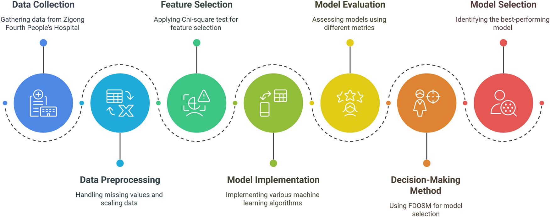
Proposed framework for patient mortality in the ICU using ML-FDOSM. The framework consists of five main stages: (1) dataset collection, (2) preprocessing of data, (3) selection using the Chi-square method, (4) training and evaluation of ML models, and (5) evaluation based on FDOSM using multiple evaluation metrics. Source: Created by the authors.
3.1 Dataset collection
The dataset used in conducting this investigation was collected from the Zigong Fourth People’s Hospital Critical Care database [28], which is publicly accessible through Physionet [29]. The dataset was collected from January 2019 to December 2020 with approval number 2021-014 from the ethics committee at Zigong Fourth People’s Hospital. The dataset consists of 1,210 patients in the ICU and patients who were infected; most were septic and/or had septic shock. The construction of such a complete database was achieved by merging high-dimensional data, such as laboratory results, baseline data, and diagnostic and geriatric nursing charts. The dataset includes 182 distinct clinical variables that cover demographic information, vital signs, laboratory results, and clinical interventions. Table 2 presents a comprehensive categorization of the dataset into five groups: demographics, vital signs, laboratory tests, ICU administration, and outcome measures. For each category, it provides the total number of columns, the number of columns with missing data, the percentage of columns with missing data, and the average percentage of missing values per column. The dataset shows massive missing data in laboratory tests, presenting a critical challenge for predictive models. Addressing this issue is crucial for ensuring the validity and reliability of ML.
Column categories and missing data
| Column category | Total columns | Columns with missing data | Columns with missing data (%) | Avg missing per column (%) |
|---|---|---|---|---|
| Demographics | 4 | 1 | 25 | 2 |
| Vital signs | 28 | 18 | 64 | 15 |
| Laboratory tests | 120 | 107 | 89 | 38 |
| ICU administration | 19 | 12 | 63 | 22 |
| Outcome measures | 11 | 4 | 36 | 8 |
| Total | 182 | 142 | 78 | 29 |
3.2 Preprocessing
In this study, we implemented several comprehensive preprocessing steps on the patient dataset from the ICU to ensure optimal data quality input for the ML models. These steps included handling missing data, scaling, encoding, and class imbalance. These steps are very important for ML to ensure that the data are clean and structured before being fed into the ML models.
Step 1: Missing values can affect the performance of ML models if not handled properly. In this study, we employed the mean technique for handling the missing values with the appropriate statistical mean. For the mean statistic, we used the numerical value.
Step 2: Scaling ensures that numerical features have a uniform range, preventing features with large values from dominating the model. In this study, the Z score is used to convert the characteristics to have a mean of 0 and a standard deviation of 1, as shown in equation (1):
Step 3: ML models cannot process categorical data directly, so encoding is necessary. In this study, One-Hot Encoding was applied to convert categorical variables into binary columns. Let us assume that we have F as a feature and k is the unique category, then
Step 4: Class imbalance occurs when one class significantly outnumbers another, leading to biased predictions of the ML model. We have two classes, survived (718) and unsurvived (492). In this study, we applied the oversampling method. The synthetic minority oversampling technique (SMOTE) is used to address this issue by generating synthetic samples for the minority class rather than simply duplicating existing ones. SMOTE creates samples using the KNN approach. The steps are (i) to randomly select a minority class instance, (ii) find its nearest neighbours k (5), and (iii) to generate synthetic instances by interpolating between the selected instance and one of its neighbours.
3.3 Feature selection
Feature selection plays an important role in the construction of the training set [30]. The entire data process is considered a feature operation. One common approach to this research in the use of ML, especially for classification tasks, is to use the Chi-square test (χ²) as a feature selection method [31]. The result of this test determines whether there is a relationship between categorical features and the target variable of interest. For each feature, this test compares the observed versus expected class frequencies, assuming the independence of classes. Equation (3) for calculating the Chi-square statistic:
where
3.4 Training and evaluation of the ML model
We evaluate multiple ML algorithms to determine the most effective model for the prediction of patient mortality in IUC. These algorithms are LGBM, ET, SVM, KNN, XGBoost, RF, and ANN. These algorithms are based on various learning mechanisms, and each algorithm brings unique advantages to a dataset and problem domain, as shown in Table 3.
Criteria for selection and comparative analysis algorithm
| Criteria | ANN | XGBoost | RF | KNN | LGBM | SVM | ET |
|---|---|---|---|---|---|---|---|
| Model complexity | High | Moderate | Moderate | Low | Moderate | High | Moderate |
| Training time | Long | Fast | Moderate | Slow | Fast | Moderate | Fast |
| Scalability | Poor | Good | Good | Poor | Good | Moderate | Good |
| Interpretability | Low | Moderate | High | High | High | Low | High |
| Handling missing data | Poor | Good | Good | Poor | Good | Poor | Good |
| Feature | High | Low | Low | Low | Low | Low | Low |
| Accuracy | High | High | Moderate | Moderate | High | High | High |
| Hyperparameter | Complex | Moderate | Simple | Simple | Simple | Moderate | Simple |
| Robustness to noise | Low | High | High | Low | High | Low | High |
| Overfitting | High | Low | Moderate | High | Low | High | Low |
| Model type | Non-linear | Non-linear | Ensemble (Bagging) | Non-linear | Ensemble (Boosting) | Non-linear (Kernel-based) | Ensemble (Bagging) |
| Suitability for large datasets | Low | High | High | Low | High | Moderate | High |
| Parallelization | Poor | Good | Good | Poor | Good | Moderate | Good |
For training ML algorithms, we can assume that we have a dataset as D = (x
i
, y
i
), where x
i
represents characteristics and y
i
represents class targets. Hypothesis function
| Algorithm 1: ML learning and evaluation |
|---|
| Input: Set of training and testing samples |
|
|
|
|
| Initialization: |
|
|
| Calculate the parameter for each algorithm |
| Learning: |
| For
|
|
|
| Testing: |
| For
|
|
| Output: |
| Learning algorithms with optimal parameters
|
Parameter setting
| Algorithm | Parameters |
|---|---|
| ANN | Hidden layer = 100, activation function = relu, solver = adam, learning rate = 0.4, Max iterations = 200, Random state = 42 |
| XGBoost | Estimators = 100, Learning rate = 0.1, Max depth = 6, Random state = 42 |
| RF | Estimators = 100, Criterion: gini, Max features = sqrt, Random state = 42 |
| KNN | K = 5, Weight function = uniform |
| LGBM | Estimators = 100, Learning rate = 0.1, Max depth = 7, Random state = 42 |
| SVM | Kernel = rbf, Regularization = 1.0, Gamma = scale |
| ET | Estimators = 100, Criterion = gini, Random state = 42 |
Size of the split dataset
| Class | Training size (70%) | Testing size (30%) | Total |
|---|---|---|---|
| Non-survival | 503 | 216 | 719 |
| Survival | 502 | 215 | 717 |
| Total | 1,005 | 431 | 1,436 |
Evaluation metrics are used to assess the performance of ML models [32,33]. These metrics provide insight into how well a model differentiates between different classes, helping in model selection and improvement.
The percentage of true outcomes among all investigated instances is measured by accuracy, as shown in equation (3). It serves as a broad gauge of how often the model is accurate.
(3)where TP represents Ture Positive, TN represents True Negative, FP represents False Positive, and FN represents False Negative.
Precision evaluates how well the model predicts positive outcomes, as shown in equation (4). It shows the proportion of positive situations that are truly positive. A low rate of false positives indicates high precision of the model.
(4)Recall gauges how well the model can accurately identify each pertinent positive case in the dataset, as shown in equation (5). It is also called sensitivity or true positive rate. It shows the proportion of real positive cases that the model can capture.
(5)The F score, also called the F1 score, is the harmonic mean of recall and precision, as shown in equation (6). This gives the measure that balances both precision and recall, which is very helpful in striking a balance between them.
(6)A statistic called Kappa is used to assess inter-rater agreement in categorical items, as shown in equation (7). It views the agreement as occurring by accident. A −1 value denotes perfect agreement, a 0 denotes agreement not better than chance, and a negative value implies agreement worse than chance.
(7)where P o is the actual agreement and P e is the predictable by chance.
The AUC is derived from the ROC curve and is computed as the area under the ROC curve, as shown in equation (8).
(8)The Matthews correlation coefficient (MCC) is a balanced measure that takes into account all four elements of the confusion matrix, as shown in equation (9):
3.5 Fuzzy evaluation framework
FDOSM is the type of MCDM method that combines fuzzy logic with expert opinions to handle subjectivity in decision making [34,35]. Subjective judgements constitute a fundamental component of FDOSM, as evident by its applicability in fields such as supplier selection, healthcare management, risk assessment, and project evaluation. Unlike traditional methods that rely on crisp numerical data, FDOSM allows decision makers to evaluate alternatives using linguistic terms such as “no difference,” “slight difference,” “difference,” etc. Then they are converted into numerical fuzzy numbers for mathematical processing. FDOSM is important in (i) expert judgments are vague and (ii) criteria have different scales. The steps for using FDOSM are the following [36]:
Step 1: Define the decision problem
This study requires a careful structuring of the decision problem prior its using FDOSM, and it should be structured. This involves three parameters: alternatives, criteria, and weights, as shown in Table 6. To identify alternatives (A 1, A 2, …, Aₙ), which are ML models in this study, we used seven models. For criteria (C 1, C 2, …, Cₘ), which are evaluation metrics such as accuracy, precision, recall, and so on. Criteria can be defined as higher is better or lower is better, which will depend on the evaluation metrics. In this study, we use higher because all evaluation metrics when higher will be better. Finally, weights (W 1, W 2, …, Wₘ) reflect the relative importance of each criterion, which can be crisp weights or fuzzy weights; in our study, we use fuzzy specific triangular.
Fuzzy decision matrix
| Alternatives/criteria | Evaluation metrics | ||||||
|---|---|---|---|---|---|---|---|
| C1 | C2 | C3 | C4 | C5 | C6 | C7 | |
| A1(ANN) | A1-C1 | A1-C2 | A1-C3 | A1-C4 | A1-C5 | A1-C6 | A1-C7 |
| A2(XGBoost) | A2-C1 | A2-C2 | A2-C3 | A2-C4 | A2-C5 | A2-C6 | A2-C7 |
| A3(RF) | A3-C1 | A3-C2 | A3-C3 | A3-C4 | A3-C5 | A3-C6 | A3-C7 |
| A4(KNN) | A4-C1 | A4-C2 | A4-C3 | A4-C4 | A4-C5 | A4-C6 | A4-C7 |
| A5(LGBM) | A5-C1 | A5-C2 | A5-C3 | A5-C4 | A5-C5 | A5-C6 | A5-C7 |
| A6(SVM) | A6-C1 | A6-C2 | A6-C3 | A6-C4 | A6-C5 | A6-C6 | A6-C7 |
| A7(ET) | A7-C1 | A7-C2 | A7-C3 | A7-C4 | A7-C5 | A7-C6 | A7-C7 |
C1 = precision, C2 = recall, C3 = F score, C4 = Kappa, C5 = AUC, C6 = MCC and C7 = accuracy. Also, the weight of each cell, such as A1-C1.
Step 2: Expert opinions
Experts evaluate each alternative using linguistic phrases, which are “No Difference,” “Slight Difference,” “Difference,” “Big Difference,” and “ Huge Difference,” because human judgment is often imprecise. These phrases are then converted to triangular fuzzy members (NFN) to handle uncertainty, as shown in Table 7. Experts can assign TFN to each alternative for each criterion.
Expert evaluation, which has three values: lower (L) possible value, middle (M) value, and upper (U) maximum possible value
| Linguistic terms | TFN (L, M, and U) | Acronyms |
|---|---|---|
| No difference | (0.00, 0.10, 0.30) | ND |
| Slight difference | (0.10, 0.30, 0.50) | SD |
| Difference | (0.30, 0.50, 0.75) | D |
| Big difference | (0.50, 0.75, 0.90) | BD |
| Huge difference | (0.75, 0.90, 1.00) | HD |
The experts could evaluate and construct the FDM, as shown in Table 5. The FDM is organized into a structured format, which is the intersection between alternatives and criteria. The cells have the fuzzy score, which has three values (L, M, and U) to become a triangle.
Step 3: Normalize the FDM
Since evaluation criteria may have different measurement scales, normalization assures fair comparison. In this study, all evaluation metrics used were higher such as accuracy, precision, recall, and so on. Then, we use equation (10):
where
L
ij
M
ij
, and
U
ij
are original fuzzy scores for alternative i under criterion j. Also,
Step 4: Fuzzy weighting
In this study, a triangular fuzzy number is used as the weight for each criterion, as shown in equation (11). Then, the normalized fuzzy scores are multiplied by the criterion weights using equation (12). The weights must approximately sum to 1 after defuzzification:
where
Step 5: Aggregate fuzzy scores
In this step, we will combine weighted fuzzy scores for each alternative using fuzzy addition shown in equation (13):
Step 6: Defuzzify the aggregated scores
In this step, we convert fuzzy scores into crisp values for ranking. In this study, we will use the centroid (C) method, as shown in equation (14):
Step 7: Rank alternatives
This is a final step that sorts (in ascending order) the alternatives based on the defuzzied score; the rank number 1 is considered the best, followed by the rank number 2, and so on.
4 Results and discussion
In this section, we conduct experiments using four groups of study subjects and objectives, followed by a comprehensive results analysis. The evaluated components comprise seven ML algorithms, Chi-square tests, FDOSM evaluation, and explainable AI techniques. Within this framework, each patient represents an instance, while the categories correspond to the baseline survived or non-survived
Prediction algorithms can be framed within the context of general or algorithmic biases, including the challenge of overfitting, which is a common issue in all learning algorithms. Ultimately, each of the learning algorithms discussed later will be applied to evaluate the results and facilitate model comparisons.
4.1 Utilization of all features in model training
In this study, all features were used during the training phase of various ML algorithms to ensure that potentially informative variables were not omitted. Utilizing the complete feature set enabled the models to capture the full dimensionality of the data, facilitating the detection of complex and non-linear relationships that could enhance predictive accuracy. This strategy proved particularly effective with robust algorithms such as ANN, ET, and XGBoost, which are designed to handle high-dimensional input spaces while managing feature importance internally. The results, as in Table 8, demonstrate that the use of all features provides a strong baseline for evaluating algorithm effectiveness and serves as a foundation for subsequent experimentation with feature selection or dimensionality reduction techniques.
Performance comparison of ML algorithms using all features
| Model | Precision | Recall | F-score | Kappa | AUC | MCC | Accuracy |
|---|---|---|---|---|---|---|---|
| ANN | 78.788 | 85.849 | 82.167 | 54.383 | 76.699 | 54.713 | 78.237 |
| XGBoost | 81.818 | 89.151 | 85.327 | 62.467 | 80.668 | 62.847 | 82.094 |
| RF | 83.111 | 88.208 | 85.584 | 63.833 | 81.521 | 64.011 | 82.645 |
| KNN | 82.87 | 84.434 | 83.645 | 60.16 | 79.965 | 60.176 | 80.716 |
| LGBM | 82.456 | 88.679 | 85.455 | 63.152 | 81.095 | 63.422 | 82.369 |
| SVM | 79.325 | 88.679 | 83.742 | 57.601 | 78.114 | 58.218 | 79.89 |
| ET | 83.929 | 88.679 | 86.239 | 65.588 | 82.419 | 65.744 | 83.471 |
Table 8 presents a compilation of several features utilized in this research, comparing seven algorithms on various metrics, including precision, recall, F-score, Kappa, AUC, MCC, and Accuracy. The overall performance of the ET model surpasses all metrics and achieves the highest F-score (86.239), Kappa (65.588), MCC (65.744), and accuracy (83.471). ET models have exhibited and guided precision while still having to maintain their balance, which makes them strong competitors for this classification task. Other metrics, such as the SVM and ANN models, demonstrate relatively weaker performance in all evaluation metrics, making them less reliable compared to other classifiers. Despite this limitation, the performance of their comparative model is commendable based on seven key metrics using the full set of features, as shown in Figure 2.
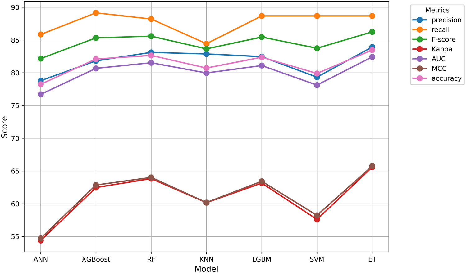
Performance comparison of ML algorithms using all features. Source: Created by the authors.
4.2 Effect of feature selection on model performance
To enhance model performance and reduce dimensionality, the chi-squared feature selection method was applied to identify and retain the most relevant input features. This statistical test measures the dependence between each feature and the target variable, assigning higher scores to features with a stronger association. During this analysis, we employed the Chi-square to choose the top 20 highlight features of the dataset, as shown in Table 9.
Most important features selected using Chi-square for model optimization
| No. | Feature | Chi-Square score |
|---|---|---|
| 1 | Sequence check | 117.66 |
| 2 | UA | 90.936 |
| 3 | CysC | 86.452 |
| 4 | Urea | 85.197 |
| 5 | BNP | 80.295 |
| 6 | PTR | 76.064 |
| 7 | Oxygen.flow.end | 73.049 |
| 8 | D2 | 72.09 |
| 9 | AST | 72.06 |
| 10 | Enzymatic method | 64.132 |
| 11 | LAC | 63.922 |
| 12 | PT | 59.004 |
| 13 | temputure_end | 58.634 |
| 14 | tn-i | 58.087 |
| 15 | INR | 52.87 |
| 16 | LDH | 52.821 |
| 17 | myo | 51.235 |
| 18 | EGFR | 46.02 |
| 19 | CK-MB | 42.52 |
| 20 | HBDH | 42.365 |
By selecting the top-ranked features based on their chi-square scores, the dataset was effectively reduced while preserving essential information. This reduction contributed to a lower computational cost and improved the generalizability of the learning algorithms. As evidenced in Table 8, the most consistently selected features exhibit a significant statistical relationship with the target variable, making them critical contributors to model performance. The general results of the evaluation, presented in Table 10, reveal that the models trained on these selected characteristics achieved competitive or improved performance compared to those trained on the full feature set. These findings confirm the effectiveness of Chi-squared feature selection in refining model input and enhancing predictive accuracy.
Features selected by Chi-squares and model performance
| Model | Precision | Recall | F-score | Kappa | AUC | MCC | Accuracy |
|---|---|---|---|---|---|---|---|
| ANN | 82.895 | 87.5 | 85.135 | 69.369 | 84.68 | 69.477 | 84.687 |
| XGBoost | 87.963 | 87.963 | 87.963 | 75.87 | 87.935 | 75.87 | 87.935 |
| RF | 87.383 | 86.574 | 86.977 | 74.014 | 87.008 | 74.018 | 87.007 |
| KNN | 89.032 | 63.889 | 74.394 | 55.945 | 77.991 | 58.328 | 77.958 |
| LGBM | 88.835 | 84.722 | 86.73 | 74.017 | 87.012 | 74.096 | 87.007 |
| SVM | 90.206 | 81.019 | 85.366 | 72.164 | 86.091 | 72.543 | 86.079 |
| ET | 90.244 | 85.648 | 87.886 | 76.337 | 88.173 | 76.436 | 88.167 |
As shown in Table 10, ET consistently demonstrates a superior performance compared to other models, making it highly appropriate for tasks with powerful classification, and its performance and balance can be a trade-off between precision and recall. Additionally, XGBoost also has strong performance, particularly in terms of recall and F1-score. This robust performance makes it particularly suitable for evaluation scenarios. On the contrary, there are some weaknesses as evidenced in the KNN performance on several metrics.
Variations in observed performance emphasized the choice of models based on specific task requirements as well as priorities for performance. This may be valid for ET, RF, and XGBoost in general terms because they have good performance. Figure 3 shows the performance metrics of seven ML models with the chi-square method, where each line represents a comparison of how models perform across different evaluation criteria.
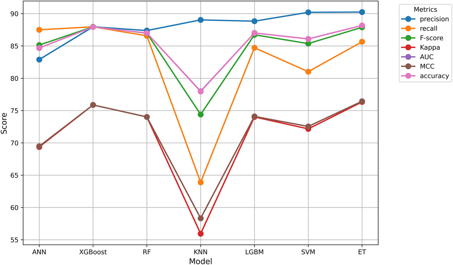
Performance comparison of various ML models using the Chi-square method. The figure illustrates the strengths and trade-offs in classification performance. Source: Created by the authors.
4.3 FDOSM
The application of FDOSM yielded significant insight into the MCDM problem under the study. In this study, the judgment of two experts was adopted, as they have approximately 8 years of experience in the field of ML classification. The first expert evaluation was adopted to evaluate all features in Table 8. The second expert’s evaluation was used to evaluate the results in Table 10. By aggregating expert opinions through linguistic variables and converting them into fuzzy numbers, the method effectively handled uncertainty and subjectivity in the evaluation process, as shown in Tables 11 and 12. The analysis revealed varying degrees of preference among the alternatives, and the defuzzification process provided crisp scores that facilitated the classification. Sensitivity analysis confirmed the robustness of the rankings, as minor variations in fuzzy membership functions did not significantly alter the optimal choice. The lowest-ranked alternative consistently outperformed others across multiple criteria, validating its suitability, as shown in Table 13.
Expert evaluation of model performance metrics without feature selection using linguistic terms
| Model | Precision | Recall | F-score | Kappa | AUC | MCC | Accuracy |
|---|---|---|---|---|---|---|---|
| ANN | D | D | D | D | D | D | D |
| XGBoost | SD | ND | ND | SD | SD | SD | SD |
| RF | ND | ND | ND | SD | SD | ND | SD |
| KNN | ND | D | SD | SD | SD | SD | D |
| LGBM | ND | ND | ND | ND | ND | ND | SD |
| SVM | ND | SD | SD | SD | SD | SD | D |
| ET | ND | ND | ND | ND | ND | ND | ND |
Expert evaluation of model performance metrics with feature selection using linguistic terms
| Model | Precision | Recall | F-score | Kappa | AUC | MCC | Accuracy |
|---|---|---|---|---|---|---|---|
| ANN | BD | ND | SD | BD | D | BD | BD |
| XGBoost | D | ND | ND | ND | ND | ND | SD |
| RF | D | ND | ND | SD | ND | SD | SD |
| KNN | SD | BD | D | HD | BD | HD | HD |
| LGBM | SD | SD | ND | SD | ND | SD | SD |
| SVM | ND | D | SD | D | SD | D | D |
| ET | ND | SD | ND | ND | ND | ND | ND |
Weight and classification of alternative results with and without feature selection
| Model | All features | Chi square | Final decision | |||
|---|---|---|---|---|---|---|
| Weight | Rank | Weight | Rank | Weight | Rank | |
| ANN | 0.5167 | 7 | 0.5417 | 6 | 0.5292 | 7 |
| XGBoost | 0.2375 | 4 | 0.2229 | 2 | 0.2302 | 3 |
| RF | 0.1958 | 3 | 0.2646 | 4 | 0.2302 | 4 |
| KNN | 0.3333 | 6 | 0.7021 | 7 | 0.5177 | 6 |
| LGBM | 0.1542 | 2 | 0.2583 | 3 | 0.20625 | 2 |
| SVM | 0.3063 | 5 | 0.3875 | 5 | 0.3469 | 5 |
| ET | 0.1333 | 1 | 0.1542 | 1 | 0.14375 | 1 |
Table 13 presents a comparative performance (weights and rankings) of different ML models in three scenarios: using all features, using Chi-square, and using a final decision that combines both all features and Chi-square. ET consistently achieved the highest ranking (1) across all three scenarios. The final decision ranks the models as the worst ANN because the rank is 7. This suggests that ensemble methods such as ET and XGBoost are strong choices, whereas ANN and KNN underperform. The results highlight that model performance depends on both the algorithm and the feature selection method, recommending ET for optimal results. Figure 4 shows that ET achieves the lowest weights, which means the best performance across all features and Chi-square.
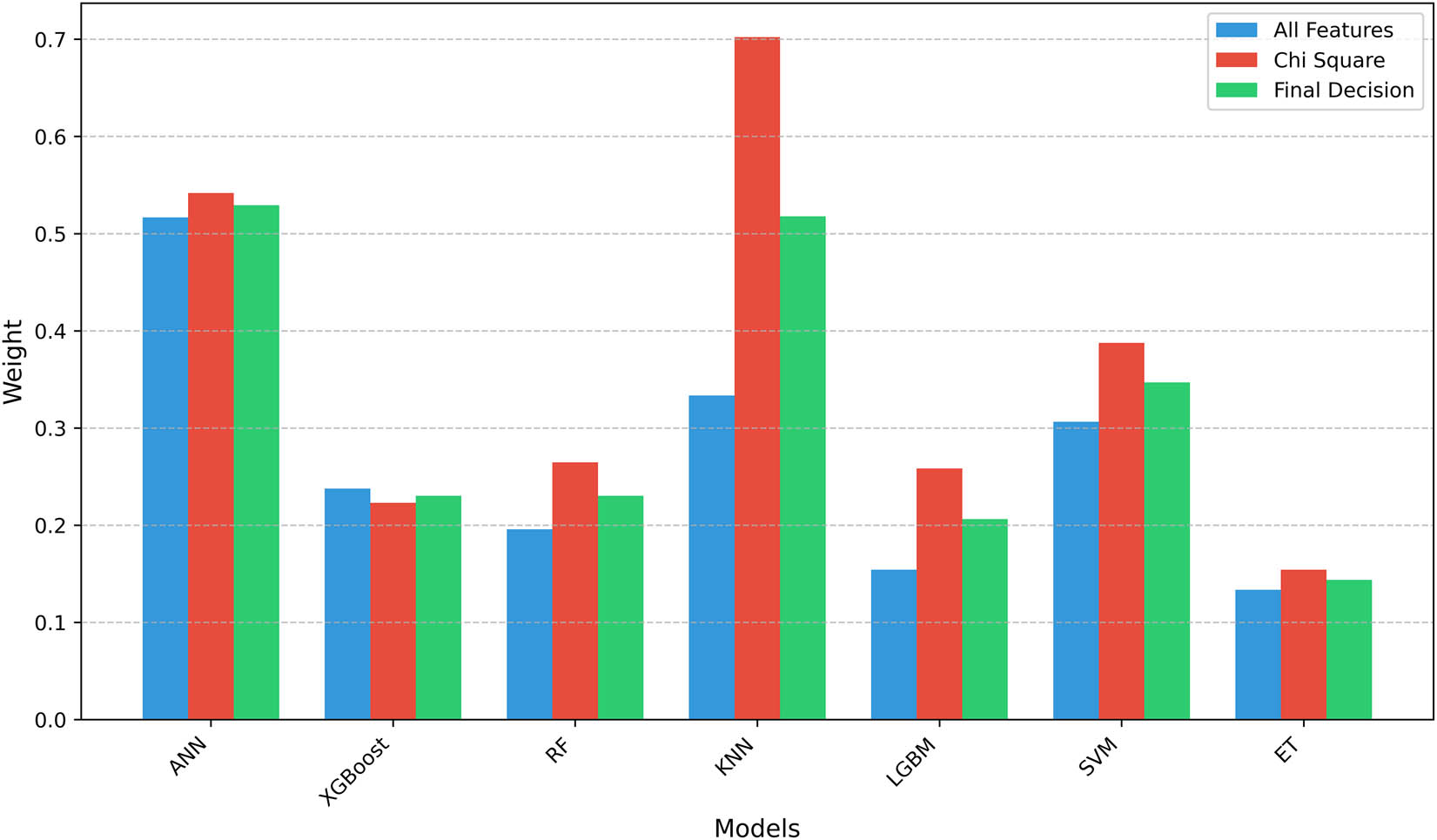
Comparison of model weights in different scenarios. The bars represent the relative performance scores (weights) of the algorithms, under three scenarios, which use all features, Chi-square, and the final decision (combined approach). Lower weights indicate better performance. Source: Created by the authors.
4.4 Explainable artificial intelligence (XAI)
XAI aims to make ML models more interpretable to humans and address complex models. One prominent technique within XAI is local interpretable model-agnostic explanations (LIME), which provides local explanations for individual predictions made by any ML model, regardless of its complexity. LIME works by generating perturbed versions of the input data and observing how the model predictions change. A simpler, interpretable model is subsequently trained on the perturbed data to locally approximate the complex model’s behaviour. This allows LIME to identify the most important features that influence a specific prediction, offering insights that are easier for humans to understand. According to FDOSM, the best algorithm is ET; then LIME will run through it and Chi-square to see the 20.
Table 14 shows the feature-level contribution of ICU patient survival prediction. The “Value” column indicates the specific instance of each feature for a given patient, while the “Contributions” column represents the influence of each feature on the model’s prediction. A positive contribution suggests that the feature is associated with the likelihood of survival, while a negative contribution indicates the opposite. The column “Belong to class” specifies whether the instance is classified as “Survives” or “non-survived,” providing a clear understanding of how the features impact the final classification outcome.
Feature contribution impact on model classification to ICU patient survival and non-survival prediction
| No | Feature | Value | Contribution | Class |
|---|---|---|---|---|
| 1 | ID | 0.00 | 0.0822 | Survival |
| 2 | Status.Discharge.first | 1.10 | 0.0738 | Survival |
| 3 | Diagnosis.seq | 0.64 | 0.0614 | Survival |
| 4 | PAtion | 1.72 | −0.0541 | Non-survival |
| 5 | ICD.Code.final | 1.95 | 0.0507 | Survival |
| 6 | Age | 4.14 | −0.0418 | Non-survival |
| 7 | final state | 0.85 | 0.0299 | Survival |
| 8 | Follow.Date | 1.34 | −0.0243 | Non-survival |
| 9 | AdmitDept | 0.76 | −0.0237 | Non-survival |
| 10 | InfectionSite | 0.79 | 0.0209 | Survival |
| 11 | ICU.discharge.time | 0.06 | −0.02040.0201 | Non-survival |
| 12 | state 1(first) | 1.26 | 0.0135 | Survival |
| 13 | DISCHARGE.DATE.TIME | 0.43 | 0.0125 | Survival |
| 14 | state3 | 0.38 | −0.0125 | Non-survival |
| 15 | stope reason | 0.59 | −0.0117 | Non-survival |
| 16 | ICD.Code.first | 1.51 | −0.0072 | Non-survival |
| 17 | Status.Discharge.final | 0.01 | −0.0061 | Non-survival |
| 18 | Sequence check | 0.77 | 0.0044 | Survival |
| 19 | SEX | 0.37 | 0.0041 | Survival |
| 20 | start reason | 1.14 | 0.0002 | Survival |
Figure 5 shows the predictive importance of the feature for patient survival outcomes using the ET algorithm. The left panel displays feature importance patterns derived close to survival, while the right panel shows the feature importance close to non-survival. Each horizontal bar represents a specific clinical feature, and the length of the bar indicates its relative importance in predicting whether a patient survived (blue bars) or did not survive (orange bars). The numerical values adjacent to each bar represent the normalized importance score for that feature within the respective model. The features are vertically ordered based on their overall importance in both survival outcomes.
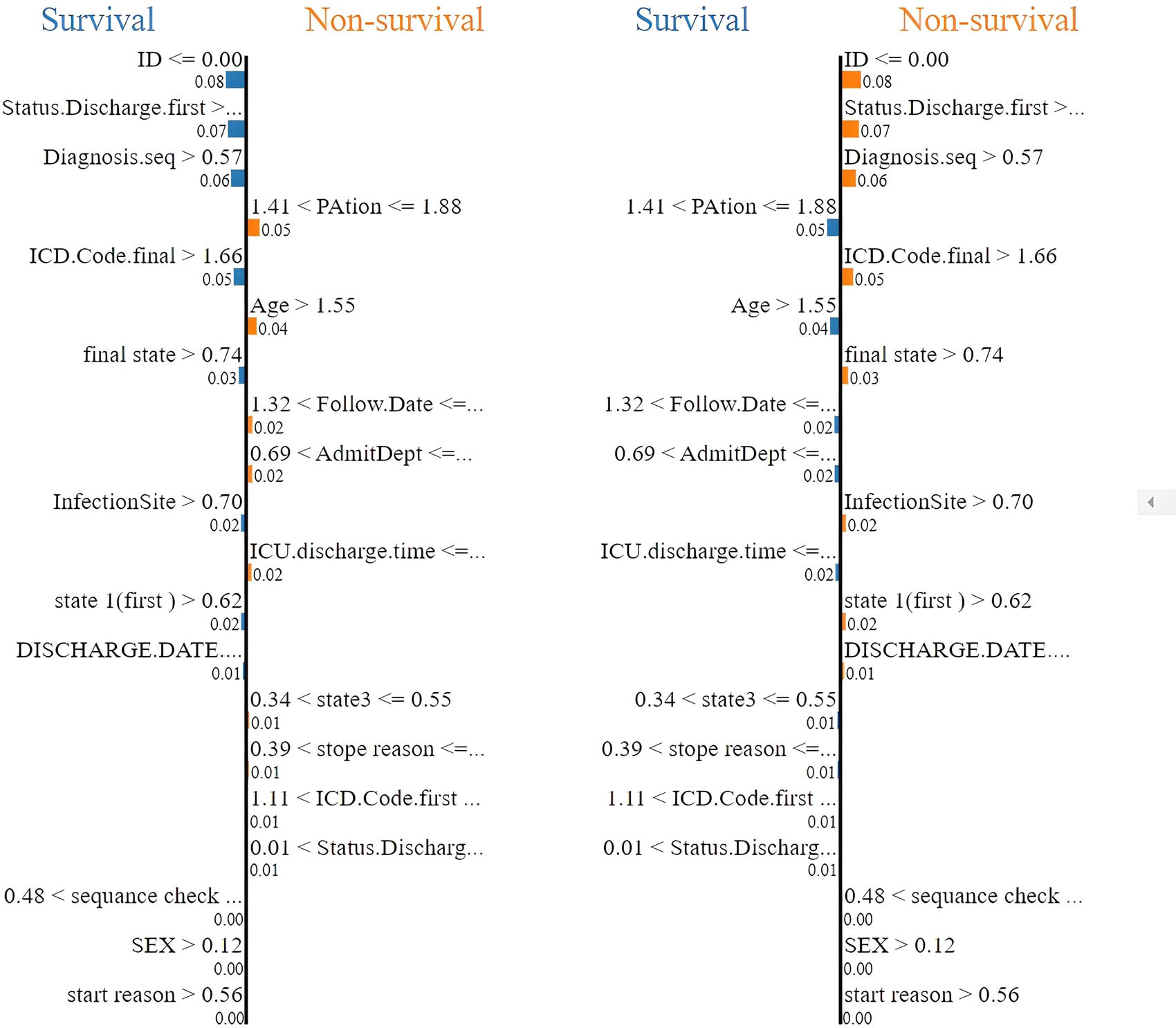
Comparison of the importance of survival prediction across the ET algorithm. Source: Created by the authors.
Figure 6 shows a LIME explanation for a single patient predicted to survive, illustrating the contributions of local features to this specific prediction. Red bars represent features that negatively influenced the prediction, pushing it towards “Non-survival,” including a specific range for “PAtion,” higher age, a high final-state value, and certain ranges for follow-up date and admission department. The predicted probability of survival for this patient is 0.67, while the probability of non-survival is 0.33. This instance-level explanation enhances the interpretability of the ET model decision-making by highlighting the most influential factors for this particular case, supporting trust-building and potential model debugging, although it represents exclusively a local view and may not reflect the model’s global behaviour.
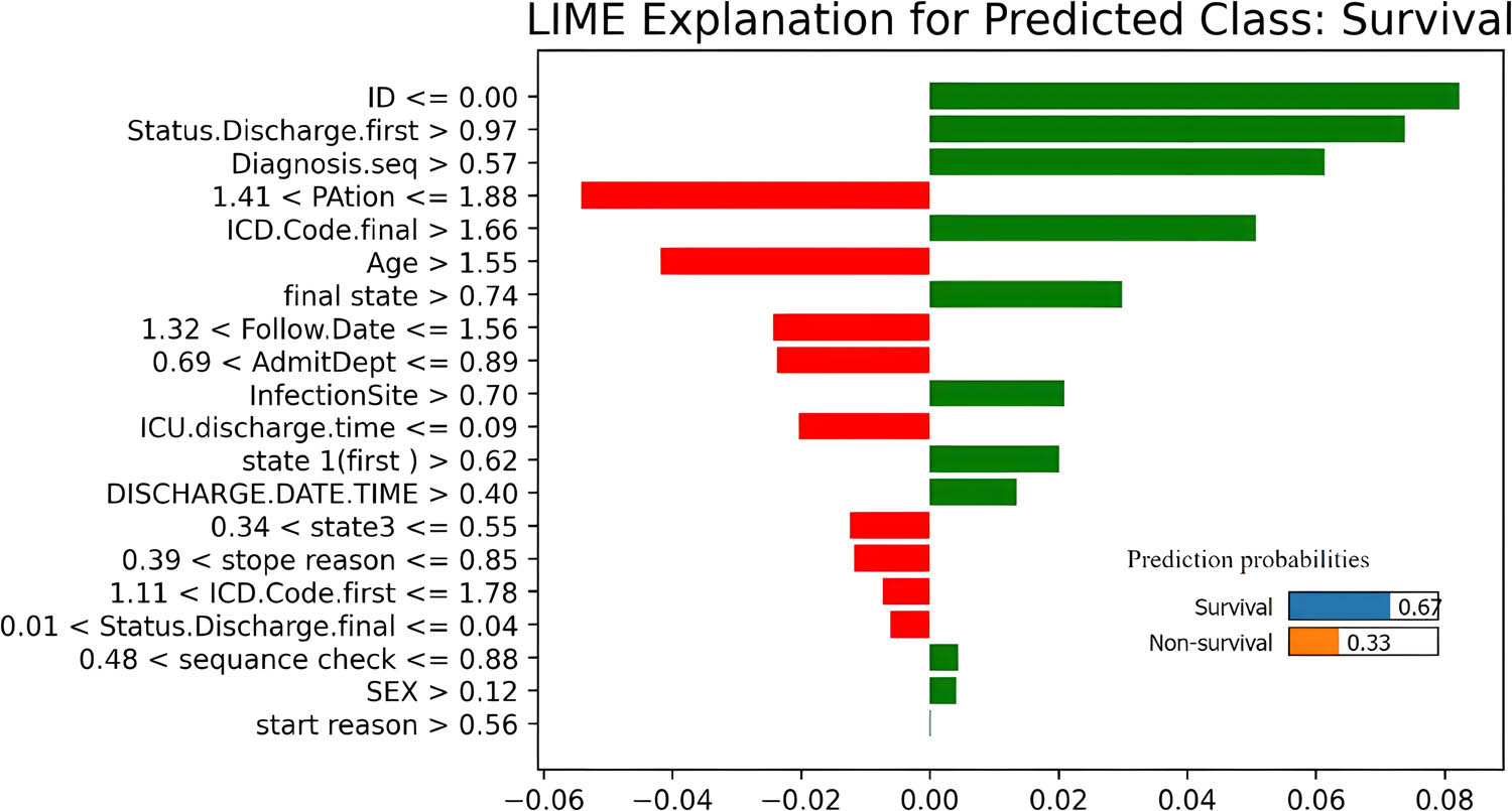
LIME explanation for a single instance predicted class with feature importance. Source: Created by the authors.
4.5 Comparison analysis
This analysis compares the performance of various ML algorithms under two different feature sets, which are all features (Table 8) and features selected using the Chi-square method (Table 10). The comparison focuses on key classification metrics, including precision, recall, F-score, Kappa statistic, AUC, MCC, and accuracy. The application of the Chi-square feature selection generally led to significant improvements across most evaluation metrics for all models. This suggests that eliminating irrelevant or redundant features can enhance classification performance, model generalizability, and interpretability. The following are key compressions:
In terms of precision and F-score, ET demonstrated the most notable improvement, with accuracy increasing from 83.471% to 88.167% and F-score from 86.239 to 87.886. XGBoost also showed significant gains, with its precision increasing from 82.094% to 87.935% and F-score from 85.327 to 87.963. Consistent patterns were observed in RF and LGBM, both of which showed solid improvements in F-score and accuracy, confirming their effectiveness in both high-dimensional and feature-reduced settings.
For the balance between precision and recall, SVM improved its precision from 79.325 to 90.206 after feature selection, but its recall dropped from 88.679 to 81.019, suggesting fewer false positives but more false negatives. KNN achieved peak precision of 89.032; however, its recall significantly decreased from 84.434 to 63.889, resulting in a lower F-score of 74.394. These differences indicate that although KNN became more precise, it may be less effective in identifying all relevant instances after feature reduction.
Analysing the reliability metrics, all models experienced an increase in Kappa and MCC scores after feature selection, reflecting improved model consistency and predictive power. ET again led with the highest Kappa (76.337) and MCC (76.436), underscoring its reliable and balanced classification performance in different classes.
Finally, the AUC metric, which measures the model’s ability to discriminate between classes, improved across all algorithms with feature selection. ET achieved the highest AUC of 88.173, closely followed by XGBoost and LGBM. These results confirm that ensemble-based models not only maintain their robustness after feature selection but actually perform better in ranking and classification tasks.
The application of chi-squared feature selection significantly enhances the performance of ML models. Ensemble methods, particularly ET, XGBoost, RF, and LGBM, demonstrate the greatest benefits in all evaluated metrics. Although KNN achieved high precision, its decreased recall suggests a potential risk of false negatives. Overall, ET stands out as the most effective and reliable model for the given classification task, achieving superior performance in almost all aspects. Figure 7 presents a comparative radar chart analysis of the performance of the ET algorithm using all features versus using the Chi-square. As shown, the ET algorithm improves across metrics, especially Kappa, AUC, MCC, and accuracy, when feature selection is applied.
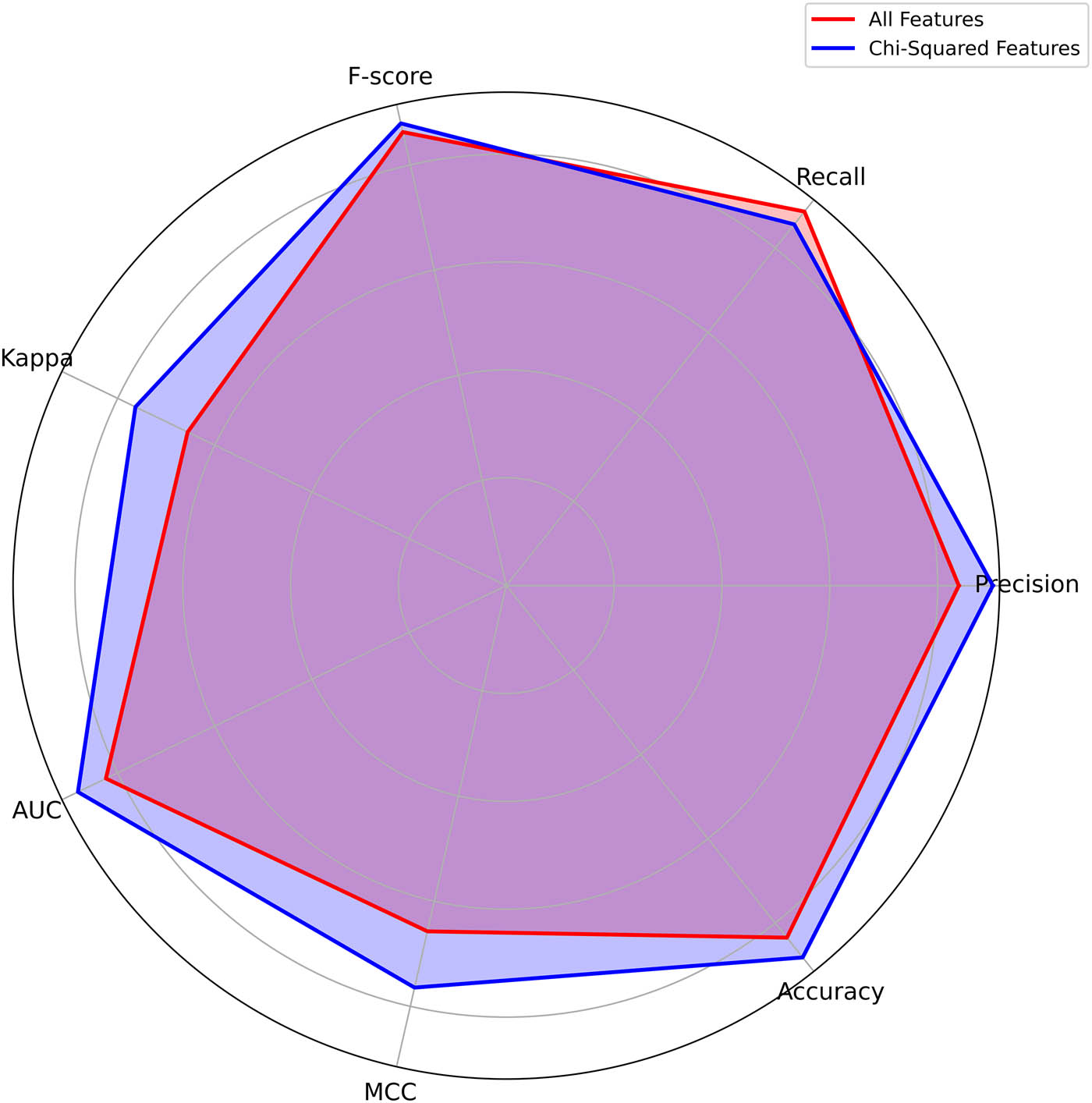
Radar chart comparison for the ET algorithm. Source: Created by the authors.
Recent advances in ICU mortality prediction demonstrated the potential of ML, yet trade-offs persist between evaluation metrics and interpretability. As demonstrated in Table 15, our proposed framework ML-FDOSM achieves superior precision and recall compared to state-of-the-art alternatives while maintaining high explainability through LIME integration. The comparison reveals three key trends: (i) hybrid methods [12] like ours, (ii) interpretability often correlates with implementation success more strongly than raw accuracy, and (iii) our Zigong ICU validation shows consistent improvements over prior work on similar datasets [1].
Performance comparison of our proposed framework ML-FDOSM against state-of-the-art ICU mortality prediction models
| Reference | Dataset | Precession | Recall | AUC | Accuracy | Interpretability |
|---|---|---|---|---|---|---|
| [8] | Surgical ICU | 85.4 | 82.4 | 91.3 | 84.2 | Medium |
| [1] | Zigong ICU | 86.957 | 80.645 | — | 86.411 | Medium (visualization) |
| [12] | MIMIC-III | 87.2 | 83.7 | 92.6 | 86.3 | Medium |
| [9] | Mixed ICU | 83.1 | 80.1 | 89 | 82.4 | Low (black box) |
| Our work | Zigong ICU | 90.244 | 85.648 | 88.173 | 88.167 | High (LIME) |
While this study provides valuable insights, several limitations require consideration in future investigations. First, the dataset used for model training and evaluation was obtained from a single ICU setting, Zigong Fourth People’s Hospital, which may restrict the generalizability of the findings to other hospitals, including those in different regions or specialized units such as pediatric ICUs. Second, although imputation techniques were used to handle missing values, estimating missing clinical data inherently introduces uncertainty. Third, the current approach relies on batch processing of ICU data, and the performance in real-time environments has not yet been fully explored. To address these limitations, future work should focus on validating the model using multicentre datasets to enhance robustness and generalizability. Additionally, the incorporation of advanced techniques such as self-supervised or reinforcement learning may offer more effective strategies for managing missing data. Further evaluation is also needed to assess computational efficiency and adapt the model for real-time clinical decision support.
5 Conclusions
This study successfully establishes the effectiveness of integrating ML with FDOSM to improve early mortality prediction for patients in the ICU. Using a comprehensive dataset from Zigong Fourth People’s Hospital, feature selection using Chi-square and seven ML models, we developed a robust hybrid model that improves accuracy, interpretability, and clinical utility of mortality forecasts. The results showed notable improvements in performance in several metrics, with ET emerging as the most effective algorithm, achieving the highest accuracy (88.167%), precision (90.244%), and AUC (88.173%) after feature selection. Ensemble methods, particularly ET, XGBoost, RF, and LGBM, demonstrated significant gains, particularly in F-score and AUC, reinforcing their strength in handling high-dimensional clinical data. However, the study’s limitations include the reliance on a single ICU dataset, potential uncertainties introduced by imputation techniques for missing data, and the lack of real-time model evaluation. These factors point to avenues for future work, such as validating the model with multicentre datasets, exploring advanced data handling techniques, and adapting the model for real-time clinical applications.
-
Funding information: No funding was received for conducting this study.
-
Author contributions: Kareem Hameed Khalaf conceptualized the study and performed the experiments. Abdolhamid Moallemi Khiavi was responsible for data preprocessing and model evaluation and also served as a corresponding author, providing supervision and handling manuscript correspondence. Dhafar Hamed Abd contributed to the final manuscript review and also served as a corresponding author, managing revisions and communication with the journal. All authors approved the final version.
-
Conflict of interest: The authors state no conflict of interest.
-
Data availability statement: The data supporting the findings of this study are openly available in PhysioNet repository at https://doi.org/10.13026/gz5h-e561.
References
[1] Khalaf KH, Khiavi AM, Abd DH. Adversarial ensemble learning for mortality prediction in intensive care units. 2024 17th International Conference on Development in eSystem Engineering (DeSE). IEEE; 2024. p. 405–10. 10.1109/DeSE63988.2024.10912041.Search in Google Scholar
[2] Czapla M, Juárez-Vela R, Gea-Caballero V, Zieliński S, Zielińska M. The association between nutritional status and in-hospital mortality of COVID-19 in critically-ill patients in the ICU. Nutrients. 2021;13(10):3302. 10.3390/nu13103302.Search in Google Scholar PubMed PubMed Central
[3] Hourmant Y, Mailloux A, Valade S, Lemiale V, Azoulay E, Darmon M. Impact of early ICU admission on outcome of critically ill and critically ill cancer patients: A systematic review and meta-analysis. J Crit Care. 2021;61:82–8. 10.1016/j.jcrc.2020.10.008.Search in Google Scholar PubMed
[4] Churpek MM, Gupta S, Spicer AB, Parker WF, Fahrenbach J, Brenner SK, et al. Hospital-level variation in death for critically ill patients with COVID-19. Am J Respir Crit Care Med. 2021;204(4):403–11. 10.1164/rccm.202012-4547OC.Search in Google Scholar PubMed PubMed Central
[5] Grasselli G, Scaravilli V, Mangioni D, Scudeller L, Alagna L, Bartoletti M, et al. Hospital-acquired infections in critically ill patients with COVID-19. Chest. 2021;160(2):454–65. 10.1016/j.chest.2021.04.002.Search in Google Scholar PubMed PubMed Central
[6] Kiekkas P, Tzenalis A, Gklava V, Stefanopoulos N, Voyagis G, Aretha D. Delayed admission to the intensive care unit and mortality of critically ill adults: Systematic review and meta‐analysis. BioMed Res Int. 2022;2022(1):4083494. 10.1155/2022/4083494.Search in Google Scholar PubMed PubMed Central
[7] Silveira EC, Pretti SM, Santos BA, Corrêa CFS, Silva LM, de Melo FF. Prediction of hospital mortality in intensive care unit patients from clinical and laboratory data: A machine learning approach. World J Crit Care Med. 2022;11(5):317. 10.5492/wjccm.v11.i5.317.Search in Google Scholar PubMed PubMed Central
[8] Yun K, Oh J, Hong TH, Kim EY. Prediction of mortality in surgical intensive care unit patients using machine learning algorithms. Front Med. 2021;8:621861. 10.3389/fmed.2021.621861.Search in Google Scholar PubMed PubMed Central
[9] Chiu C-C, Wu C-M, Chien T-N, Kao L-J, Qiu JT. Predicting the mortality of ICU patients by topic model with machine-learning techniques. Healthcare. 2022;10(6):1087. 10.3390/healthcare10061087.Search in Google Scholar PubMed PubMed Central
[10] Quinto B. Introduction to machine learning. Next-generation machine learning with spark: Covers XGBoost, LightGBM, Spark NLP, distributed deep learning with keras, and more. Springer; 2020. p. 1–27. 10.1007/978-1-4842-5669-5.Search in Google Scholar
[11] Shamout F, Zhu T, Clifton DA. Machine learning for clinical outcome prediction. IEEE Rev Biomed Eng. 2020;14:116–26. 10.1109/RBME.2020.3007816.Search in Google Scholar PubMed
[12] Mansouri A, Noei M, Saniee Abadeh M. A hybrid machine learning approach for early mortality prediction of ICU patients. Prog Artif Intell. 2022;11(4):333–47. 10.1007/s13748-022-00288-0.Search in Google Scholar
[13] Caicedo-Torres W, Gutierrez J. ISeeU: Visually interpretable deep learning for mortality prediction inside the ICU. J Biomed Inform. 2019;98:103269. 10.1016/j.jbi.2019.103269.Search in Google Scholar PubMed
[14] Abd DH, Al-Mejibli IS. Monitoring system for sickle cell disease patients by using supervised machine learning. 2017 Second Al-Sadiq International Conference on Multidisciplinary in IT and Communication Science and Applications (AIC-MITCSA). IEEE; 2017. p. 119–4. 10.1109/AIC-MITCSA.2017.8723006.Search in Google Scholar
[15] Zilker S, Weinzierl S, Kraus M, Zschech P, Matzner M. A machine learning framework for interpretable predictions in patient pathways: The case of predicting ICU admission for patients with symptoms of sepsis. Health Care Manag Sci. 2024;27(2):136–67. 10.1007/s10729-024-09673-8.Search in Google Scholar PubMed PubMed Central
[16] Mukhlif DM, Abd DH, Ejbali R, Alimi AM, Mahdi MF. Enhancing comorbidity diagnosis with adversarial ensemble learning. 2024 17th International Conference on Development in eSystem Engineering (DeSE). IEEE; 2024. p. 381–6. 10.1109/DeSE63988.2024.10912032.Search in Google Scholar
[17] Ghazi RF, Abd DH. Gene disease classification from biomedical text via ensemble machine learning. 2023 16th International Conference on Developments in eSystems Engineering (DeSE). IEEE; 2023. p. 593–8. 10.1109/DeSE60595.2023.10469108.Search in Google Scholar
[18] Nsaif AA, Abd DH. Sentiment analysis of political post classification based on XGBoost. Proceedings of International Conference on Computing and Communication Networks: ICCCN 2021. Singapore: Springer Nature Singapore; 2022. p. 177–88. 10.1007/978-981-19-0604-6_16.Search in Google Scholar
[19] Jassim MA, Abd DH, Omri MN. Machine learning-based new approach to films review. Soc Netw Anal Min. 2023;13(1):40. 10.1007/s13278-023-01042-7.Search in Google Scholar
[20] Mukhlif DM, Abd DH, Ejbali R, Alimi AM, Mahdi MF, Hussain AJ. Comorbidity diagnosis using machine learning: Fuzzy decision-making approach. J Intell Syst. 2025;34(1):20240418. 10.1515/jisys-2024-0418.Search in Google Scholar
[21] Siöland T, Rawshani A, Nellgård B, Malmgren J, Oras J, Dalla K, et al. ICURE: Intensive care unit (ICU) risk evaluation for 30‐day mortality. Developing and evaluating a multivariable machine learning prediction model for patients admitted to the general ICU in Sweden. Acta Anaesthesiol Scand. 2024;68(10):1379–89. 10.1111/aas.14501.Search in Google Scholar PubMed
[22] Ko R-E, Cho J, Shin M-K, Oh SW, Seong Y, Jeon J, et al. Machine learning-based mortality prediction model for critically Ill Cancer patients admitted to the Intensive Care Unit (CanICU). Cancers. 2023;15(3):569. 10.3390/cancers15030569.Search in Google Scholar PubMed PubMed Central
[23] Razo M, Pishgar M, Galanter W, Darabi H. Deep-learning model for mortality prediction of ICU patients with paralytic ileus. Bioengineering. 2024;11(12):1214. 10.3390/bioengineering11121214.Search in Google Scholar PubMed PubMed Central
[24] Tu K-C, Tau ENT, Chen N-C, Chang M-C, Yu T-C, Wang C-C, et al. Machine learning algorithm predicts mortality risk in intensive care unit for patients with traumatic brain injury. Diagnostics. 2023;13(18):3016. 10.3390/diagnostics13183016.Search in Google Scholar PubMed PubMed Central
[25] Tasnim N, Al Mamun S, Shahidul Islam M, Kaiser MS, Mahmud M. Explainable mortality prediction model for congestive heart failure with nature-based feature selection method. Appl Sci. 2023;13(10):6138. 10.3390/app13106138.Search in Google Scholar
[26] Yu Z, Fang L, Ding Y. Explainable machine learning model for prediction of 28-day all-cause mortality in immunocompromised patients in the intensive care unit: a retrospective cohort study based on MIMIC-IV database. Eur J Med Res. 2025;30(1):358. 10.1186/s40001-025-02622-3.Search in Google Scholar PubMed PubMed Central
[27] Prithula J, Chowdhury ME, Khan MS, Al-Ansari K, Zughaier SM, Islam KR, et al. Improved pediatric ICU mortality prediction for respiratory diseases: Machine learning and data subdivision insights. Respir Res. 2024;25(1):216. 10.1186/s12931-024-02753-x.Search in Google Scholar PubMed PubMed Central
[28] Xu P, Chen L, Zhu Y, Yu S, Chen R, Huang W, et al. Critical care database comprising patients with infection. Front Public Health. 2022;10:852410. 10.3389/fpubh.2022.852410.Search in Google Scholar PubMed PubMed Central
[29] Ferreira FL, Bota DP, Bross A, Mélot C, Vincent J-L. Serial evaluation of the SOFA score to predict outcome in critically ill patients. JAMA. 2001;286(14):1754–8. 10.1001/jama.286.14.1754.Search in Google Scholar PubMed
[30] Raouf ZT, Abd DH. Feature selection for binary dataset using dragonfly algorithm. 2023 16th International Conference on Developments in eSystems Engineering (DeSE). IEEE; 2023. p. 480–5. 10.1109/DeSE60595.2023.10469222.Search in Google Scholar
[31] Mukhlif DM, Abd DH, Ejbali R, Alimi AM. Comorbidity diseases diagnosis using machine learning methods and chi-square feature selection technique. 2023 16th International Conference on Developments in eSystems Engineering (DeSE). IEEE; 2023. p. 144–9. 10.1109/DeSE60595.2023.10469092.Search in Google Scholar
[32] Ahmed AA, Hasan MK, Jaber MM, Al-Ghuribi SM, Abd DH, Khan W, et al. Arabic text detection using rough set theory: Designing a novel approach. IEEE Access. 2023;11:68428–38. 10.1109/ACCESS.2023.3278272.Search in Google Scholar
[33] Abd DH, Khan W, Khan B, Alharbe N, Al-Jumeily D, Hussain A. Categorization of Arabic posts using Artificial Neural Network and hash features. J King Saud Univ-Sci. 2023;35(6):102733. 10.1016/j.jksus.2023.102733.Search in Google Scholar
[34] Salih MM, Zaidan B, Zaidan A. Fuzzy decision by opinion score method. Appl Soft Comput. 2020;96:106595. 10.1016/j.asoc.2020.106595.Search in Google Scholar
[35] Albahri OS, Zaidan AA, Salih MM, Zaidan BB, Khatari MA, Ahmed MA, et al. Multidimensional benchmarking of the active queue management methods of network congestion control based on extension of fuzzy decision by opinion score method. Int J Intell Syst. 2021;36(2):796–831. 10.1002/int.22322.Search in Google Scholar
[36] Al-Qaysi Z, Albahri A, Ahmed M, SM, Mohammed. Development of hybrid feature learner model integrating FDOSM for golden subject identification in motor imagery. Phys Eng Sci Med. 2023;46(4):1519–34. 10.1007/s13246-023-01316-6.Search in Google Scholar PubMed
© 2025 the author(s), published by De Gruyter
This work is licensed under the Creative Commons Attribution 4.0 International License.
Articles in the same Issue
- Research Articles
- Synergistic effect of artificial intelligence and new real-time disassembly sensors: Overcoming limitations and expanding application scope
- Greenhouse environmental monitoring and control system based on improved fuzzy PID and neural network algorithms
- Explainable deep learning approach for recognizing “Egyptian Cobra” bite in real-time
- Optimization of cyber security through the implementation of AI technologies
- Deep multi-view feature fusion with data augmentation for improved diabetic retinopathy classification
- A new metaheuristic algorithm for solving multi-objective single-machine scheduling problems
- Estimating glycemic index in a specific dataset: The case of Moroccan cuisine
- Hybrid modeling of structure extension and instance weighting for naive Bayes
- Application of adaptive artificial bee colony algorithm in environmental and economic dispatching management
- Stock price prediction based on dual important indicators using ARIMAX: A case study in Vietnam
- Emotion recognition and interaction of smart education environment screen based on deep learning networks
- Supply chain performance evaluation model for integrated circuit industry based on fuzzy analytic hierarchy process and fuzzy neural network
- Application and optimization of machine learning algorithms for optical character recognition in complex scenarios
- Comorbidity diagnosis using machine learning: Fuzzy decision-making approach
- A fast and fully automated system for segmenting retinal blood vessels in fundus images
- Application of computer wireless network database technology in information management
- A new model for maintenance prediction using altruistic dragonfly algorithm and support vector machine
- A stacking ensemble classification model for determining the state of nitrogen-filled car tires
- Research on image random matrix modeling and stylized rendering algorithm for painting color learning
- Predictive models for overall health of hydroelectric equipment based on multi-measurement point output
- Architectural design visual information mining system based on image processing technology
- Measurement and deformation monitoring system for underground engineering robots based on Internet of Things architecture
- Face recognition method based on convolutional neural network and distributed computing
- OPGW fault localization method based on transformer and federated learning
- Class-consistent technology-based outlier detection for incomplete real-valued data based on rough set theory and granular computing
- Detection of single and dual pulmonary diseases using an optimized vision transformer
- CNN-EWC: A continuous deep learning approach for lung cancer classification
- Cloud computing virtualization technology based on bandwidth resource-aware migration algorithm
- Hyperparameters optimization of evolving spiking neural network using artificial bee colony for unsupervised anomaly detection
- Classification of histopathological images for oral cancer in early stages using a deep learning approach
- A refined methodological approach: Long-term stock market forecasting with XGBoost
- Enhancing highway security and wildlife safety: Mitigating wildlife–vehicle collisions with deep learning and drone technology
- An adaptive genetic algorithm with double populations for solving traveling salesman problems
- EEG channels selection for stroke patients rehabilitation using equilibrium optimizer
- Influence of intelligent manufacturing on innovation efficiency based on machine learning: A mechanism analysis of government subsidies and intellectual capital
- An intelligent enterprise system with processing and verification of business documents using big data and AI
- Hybrid deep learning for bankruptcy prediction: An optimized LSTM model with harmony search algorithm
- Construction of classroom teaching evaluation model based on machine learning facilitated facial expression recognition
- Artificial intelligence for enhanced quality assurance through advanced strategies and implementation in the software industry
- An anomaly analysis method for measurement data based on similarity metric and improved deep reinforcement learning under the power Internet of Things architecture
- Optimizing papaya disease classification: A hybrid approach using deep features and PCA-enhanced machine learning
- Handwritten digit recognition: Comparative analysis of ML, CNN, vision transformer, and hybrid models on the MNIST dataset
- Multimodal data analysis for post-decortication therapy optimization using IoMT and reinforcement learning
- Predicting early mortality for patients in intensive care units using machine learning and FDOSM
- Uncertainty measurement for a three heterogeneous information system based on k-nearest neighborhood: Application to unsupervised attribute reduction
- Review Articles
- A comprehensive review of deep learning and machine learning techniques for early-stage skin cancer detection: Challenges and research gaps
- An experimental study of U-net variants on liver segmentation from CT scans
- Strategies for protection against adversarial attacks in AI models: An in-depth review
- Resource allocation strategies and task scheduling algorithms for cloud computing: A systematic literature review
- Latency optimization approaches for healthcare Internet of Things and fog computing: A comprehensive review
- Explainable clustering: Methods, challenges, and future opportunities