Stability Problems and Analytical Integration for the Clebsch’s System
-
Camelia Pop


Abstract
The nonlinear stability and the existence of periodic orbits of the equilibrium states of the Clebsch’s system are discussed.. Numerical integration using the Lie-Trotter integrator and the analytic approximate solutions using Multistage Optimal Homotopy Asymptotic Method are presented, too.
1 Introduction
The Clebsch’s system was proposed in 1870 (see [1] for details) and it represents a specific famous case of the Kirchoff equations which describes the motion of a rigid body in an ideal fluid. The Clebsch’s case was obtained from the equations:
by taking the quadratic Hamiltonian
where
The physical meaning of p is the total angular momentum, whereas x represents the total linear momentum of the system.
If we consider now the Hamiltonian
the equations (1) become:
where a1, a2, a3 are different and nonzero constants. It is well-known that its first integrals are:
and
During the time since its publication, a lot of problems about the Clebsch’s system have been studied like its almost Lie-Poisson structure ([2]), the Lax formulation ([3]) or its Hirota-Kimura type discretization ([4]).
The paper’s structure is as follows: first, the nonlinear stability of the equilibrium states of Clebsch’s dynamics is discussed. About this problem, only partial results were found in [2] due to the fact that the existence of a Hamilton-Poisson structure is still an open problem, and for the almost Hamilton-Poisson structure proposed only one Casimir function was found instead of two. We use here the Arnold’s method in order to obtain some new results, which does not require a Hamilton-Poisson structure. The existence of the periodic orbits around the nonlinear stable states is the subject of the second part. The last part is committed to the numerical and analytical integration. Two methods are proposed: the Lie-Trotter integrator for numerical integration and the Multistage Optimal Homotopy Asymptotic Method to find the analytic approximate solutions. Numerical simulations obtained via Mathematica 10 are presented, too.
2 Stability problems
The equilibrium states of the dynamics (3) are
Proposition 1
If a1 < a2 and a1 < a3 then the equilibrium states
Proof
We shall make the proof using Arnold’s method ([5]).
Let Fα,β,γ ∈ C∞ (R6, R) given by
Following Arnold’s method, we have successively:
∇Fα,β,γ(
Considering the space
then
for any v ∈ X, i.e.
is positive definite if a1 < a2 and a1 < a3. □
□
Using the same arguments we obtain the following results:
Proposition 2
The equilibrium states
Proposition 3
The equilibrium states
Proposition 4
The equilibrium states
Proof
For this case we consider the function Gα,β ∈ C∞ (R6, R),
Following Arnold’s method, we have successively:
∇Gα,β(
Let us consider the space
then
for any v ∈ Y, i.e.
is positive definite.□
□
3 Periodic orbits
Proposition 5
If a1 < a2 and a1 < a3 then, near to
Proof
We use the Moser-Weinstein theorem with zero eigenvalue, see [6] for details:
The restriction of our dynamics (3) to the coadjoint orbit:
gives rise to a classical Hamiltonian system.
The matrix of the linear part of the reduced dynamics is:
and has purely imaginary roots. More exactly:
span (∇H2(
The smooth function F1−a1,−1,0 ∈ C∞ (R6, R) given by
has the following properties:
It is a constant of motion of the dynamics (3).
∇F1−a1,−1,0(
If a1 < a2 and a1 < a3 then
where
Then our assertion follows. □
Using similar arguments, the following results hold:
Proposition 6
If a2 < a1 and a2 < a3 then near to
Proposition 7
If a3 < a1 and a3 < a2 then near to
Remark 1
The existence of periodic orbits around the equilibrium states
4 Numerical integration
We shall discuss now the numerical integration of the equations (3) via the Lie-Trotter formula ([7]).
Figures 1 and 2 present numerical simulations obtained with MATHEMATICA 10.
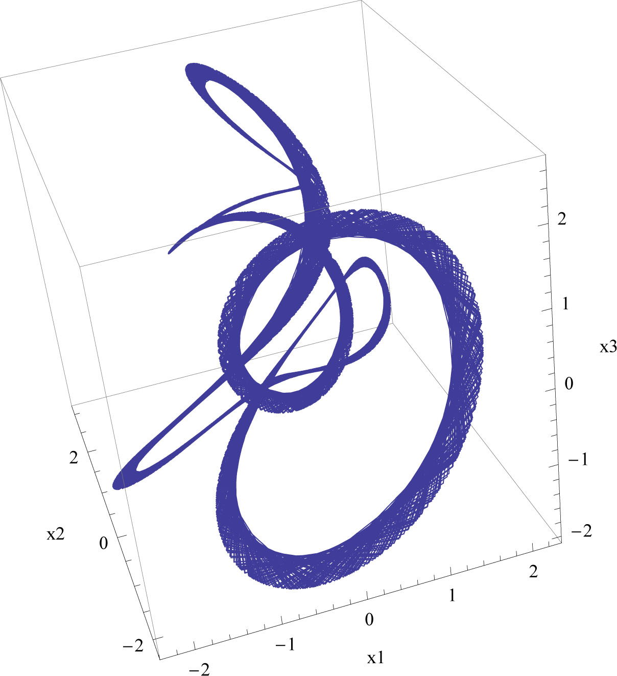
The Lie-Trotter integrator of the system (3), projection on (Ox1x2x3) plane (a1 = 10, a2 = 2, a3 = 3, x1(0) = x2(0) = x3(0) = p1(0) = p2(0) = p3(0) = 1).
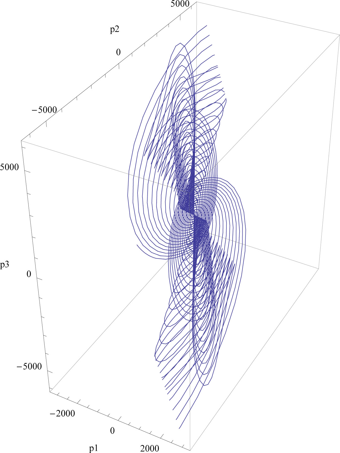
The Lie-Trotter integrator of the system (3), projection on (Op1p2p3) plane (a1 = 10, a2 = 2, a3 = 3, x1(0) = x2(0) = x3(0) = p1(0) = p2(0) = p3(0) = 1).
Following [2] or [7], the Lie-Trotter integrator can be written as:
where
Some of its properties are sketched in the following proposition:
Proposition 8
The numerical integrator (4) preserves the Hamiltonians H1, H2, H3 and H4 if
and
5 Analytic approximate solutions of the Clebsch System (3) using Multistage Optimal Homotopy Asymptotic Method
In order to find the analytical approximate solutions of the nonlinear differential system (3) with the boundary conditions
we will use the Multistage Optimal Homotopy Asymptotic Method (MOHAM) [8], as follows:
we divide the theoretical interval [t0, T] into some subintervals as [t0, t1), …, [tj−1, tj), …, where tj = T;
The initial approximation in each interval [tj−1, tj), j ∈ ℕ* is provided by the solution from the previous interval, so the analytical approximate solutions can be obtained for equations of the general form
subject to the initial conditions (5), where 𝓛 is a linear operator (which is not unique) and 𝓝 is a nonlinear one.
Now, choosing the linear operators 𝓛 as:
and the nonlinear operators 𝓝[xi(t)] and 𝓝[pi(t)], i = 1, 3 as
b1, b2, b3 ∈ R, and following [9, 10] we are able to construct the homotopy given by:
where p ∈ [0, 1] is the embedding parameter, and H(t, Ci) ≠ 0 is an auxiliary convergence-control function, depending of the variable t and the parameters C1, C2, …, Cs.
The following properties hold:
and
For the functions F of the form
the following relation is obtained:
Considering the homotopy 𝓗 given by:
and using the linear operator given by Eq. (7), the solutions of the equation
for the initial approximations xi0 and pi0, i = 1, 3 respectively, are
where
The secular terms must be equal to zero, i.e.:
and
respectively.
Also, to compute F1(t, Ci) we solve the equation
by taking into consideration that the nonlinear operator N presents the general form:
where m is a positive integer and hi(η) and gi(η) are known functions depending both on F0(η) and 𝓝.
Substituting Eqs. (16) into Eqs. (8), we obtain
Now, we observe that the nonlinear operators 𝓝[xi0(t)] and 𝓝[pi0(t)], i = 1, 3 respectively, are linear combinations of the functions
Although the equation (17) is a nonhomogeneous linear one, in most cases its solution cannot be found. In order to compute the function F1(t, Ci) we will use the third modified version of OHAM (see [9] for details), consisting of the following steps:
We choose the auxiliary convergence-control functions Hi such that Hi ⋅ 𝓝[F0(t)] and 𝓝[F0(t)] have the same form. So, the first approximation of xi1 or pi1, i = 1, 3, denoted F1, becomes:
where
Finally, the convergence-control parameters ω0, ω1 - ω6, B1-B12, C1-C12, which determine the first-order approximate solution (21), can be optimally computed by means of various methods, such as: the least square method, the Galerkin method, the collocation method, the Kantorowich method or the weighted residual method.
6 Numerical Examples and Discussions
In this section, the accuracy and validity of the MOHAM technique is proved using a comparison of our approximate solutions with numerical results obtained via the fourth-order Runge-Kutta method in the following case: we consider the initial value problem given by (3) with initial conditions Ai = 1, i = 1, 6, a1 = 10, a2 = 2 and a3 = 3.
The convergence-control parameters b1, b2, b3, ω0, ω1 - ω6,
For x̄1 : the convergence-control parameters on the interval [0, 2] are:
and the convergence-control parameters on the interval [2, 5] are given by:
for x̄2 : the convergence-control parameters on the interval [0, 2] are:
and the convergence-control parameters on the interval [2, 5] are given by:
for x̄3 : the convergence-control parameters on the interval [0, 2] are:
and the convergence-control parameters on interval [2, 5] are:
for p̄1 : the convergence-control parameters on the interval [0, 2] are:
and the convergence-control parameters on the interval [2, 5] are:
for p̄2 : the convergence-control parameters on the interval [0, 2] are:
and the convergence-control parameters on the interval [2, 5] are:
for p̄3 : the convergence-control parameters on the interval [0, 2] are:
and the convergence-control parameters on the interval [2, 5] are:
Finally, Tables 1 - 4 emphasizes the accuracy of the MOHAM technique by comparing the approximate analytic solutions x̄1 and p̄1 respectively presented above with the corresponding numerical integration values (via the 4th-order Runge-Kutta method), and the Lie-Trotter integrator. Finally, the results obtained using MOHAM are much closer to the original solution in comparison to the results obtained using Lie-Trotter integrator. These comparisons show the effectiveness, reliability, applicability, efficiency and accuracy of the MOHAM against to the Lie-Trotter integrator.
The comparison between the approximate solutions x̄1 given by Eq. (22) and the corresponding numerical solutions for a1 = 10, a2 = 2 and a3 = 3 (relative errors: ϵx1 = |x1numerical − x̄1MOHAM|)
| t | x1numerical | x1 | x̄1MOHAM | ϵx1 |
|---|---|---|---|---|
| Lie-Trotter (5 iterations) | given by Eq. (22) on [0, 2] | MOHAM | ||
| 0 | 1 | 1 | 1 | 0 |
| 1/5 | 0.7337023135 | 0.3397255522 | 0.7337010385 | 1.27 ⋅ 10−6 |
| 2/5 | 0.1051371952 | -0.1175841263 | 0.1051376412 | 4.46 ⋅ 10−7 |
| 3/5 | -0.5390294341 | 0.4802310232 | -0.5390162606 | 1.31 ⋅ 10−5 |
| 4/5 | -0.7408940837 | 1.0112524913 | -0.7408685929 | 2.54 ⋅ 10−5 |
| 1 | -0.1865095491 | 0.6934561430 | -0.1864820575 | 2.74 ⋅ 10−5 |
| 6/5 | 0.6179798375 | -0.0704392741 | 0.6180122798 | 3.24 ⋅ 10−5 |
| 7/5 | 0.7542356906 | -0.7051643433 | 0.7542576320 | 2.19 ⋅ 10−5 |
| 8/5 | 0.1623850803 | -1.0253085094 | 0.1623984362 | 1.33 ⋅ 10−5 |
| 9/5 | -0.5946553094 | -0.9561760501 | -0.5946418649 | 1.34 ⋅ 10−5 |
| 2 | -0.7270211941 | -0.3650442893 | -0.7269848249 | 3.63 ⋅ 10−5 |
The comparison between the approximate solutions x̄1 given by Eq. (23) and the corresponding numerical solutions for a1 = 10, a2 = 2 and a3 = 3 (relative errors: ϵx1 = |x1numerical − x̄1MOHAM|)
| t | x1numerical | x1 | x̄1MOHAM | ϵx1 |
|---|---|---|---|---|
| Lie-Trotter (5 iterations) | given by Eq. (23) on [2, 5] | MOHAM | ||
| 2 | -0.7270211941 | -0.3650442893 | -0.7269848249 | 3.63 ⋅ 10−5 |
| 23/10 | 0.4372022188 | 0.9364250346 | 0.4372037377 | 1.51 ⋅ 10−6 |
| 13/5 | 0.6086980787 | 0.3097132458 | 0.6088280862 | 1.30 ⋅ 10−4 |
| 29/10 | -0.5357138405 | -0.8052294850 | -0.5357087054 | 5.13 ⋅ 10−6 |
| 16/5 | -0.5145382567 | 1.5523267940 | -0.5143525655 | 1.85 ⋅ 10−4 |
| 7/2 | 0.6856064084 | 1.4821107514 | 0.6858827501 | 2.76 ⋅ 10−4 |
| 19/5 | 0.3181857442 | -1.2076590809 | 0.3183075232 | 1.21 ⋅ 10−4 |
| 41/10 | -0.7368863901 | -0.3502332442 | -0.7367419022 | 1.44 ⋅ 10−4 |
| 22/5 | -0.1421700459 | 0.5798310108 | -0.1420135462 | 1.56 ⋅ 10−4 |
| 47/10 | 0.7752628531 | 0.9869474224 | 0.7751771539 | 8.5 ⋅ 10−5 |
| 5 | -0.0560490264 | 0.7281825005 | -0.0561680013 | 1.18 ⋅ 10−4 |
The comparison between the approximate solutions p̄1 given by Eq. (28) and the corresponding numerical solutions for a1 = 10, a2 = 2 and a3 = 3 (relative errors: ϵp1 = |p1numerical − p̄1MOHAM|)
| t | p1numerical | p1 | p̄1MOHAM | ϵp1 |
|---|---|---|---|---|
| Lie-Trotter (5 iterations) | given by Eq. (28) on [0, 2] | MOHAM | ||
| 0 | 1 | 1 | 1 | 0 |
| 1/5 | 1.1988857916 | -5.69570694281 | 1.1989144264 | 2.86 ⋅ 10−5 |
| 2/5 | 1.3795883412 | -12.2537269802 | 1.3795018229 | 8.65 ⋅ 10−5 |
| 3/5 | 1.5324439810 | -15.7770580704 | 1.5324405923 | 3.38 ⋅ 10−6 |
| 4/5 | 1.6664441641 | -18.0829524967 | 1.6665733306 | 1.29 ⋅ 10−4 |
| 1 | 1.7403013358 | -20.7507227878 | 1.7401964409 | 1.04 ⋅ 10−4 |
| 6/5 | 1.7799452607 | -23.4286883110 | 1.7798486906 | 9.65 ⋅ 10−5 |
| 7/5 | 1.8498771709 | -25.3934489405 | 1.8500266661 | 1.49 ⋅ 10−4 |
| 8/5 | 1.8827210686 | -25.5740167497 | 1.8827099340 | 1.11 ⋅ 10−5 |
| 9/5 | 1.8942673776 | -22.8936868313 | 1.8941392230 | 1.28 ⋅ 10−4 |
| 2 | 1.9333046846 | -16.3172763616 | 1.9332334105 | 7.12 ⋅ 10−5 |
The comparison between the approximate solutions p̄1 given by Eq. (29) and the corresponding numerical solutions for a1 = 10, a2 = 2 and a3 = 3 (relative errors: ϵp1 = |p1numerical − p̄1MOHAM|)
| t | p1numerical | p1 | p̄1MOHAM | ϵp1 |
|---|---|---|---|---|
| Lie-Trotter (5 iterations) | given by Eq. (29) on [2, 5] | MOHAM | ||
| 2 | 1.9333046846 | -16.3172763616 | 1.9332334105 | 7.12 ⋅ 10−5 |
| 23/10 | 1.9216518990 | -2.1569524154 | 1.9217457034 | 9.38 ⋅ 10−5 |
| 13/5 | 1.9566676109 | -12.0492776630 | 1.9566449348 | 2.26 ⋅ 10−5 |
| 29/10 | 1.9371859786 | -54.9580130501 | 1.9370816701 | 1.04 ⋅ 10−4 |
| 16/5 | 1.9648174687 | -77.7932051440 | 1.9646341611 | 1.83 ⋅ 10−4 |
| 7/2 | 1.9425320654 | -46.9039743670 | 1.9423610516 | 1.71 ⋅ 10−4 |
| 19/5 | 1.9628519104 | -28.5641249959 | 1.9627279020 | 1.24 ⋅ 10−4 |
| 41/10 | 1.9501703138 | -54.0054145407 | 1.9501176267 | 5.26 ⋅ 10−5 |
| 22/5 | 1.9576681782 | -65.1112304012 | 1.9576082788 | 5.98 ⋅ 10−5 |
| 47/10 | 1.9560784138 | -33.8220308602 | 1.9560788273 | 4.13 ⋅ 10−7 |
| 5 | 1.9519551708 | 7.6427858981 | 1.9521276801 | 1.72 ⋅ 10−4 |
![Figure 3
Profiles of the functions x̄1, x̄2, and x̄3 respectively, given by Eqs. (22), (24), (26) on [0, 2] and Eqs. (23), (25), (27) on [2, 5] respectively: - - - - - numerical solution, ⋅ ⋅ ⋅ ⋅ ⋅ ⋅ ⋅ ⋅ ⋅ ⋅ ⋅ MOHAM solution.](/document/doi/10.1515/math-2019-0018/asset/graphic/j_math-2019-0018_fig_003.jpg)
![Figure 4
Profiles of the functions p̄1, p̄2, and p̄3 respectively, given by Eq. (28), (30), (32) on [0, 2] and Eqs. (29), (31), (33) on on [2, 5] respectively: - - - - - numerical solution, ⋅ ⋅ ⋅ ⋅ ⋅ ⋅ ⋅ ⋅ ⋅ ⋅ ⋅ MOHAM solution.](/document/doi/10.1515/math-2019-0018/asset/graphic/j_math-2019-0018_fig_004.jpg)
7 Conclusion
The stability problem and the existence of the periodic orbits represent important issues for any differential equations system, so a lot of methods were developed ([11]) in order to obtain better results.
The Clebsch’s system arises from physics like a lot of other systems: the rigid body ([12]), the Maxwell-Bloch equations ([13]), the heavy top dynamics ([14]), the spacecraft dynamics ([15]), the Ishii’s equations ([16]), and the list could continue. For all these examples, the energy-methods provided us conclusive results, being a good reason to use it again.
In this paper we analyze the nonlinear stability of the equilibrium states of Clebsch’s system. Some results obtained in [2] -like the stability of the equilibrium states
In the last part, a comparison of the results obtained using numerical integrator, Lie-Trotter and Multistage Optimal Homotopy Asymptotic Method are analyzed. We summarize that the MOHAM’s analytic solutions are proved to be the best.
-
Conflict of Interest
Conflict of Interests: The authors declare that there is no conflict of interests regarding the publication of this paper.
References
[1] Clebsch A., Über die Bewegung eines Köorpers in einer Flüssigkeit, Math. Ann., 1870, 3, 238–262.10.1007/BF01443985Suche in Google Scholar
[2] Birtea P., Hogea C., Puta M., Some Remarks on the Clebsch’s System, Bull. Sci. Math., 2004, 128, 871–882.10.1016/j.bulsci.2004.06.001Suche in Google Scholar
[3] Zhivkov A., Christovy O., Effective solutions of Clebsch and C. Neumann systems, Preprints aus dem Institut für Mathematik 3, 1998, 23 pages.Suche in Google Scholar
[4] Petrera M., Pfadler A., Suris Y., On integrability of Hirota-Kimura Type Discretizations, Regul. Chaotic Dyn., 2011, 16(3-4), 245–289.10.1134/S1560354711030051Suche in Google Scholar
[5] Arnold V., Conditions for nonlinear stability of stationary plane curvilinear flows of an ideal fluid, Doklady, 1965, tome 162, no 5, 773–777.Suche in Google Scholar
[6] Birtea P., Puta M., Tudoran R. M., Periodic orbits in the case of a zero eigenvalue, C. R. Acad. Sci. Paris, 2007, 344(12), 779–784.10.1016/j.crma.2007.05.003Suche in Google Scholar
[7] Trotter H.F., On the product of semigroups of operators, Proc. Amer. Math. Soc., 1959, 10, 545–551.10.1090/S0002-9939-1959-0108732-6Suche in Google Scholar
[8] Anakira N. Rabit, Alomari A. K., Jameel Ali, Hashim I., Multistage optimal homotopy asymptotic method for solving initial-value problems, J. Nonlinear Sci. App., 2016, 9(4), 1826–1843.10.22436/jnsa.009.04.37Suche in Google Scholar
[9] Marinca V., Herişanu N., Bota C., Marinca B., An optimal homotopy asymptotic method applied to the steady flow of a fourth grade fluid past a porous plate, Appl. Math. Lett., 2009, 22, 245–251.10.1016/j.aml.2008.03.019Suche in Google Scholar
[10] Marinca V., Herişanu N., The Optimal Homotopy Asymptotic Method: Engineering Applications, Springer Verlag, Heidelberg, 2015.10.1007/978-3-319-15374-2Suche in Google Scholar
[11] Hirsch M., Smale S., Devaney R., Differential equations, dynamical systems and an introduction to chaos, Elsevier, Academic Press, New York, 2003.Suche in Google Scholar
[12] Bloch A. M., Marsden J. E., Stabilization of Rigid Body Dynamics by the Energy-Casimir Method, Syst. Control Lett., 1990, 14, 341–346.10.1016/0167-6911(90)90055-YSuche in Google Scholar
[13] David D., Holm D., Multiple Lie-Poisson structures, reduction and geometric phases for the Maxwell-Bloch traveling wave equations, J. Nonlinear Sci., 1992, 2, 241–262.10.1007/BF02429857Suche in Google Scholar
[14] Caşu I., Căruntu M., Puta M., The stability problem and the existence of periodic orbits in the heavy top dynamics, In: I. M. Mladenov and G.L. Naber (eds.), The Fourth International Conference on Geometry, Integrability and Quantization, (Varna, Bulgaria), 2002, June 6-15, Sofia: Coral Press, 248–256.Suche in Google Scholar
[15] Wang Y., Xu S., On the nonlinear stability of relative equilibria of the full spacecraft dynamics around an asteroid, Nonlinear Dynam., 2014, 78, 1–13.10.1007/s11071-013-1203-2Suche in Google Scholar
[16] Tudoran R., On the dynamics and the geometry of the Ishii system, International Journal of Geometric Methods in Modern Physics, 2013, 10(01), Article ID: 1220017, https://doi.org/10.1142/S0219887812200174.10.1142/S0219887812200174Suche in Google Scholar
© 2019 Pop and Ene, published by De Gruyter
This work is licensed under the Creative Commons Attribution 4.0 Public License.
Artikel in diesem Heft
- Regular Articles
- On the Gevrey ultradifferentiability of weak solutions of an abstract evolution equation with a scalar type spectral operator of orders less than one
- Centralizers of automorphisms permuting free generators
- Extreme points and support points of conformal mappings
- Arithmetical properties of double Möbius-Bernoulli numbers
- The product of quasi-ideal refined generalised quasi-adequate transversals
- Characterizations of the Solution Sets of Generalized Convex Fuzzy Optimization Problem
- Augmented, free and tensor generalized digroups
- Time-dependent attractor of wave equations with nonlinear damping and linear memory
- A new smoothing method for solving nonlinear complementarity problems
- Almost periodic solution of a discrete competitive system with delays and feedback controls
- On a problem of Hasse and Ramachandra
- Hopf bifurcation and stability in a Beddington-DeAngelis predator-prey model with stage structure for predator and time delay incorporating prey refuge
- A note on the formulas for the Drazin inverse of the sum of two matrices
- Completeness theorem for probability models with finitely many valued measure
- Periodic solution for ϕ-Laplacian neutral differential equation
- Asymptotic orbital shadowing property for diffeomorphisms
- Modular equations of a continued fraction of order six
- Solutions with concentration and cavitation to the Riemann problem for the isentropic relativistic Euler system for the extended Chaplygin gas
- Stability Problems and Analytical Integration for the Clebsch’s System
- Topological Indices of Para-line Graphs of V-Phenylenic Nanostructures
- On split Lie color triple systems
- Triangular Surface Patch Based on Bivariate Meyer-König-Zeller Operator
- Generators for maximal subgroups of Conway group Co1
- Positivity preserving operator splitting nonstandard finite difference methods for SEIR reaction diffusion model
- Characterizations of Convex spaces and Anti-matroids via Derived Operators
- On Partitions and Arf Semigroups
- Arithmetic properties for Andrews’ (48,6)- and (48,18)-singular overpartitions
- A concise proof to the spectral and nuclear norm bounds through tensor partitions
- A categorical approach to abstract convex spaces and interval spaces
- Dynamics of two-species delayed competitive stage-structured model described by differential-difference equations
- Parity results for broken 11-diamond partitions
- A new fourth power mean of two-term exponential sums
- The new operations on complete ideals
- Soft covering based rough graphs and corresponding decision making
- Complete convergence for arrays of ratios of order statistics
- Sufficient and necessary conditions of convergence for ρ͠ mixing random variables
- Attractors of dynamical systems in locally compact spaces
- Random attractors for stochastic retarded strongly damped wave equations with additive noise on bounded domains
- Statistical approximation properties of λ-Bernstein operators based on q-integers
- An investigation of fractional Bagley-Torvik equation
- Pentavalent arc-transitive Cayley graphs on Frobenius groups with soluble vertex stabilizer
- On the hybrid power mean of two kind different trigonometric sums
- Embedding of Supplementary Results in Strong EMT Valuations and Strength
- On Diophantine approximation by unlike powers of primes
- A General Version of the Nullstellensatz for Arbitrary Fields
- A new representation of α-openness, α-continuity, α-irresoluteness, and α-compactness in L-fuzzy pretopological spaces
- Random Polygons and Estimations of π
- The optimal pebbling of spindle graphs
- MBJ-neutrosophic ideals of BCK/BCI-algebras
- A note on the structure of a finite group G having a subgroup H maximal in 〈H, Hg〉
- A fuzzy multi-objective linear programming with interval-typed triangular fuzzy numbers
- Variational-like inequalities for n-dimensional fuzzy-vector-valued functions and fuzzy optimization
- Stability property of the prey free equilibrium point
- Rayleigh-Ritz Majorization Error Bounds for the Linear Response Eigenvalue Problem
- Hyper-Wiener indices of polyphenyl chains and polyphenyl spiders
- Razumikhin-type theorem on time-changed stochastic functional differential equations with Markovian switching
- Fixed Points of Meromorphic Functions and Their Higher Order Differences and Shifts
- Properties and Inference for a New Class of Generalized Rayleigh Distributions with an Application
- Nonfragile observer-based guaranteed cost finite-time control of discrete-time positive impulsive switched systems
- Empirical likelihood confidence regions of the parameters in a partially single-index varying-coefficient model
- Algebraic loop structures on algebra comultiplications
- Two weight estimates for a class of (p, q) type sublinear operators and their commutators
- Dynamic of a nonautonomous two-species impulsive competitive system with infinite delays
- 2-closures of primitive permutation groups of holomorph type
- Monotonicity properties and inequalities related to generalized Grötzsch ring functions
- Variation inequalities related to Schrödinger operators on weighted Morrey spaces
- Research on cooperation strategy between government and green supply chain based on differential game
- Extinction of a two species competitive stage-structured system with the effect of toxic substance and harvesting
- *-Ricci soliton on (κ, μ)′-almost Kenmotsu manifolds
- Some improved bounds on two energy-like invariants of some derived graphs
- Pricing under dynamic risk measures
- Finite groups with star-free noncyclic graphs
- A degree approach to relationship among fuzzy convex structures, fuzzy closure systems and fuzzy Alexandrov topologies
- S-shaped connected component of radial positive solutions for a prescribed mean curvature problem in an annular domain
- On Diophantine equations involving Lucas sequences
- A new way to represent functions as series
- Stability and Hopf bifurcation periodic orbits in delay coupled Lotka-Volterra ring system
- Some remarks on a pair of seemingly unrelated regression models
- Lyapunov stable homoclinic classes for smooth vector fields
- Stabilizers in EQ-algebras
- The properties of solutions for several types of Painlevé equations concerning fixed-points, zeros and poles
- Spectrum perturbations of compact operators in a Banach space
- The non-commuting graph of a non-central hypergroup
- Lie symmetry analysis and conservation law for the equation arising from higher order Broer-Kaup equation
- Positive solutions of the discrete Dirichlet problem involving the mean curvature operator
- Dislocated quasi cone b-metric space over Banach algebra and contraction principles with application to functional equations
- On the Gevrey ultradifferentiability of weak solutions of an abstract evolution equation with a scalar type spectral operator on the open semi-axis
- Differential polynomials of L-functions with truncated shared values
- Exclusion sets in the S-type eigenvalue localization sets for tensors
- Continuous linear operators on Orlicz-Bochner spaces
- Non-trivial solutions for Schrödinger-Poisson systems involving critical nonlocal term and potential vanishing at infinity
- Characterizations of Benson proper efficiency of set-valued optimization in real linear spaces
- A quantitative obstruction to collapsing surfaces
- Dynamic behaviors of a Lotka-Volterra type predator-prey system with Allee effect on the predator species and density dependent birth rate on the prey species
- Coexistence for a kind of stochastic three-species competitive models
- Algebraic and qualitative remarks about the family yy′ = (αxm+k–1 + βxm–k–1)y + γx2m–2k–1
- On the two-term exponential sums and character sums of polynomials
- F-biharmonic maps into general Riemannian manifolds
- Embeddings of harmonic mixed norm spaces on smoothly bounded domains in ℝn
- Asymptotic behavior for non-autonomous stochastic plate equation on unbounded domains
- Power graphs and exchange property for resolving sets
- On nearly Hurewicz spaces
- Least eigenvalue of the connected graphs whose complements are cacti
- Determinants of two kinds of matrices whose elements involve sine functions
- A characterization of translational hulls of a strongly right type B semigroup
- Common fixed point results for two families of multivalued A–dominated contractive mappings on closed ball with applications
- Lp estimates for maximal functions along surfaces of revolution on product spaces
- Path-induced closure operators on graphs for defining digital Jordan surfaces
- Irreducible modules with highest weight vectors over modular Witt and special Lie superalgebras
- Existence of periodic solutions with prescribed minimal period of a 2nth-order discrete system
- Injective hulls of many-sorted ordered algebras
- Random uniform exponential attractor for stochastic non-autonomous reaction-diffusion equation with multiplicative noise in ℝ3
- Global properties of virus dynamics with B-cell impairment
- The monotonicity of ratios involving arc tangent function with applications
- A family of Cantorvals
- An asymptotic property of branching-type overloaded polling networks
- Almost periodic solutions of a commensalism system with Michaelis-Menten type harvesting on time scales
- Explicit order 3/2 Runge-Kutta method for numerical solutions of stochastic differential equations by using Itô-Taylor expansion
- L-fuzzy ideals and L-fuzzy subalgebras of Novikov algebras
- L-topological-convex spaces generated by L-convex bases
- An optimal fourth-order family of modified Cauchy methods for finding solutions of nonlinear equations and their dynamical behavior
- New error bounds for linear complementarity problems of Σ-SDD matrices and SB-matrices
- Hankel determinant of order three for familiar subsets of analytic functions related with sine function
- On some automorphic properties of Galois traces of class invariants from generalized Weber functions of level 5
- Results on existence for generalized nD Navier-Stokes equations
- Regular Banach space net and abstract-valued Orlicz space of range-varying type
- Some properties of pre-quasi operator ideal of type generalized Cesáro sequence space defined by weighted means
- On a new convergence in topological spaces
- On a fixed point theorem with application to functional equations
- Coupled system of a fractional order differential equations with weighted initial conditions
- Rough quotient in topological rough sets
- Split Hausdorff internal topologies on posets
- A preconditioned AOR iterative scheme for systems of linear equations with L-matrics
- New handy and accurate approximation for the Gaussian integrals with applications to science and engineering
- Special Issue on Graph Theory (GWGT 2019)
- The general position problem and strong resolving graphs
- Connected domination game played on Cartesian products
- On minimum algebraic connectivity of graphs whose complements are bicyclic
- A novel method to construct NSSD molecular graphs