Least eigenvalue of the connected graphs whose complements are cacti
-
 ,
,

Abstract
Suppose that Γ is a graph of order n and A(Γ) = [ai,j] is its adjacency matrix such that ai,j is equal to 1 if vi is adjacent to vj and ai,j is zero otherwise, where 1 ≤ i, j ≤ n. In a family of graphs, a graph is called minimizing if the least eigenvalue of its adjacency matrix is minimum in the set of the least eigenvalues of all the graphs. Petrović et al. [On the least eigenvalue of cacti, Linear Algebra Appl., 2011, 435, 2357-2364] characterized a minimizing graph in the family of all cacti such that the complement of this minimizing graph is disconnected. In this paper, we characterize the minimizing graphs G ∈
for each Cc ∈
1 Introduction
Let Γ = (V(Γ), E(Γ)) be a graph such that V(Γ) = {vi : 1 ≤ i ≤ n} and E(Γ) are set of vertices and edges respectively. Assume that all the considered graphs are simple, finite and undirected. For each i, the degree d(i) is the number of incident edges on vi. The adjacency matrix of Γ is A(Γ) = [ai,j] with ai,j equal to 1 if vi is linked to vj and ai,j is zero for the rest case, where 1 ≤ i, j ≤ n. The solutions of det(A(Γ) – λI) = 0 are eigenvalues of Γ. It is interesting to note that A(Γ) is always symmetric and real, all the eigenvalues can be arrange as λ1(Γ) ≤ λ2(Γ) ≤ … ≤ λn(Γ). The eigenvectors corresponding to the least eigenvalue λ1(Γ) and the greatest eigenvalue (spectral radius) λn(Γ) are called first eigenvector (FEv) and Perron-vector respectively.
The spectrum of the adjacency matrix for an undirected graph is first time studied by Collatz and Sinogowitz (1957), see [1]. Later on, many researchers discussed the largest eigenvalue (spectral radius) in the area of spectra of graphs, see [2, 3]. It is observed that the least eigenvalue did not receive the attention of researchers as compare of the largest eigenvalue. From the few of results of the least eigenvalues on the graphs, the bounds related results can be found in [4, 5]. For further study, we refer [6, 7, 8, 9, 10, 11, 12, 13]. A graph Γ is said to be minimizing in a certain collection of graphs, if the least eigenvalue of A(Γ) is minimum in the set of all the least eigenvalues of the other graphs in the same collection.
Let 𝓖(p, q) be a collection of connected graphs in which each graph is of p order and q size such that
Theorem 1.1
Minimizing graph in 𝓖(p, q) is either a join of two nested split graphs, or a bipartite graph.
It is important to note that the complements of the graphs characterized by Bell contain the cliques such that order of each clique is greater or equal to
2 Preliminaries
A connected graph is called cactus if and only if its every block is either a simple cycle or a single edge. A cactus is a tree if and only if its each block is an edge. An edge of a cactus is a cycle edge if it is in some cycle, and tree edge, otherwise. A cactus is said to be a bundle if there is a single common vertex on all of its cycles. Let B1(n) be the bundle of order n + obtained from a star K1,n of the same order with central vertex V0 by adding the edges vivi+1, where i ∈ {1, 3, 5, …, n – 1} and n = 0 mod(2). Thus, the central vertex v0 of the bundle B1(n) has degree n and each remaining vertex is of degree 2. Similarly, let B2(n) be a bundle obtained from K1,n by adding the edges vivi+1, where i ∈ {1, 3, 5, …, n – 2}, n = 1 mod(2) and |V(B2(n))| = n + 1. Thus, for the vertices of B2(n), d(v0) = n, d(vn) = 1 and d(vi) = 2, where 1 ≤ i ≤ n – 1.
We define some particular cacti which are obtained from the aforesaid bundles.
Definition 2.1
Assume that p, q = 0 mod(2) are positive integers. Let B1(p) and B1(q) be two bundles. The cactus graph C1(p, q) is constructed by the join of a vertex of B1(p) with a vertex B1(q), where both the vertices are of degree 2. Thus, V(C1(p, q)) = {
Assume that p, q ≡ 1 mod(2) and p, q ≥ 3. If a vertex of the bundle B2(p) is joined with a vertex of the bundle B2(q) then we obtain the cactus graph
We note that C1(p, q) ≅ C1(q, p) and
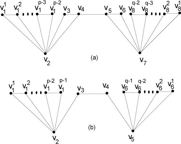
(a)C1(p, q) and (b)
(a)C2(p, q) and (b)
Let Ω1,n be the class of cacti other than stars such that each block of a cactus is an edge and Ω2,n be a class of cacti other than bundles such that at least one block of each cactus is an edge and at least one block is a cycle. Let Ωn be a class of cacti other than stars and bundles such that either all the blocks of a cactus are edges or a cactus has at least one block which is a cycle and at least one block which is an edge, i.e. Ωn = Ω1,n ∪ Ω2,n. Thus, we obatain
If ϕ′ : V(Γ) → {Xi : 1 ≤ i ≤ n} is a 1-1 map such that ϕ′(ui) = Xi for each ui ∈ V(Γ) then it is said to be defined on the graph Γ. The eigenvector X of A(Γ) is naturally defined on V(Γ). Thus, we have
The eigenequation for each v ∈ V(Γ) is
where all adjacent to v are in NΓ(v). If X ∈ Rn is an arbitrary unit vector, we have
where equality holds iff X is a FEv. If Γc is complement of Γ, then A(Γc) = J – I – A(Γ) with J and I as all-ones and identity matrix respectively. Thus, for X ∈ Rn
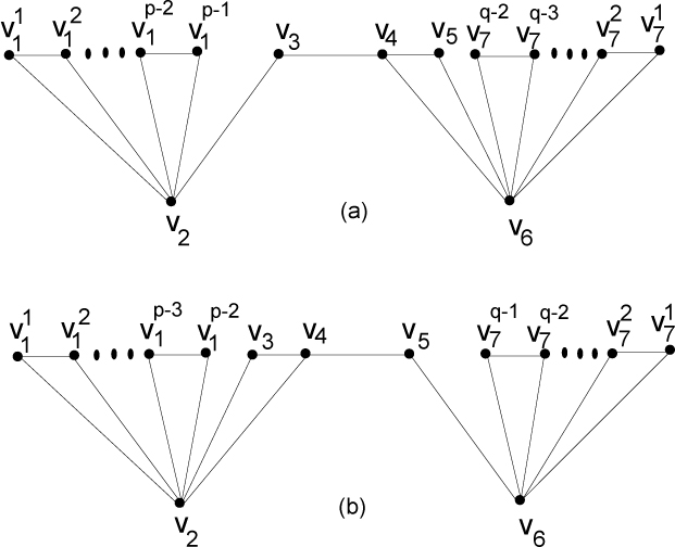
Let Y1 be FEv of C1(p, q)c which is defined on it. By (2.2), the vertices
Take Y1 = (X1, X2, X3, X4, X5, X6, X7, X8)T then the matrix equation is (A – λ1I)Y1 = 0 and
with least root λ1.
Let
Take
with least root
Let Y2 be FEv of C2(p, q)c. By (2.2), the vertices
Take Y2 = (X1, X2, X3, X4, X5, X6, X7)T then the matrix equation is (A – λ2 I)Y2 = 0 and
with least root λ2.
Let
Take
with least root
3 Minimizing graphs
Now, we present some important lemmas of the minimizing graph which are frequently used in next section. The classes of cacti which have graphs of even order are discussed from Lemma 3.1 to Lemma 3.6. Moreover, the cacti of odd order are studied from Lemma 3.7 to Lemma 3.10.
Firstly, we discuss the classes of cacti which have graphs of even order.
Lemma 3.1
Suppose that p, q ≥ 4, n ≥ 12 are integers with p, q, n ≡ 0(mod 2). If p > q + 2, then
where p + q + 2 = n = |V(C1(p – 2, q + 2)c)| = |V(C1(p, q)c)|.
Proof
From equation (2.5), we have f1(–3, p, q) = 325 – 17(p + q) – 35pq. Since for p, q ≥ 4 f1(–3, p, q) < 0. Therefore, least root of f1(λ, p, q) is λ1 < –3. Moreover, f1(λ, p – 2, q + 2) = (pq – 4q) + (16 – 4p – 4q)λ + (24 – 2p + 26q – 7pq)λ2 + (–56 + 18p + 10q + 2pq)λ3 + (–48 + 5p – 23q + 7pq)λ4 + (16 – 12p – 20q + 2pq)λ5 + (24 – 7p – 7q)λ6 + (8 – p – q)λ7 + λ8, and
As p is greater than q + 2 and λ is less than –3 therefore f1(λ, p, q)- f1(λ, p – 2, q + 2) > 0. Also, f1(–3, p – 2, q + 2) < 0 which implies that λmin(C1(p – 2, q + 2)c) < λmin(C1(p, q)c).
Corollary 3.2
Suppose that p, q ≥ 4, n ≥ 12 are integers with p, q, n ≡ 0(mod 2). If q > p + 2, then λmin(C1(p + 2, q – 2)c) < λmin(C1(p, q)c), where p + q + 2 = n.
Proof
Since, C1(p, q)c ≅ C1(q, p)c, therefore proof is same as of Lemma 3.1.
Lemma 3.3
Suppose that p, q ≥ 4 are integers with p, q ≡ 0(mod 2) and p + q + 2 = n =
where equality holds iff p =
Proof
When n ≡ 2(mod 4), then for p =
Now, by Lemma 3.1, if q + 2 < p and λ < –3, then λmin(C1(p – 2, q + 2)c) < λmin(C1(p, q)c) and by Corollary 3.1, if q > p + 2 and λ < –3, then λmin(C1(p + 2, q – 2)c) < λmin(C1(p, q)c).
Consequently, for n ≥ 14 and n ≡ 2(mod 4), we have
Lemma 3.4
Suppose that p ≥ 5, q ≥ 3, n ≥ 12 are integers with p, q ≡ 1(mod 2) and n ≡ 0(mod 2). If p > q + 2, then
where p + q + 2 = n is cardinality of both the cacti.
Proof
By (2.8),
Since p is greater than q + 2 and λ is less than –3,
Corollary 3.5
Suppose that p ≥ 3, q ≥ 5, n ≥ 12 are integers with p, q ≡ 1(mod 2) and n ≡ 0(mod 2). If q > p + 2, then λmin(
Proof
Since,
Lemma 3.6
Suppose that p, q ≥ 3 are integers with p, q ≡ 1(mod 2) and p + q + 2 = n =
where equality holds iff p =
Proof
When n ≡ 2(mod 4), then for p =
Now, by Lemma 3.4, for p > q + 2 and λ < –3, λmin(
Consequently, for n ≥ 14 and n ≡ 2(mod 4), we have
Now, we discuss the classes of graphs having graphs of odd order.
Lemma 3.7
Suppose that p ≥ 5, q ≥ 2 and n ≥ 13 are integers with p, n ≡ 1(mod 2) and q ≡ 0(mod 2). If p > q + 3, then
where p + q + 2 = n = |V(C2(p – 2, q + 2)c)| = |V(C2(p, q)c)|.
Proof
From equation (2.10), we have f2(–3, p, q) = 117 – (p + q) – 28q(p – 1). Since, for p ≥ 5 and q ≥ 2 f2(–3, p, q) < 0. Therefore, least root of f2(λ, p, q) is λ2 < –3. Also, f2(λ, p – 2, q + 2) = +(5q – pq) + (–20 + 4p – 8q + 3pq)λ + (16 – 8p – 15q + pq)λ2 + (39 – 7p + 11q – 5pq)λ3 + (–1 + 7p + 15q – 2pq) λ4 + (–17 + 6p + 6q)λ5 + (–7 + p + q)λ6 – λ7, and
where
If p – q → 4, then
Lemma 3.8
Suppose that p ≥ 4, q ≥ 3 and n ≥ 13 are integers with q, n ≡ 1(mod 2) and p ≡ 0(mod 2). If p > q + 3, then
where p + q + 2 = n.
Proof
From equation (2.12), we have
and
Thus, for p > q and λ < –3, we have
Corollary 3.9
Suppose that p ≥ 3, q ≥ 4 and n ≥ 13 are integers with p, n ≡ 1(mod 2) and q ≡ 0(mod 2). If q > p + 3, then λmin(C2(p + 2, q – 2)c) < λmin(C2(p, q)c), where p + q + 2 = n.
Proof
Using Lemma 3.8, if r > s + 3 and r + s + 2 = n then
Therefore, for n ≡ 1(mod 4), we have
Similarly for n ≡ 3(mod 4), we have
Now, by definition, for n ≡ 1(mod 4),
Consequently, λmin(C2(p + 2, q – 2)c) < λmin(C2(p, q)c) for q > p, which complete the proof.
Lemma 3.10
Suppose that p ≥ 3 and q ≥ 2 are integers with p ≡ 1(mod 2) and q ≡ 0(mod 2), where p + q + 2 = n is of the cacti. Then
where equality holds iff p =
Proof
When n ≡ 1(mod 4), then for p =
Now, by Lemma 3.7, if p is greater than q + 3 and λ is less than –3, then λmin(C2(p – 2, q + 2)c) < λmin(C2(p, q)c) and by Corollary 3.9, if q > p, q – p ≠ 2 and λ < –3, then λmin(C2(p + 2, q – 2)c) < λmin(C2(p, q)c).
Consequently, for n ≥ 13 and n ≡ 1(mod 4), we have
4 Characterization
This section includes the main results in which minimizing graphs are characterized in the family of connected graphs with the condition that the complement of each graph is a cactus such that either its each block is only an edge or it has at least one block which is an edge and at least one block which is a cycle. In Lemma 4.1 and 4.2, the basic results are developed which are used in the main results. In Lemma 4.3 and Lemma 4.4, minimizing graphs are characterized in
Lemma 4.1
Let n ≥ 12 and X = (X1, X2, X3, …, Xn)T be a real vector defined on C ∈ Ωn such that |X1| ≥ |X2| ≥ |X3| ≥ ... ≥ |Xn| and all Xi are either non-negative or non-positive. Then
where equality holds if C ≅ B1(n – 1) and C ≅ B2(n – 1) respectively.
Proof
Suppose that X is non-negative and discuss the following two cases:
Suppose that C ∈ Ωn is a cactus graph such that its each block is an edge i.e. C ∈ Ω1,n. Let X1 be the value of the vertex v ∈ C assigned by X. As n ≥ 10 and is not a bundle, therefore there exist a vertex in C say u which is not adjacent to v. Thus, a vertex w adjacent to u (w ∼ u) exists on a path from v to u as C is connected. A new cactus C̃ having each block as an edge can be found on the deletion of the edge wu and addition of vu in C. We find a star K1,n–1 with center v by repeating the same process for the non-neighbor of v in the cactus C̃ and so on. Thus, we have
Suppose that C ∈ Ωn is a cactus graph such that it has at least one block which is an edge and at least one block which is a cycle i.e. C ∈ Ω2,n. Assume that k is number of cycles in C, then
where vr, vr+1, vs, vs+1, …, vt, vt+1 are 2k distinct vertices of C. Moreover, the inequality in (4.1) does not disturb, if we add k terms (Xvr1 Xvr1+1 + Xvr2 Xvr2+1 +, …, + Xvrk Xvrk+1) in its right hand side. Consequently, from both the cases, we have
Assume n ≡ 1(mod 2). Since, in K1,n–1, one vertex, say v1 with d(v1) = n – 1 has value X1 and remaining n – 1 pendent vertices have values Xi for 2 ≤ i ≤ n. Pairing the vertices of degree 1 and joining each pair by an edge, we have
Assume n ≡ 0(mod 2). Since, in K1,n–1, one vertex, say v1 with d(v1) = n – 1 has value X1 and remaining n – 1 pendent vertices have values Xi for 2 ≤ i ≤ n. Pairing the n – 2 vertices of degree 1 and joining each pair by an edge, we have
So, (4.2) takes form
Lemma 4.2
For n ≥ 12 and Cc ∈
Proof
Assume that there is a unique vertex v ∈ Cc having positive value labeled by X. The degree of v in Cc is non-zero, i.e dCc(v) ≠ 0. As, if dCc(v) = 0, then C is a bundle, which is a contradiction to the construction of
Lemma 4.3
Suppose that C is a cactus graph such that Cc ∈
If n ≡ 0(mod 2), then either λmin(C1(p, q)c) ≤ λmin(Cc), or λmin(
If n ≡ 1(mod 2), then λmin(C2(p, q)c) ≤ λmin(Cc) with equality if C ≅ C2(p, q).
Proof
Assume X is a unit first eigenvector of Cc. Define V+ = {v : Xv ≥ 0, v ∈ V(Cc)} and V– = {v : Xv < 0, v ∈ V(Cc)} such that |V+|, |V–| ≥ 2 by Lemma 4.2. Suppose that the subgraphs C+ and C– of C are induced by the vertex sets V+ and V– respectively and E′ ≠ Φ is subset of E(C) with one end in C+ and other in C–. Thus, we have
Assume that n ≡ 0(mod 2), where n = p + q + 2. Let C̄ be a graph obtained from C by some possible addition or deletion of edges in C+ and C– such that the subgraph C̄+ and C̄– of C̄ induced by C+ and C– are cactus graphs satisfying one of the following possibilities, (i) each block of one of the subgraphs C̄+ and C̄– is an edge and other has at least one block which is a cycle and at least one block which is an edge, (ii) all the blocks of both the subgraphs C̄+ and C̄– are cycles, (iii) all the blocks of one subgraph are edges and of other are cycles, (iv) each block of one of the subgraphs C̄+ and C̄– is a cycle and other has at least one block which is a cycle and at least one block which is an edge, and (v) both the subgraphs C̄+ and C̄– have at least one block which is a cycle and at least one block which is an edge.
For (i), suppose C̄+ is a cactus such that its each block is an edge, otherwise we take –X as a first eigenvector. Let u′ be a vertex of C̄+ with maximum modulus among all the vertices, then by discussion of equation (4.1) in Lemma 4.1, we obtain a cactus with each block as an edge which is infect a star K1,p. Similarly, suppose that v′ is a vertex with maximum modulus among all the vertices of C̄–. Firstly, we delete an edge in each block such that no two deleted edges of any two blocks have a common vertex in C̄– and the deleted edge in a block which has v′ is not incident on this vertex. Thus, we obtain a subgraph of C̄– such that its each block is an edge. Then by the same discussion as of equation (4.2) in Lemma 4.1, we obtain a cactus with at least one block as a cycle and at least one block as an edge which is infect a star K1,q with edges among the pendent vertices having different end points.
Since n ≡ 0(mod 2) and n = p + q + 2, where n = |V+ ∪ V–| = |C̄+ ∪ C̄–|, p + 1 = |V+| = |C̄+| and q + 1 = |V–| = |C̄–|. Therefore, either both p and q are even or odd.
Suppose p and q both are even. By pairing the pendent vertices of the star K1,p which is obtained from C̄+ and joining them by edges, we have a bundle B1(p) with center u′ having maximum modulus value, where p + 1 = |V+| ≥ 3 is odd. Similarly, pair the remaining possible pendent vertices of the subgraph obtained from C̄– and join them by edges. Thus, we obtain a bundle B1(q) with center v′ having maximum modulus value, where q + 1 = |V+| ≥ 3 is odd. Thus, by Lemma 4.1 (a), we have
and
Suppose p and q both are odd. By pairing the pendent vertices of the star which is obtained from C̄+ and joining them by edges, we have a bundle B2(p) with center u′ having maximum modulus value, where p + 1 = |V+| ≥ 4 is even. Similarly, pair the remaining possible pendent vertices of the subgraph obtained from C̄– and join them by edges. Thus, we obtain a bundle B2(q) with center v′ having maximum modulus value, where q + 1 = |V+| ≥ 4 is even. Thus, by Lemma 4.1 (b), we have
Assume that u″ ∈ C̄+ and v″ ∈ C̄– have minimum modulus values. Then
Using (4.4), (4.5), (4.8) and (4.6), (4.7), (4.8) in (4.3) respectively, we have
Since p ≥ q ≥ 2. Therefore, if we take u″ ∈ B1(p), v″ ∈ B1(q) of degree 2 and u″ ∈ B2(p), v″ ∈ B2(q) of degree 1. Then (4.9) and (4.10) becomes,
Now by the equations (2.1)-(2.4) and (4.11), we have λmin(Cc) = XTA(Cc)X = XT(J – I – A(C))X = XT(J – I)X – XTA(C)X ≥ XT(J – I)X – XTA(C1(p, q))X = XTA(C1(p, q)c)X ≥ λmin(C1(p, q)c) ⇒ λmin(C1(p, q)c) ≤ λmin(Cc). Similarly by equations (2.1)-(2.4) and (4.12), we have λmin(
Thus, for n ≡ 0(mod 2), either λmin(C1(p, q)c) ≤ λmin(Cc) or λmin(
Assume that n ≡ 1(mod 2), where n = p + q + 2. Let C̄ be a graph obtained from C with subgraph C̄+ and C̄– induced from C+ and C– are cactus graphs satisfying any one of the possibilities which are stated in (a). For (i), we proceed same as in (a) and find the cactus graphs which are infect stars with some possible edges among the pendent vertices having different end points from both the subgraphs C̄+ and C̄– after the deletion and addition of some edges. Since n ≡ 1(mod 2) and n = p + q + 2, where n = |V+ ∪ V–| = |C̄+ ∪ C̄–|, p + 1 = |V+| = |C̄+| and q + 1 = |V–| = |C̄–|. Therefore, either p is even and q is odd or vice versa. Without loss of generality, we assume p as odd and q even.
Suppose that u′ and u″ in C̄+, and v′ and v″ in C̄– have have maximum and minimum modulus values respectively. Then by the same discussion as in (a) with the help of Lemma 4.1, we have
and
where the bundle B2(p) has center u′ with maximum modulus value and p + 1 = |V+| ≥ 4 is even. Similarly, the bundle B1(q) has center v′, with maximum modulus value and q + 1 = |V+| ≥ 3 is odd. Now, using (4.13), (4.14) and (4.15) in (4.3), we have
Since p, q ≥ 2. Therefore, if we take u″ ∈ B2(p) and v″ ∈ B1(p) such that degree of u″ in B2(p) is 1 and degree of v″ in B1(q) is 2. Thus, (4.16) becomes
Now by the equations (2.1)-(2.4) and (4.17), λmin(C2(p, q)c) ≤ λmin(Cc), where n = p + q + 2 > 10 and n ≡ 1(mod 2). Similarly, it also can be prove for all other possibilities.
Now finally we prove that there does not exist any vertex in V+ such that its value given by X is zero and E′ has exactly one edge. Firstly, among the vertices of C1(p, q), we prove that v2 = u′ and v4 = u″ are unique ones in C+ and, v5 = v″ and v7 = v′ are unique ones in C– with maximum and minimum modulus, respectively. For this, we will show 0 ≤ X4 < X3 < X1 < X2 and X7 < X8 < X6 < X5 < 0. By Lemma 4.2, we have X1, X2, X3 non negative and X4, X5, X6, X7, X8 negative values in the first eigenvector X of C1(p, q)c. By (2.5), λ1(X2 – X1) = –(p – 4)X1 – X3 – X4 < 0, (λ1 + 1)(X1 – X3) = –(X1 – X4) < 0, and λ1(X3 – X4) = X5 < 0 ⇒ X2 – X1 > 0, X1 – X3 > 0 and X3 – X4 > 0. Thus
Similarly, λ1(X8 – X7) = X5 + X6 + (q – 4)X8 < 0, (λ1 + 1)(X6 – X8) = –X5 + X8 < 0 and λ1(X5 – X6) = –X4 < 0 ⇒ X8 – X7 > 0, X5 – X6 > 0 and X6 – X8 > 0. Thus
If any one of the vertices v1, v2 and v3 has value zero assigned by X, then by (4.18) X3 = 0 = X4. Moreover, by (2.5), we have X5 = 0 = X6, which is a contradiction to the construction of V– and C–. If the value of the vertex v4 labeled by X is zero, then by (2.5), λ1(X5 – X6) = 0 ⇒ X5 = X6 which is a contradiction to (4.19) (i.e. X5 is a unique one in C–). Consequently, X1, X2, X3 and X4 are non zero positive values of X. Thus, v ∉ V+ such that Xv = 0. By (4.4), (4.5), (4.8), (4.9) and the above discussion, we have C+ = C̄+ = B1(p), C– = C̄– = B1(q) and E′ has only one edge u″v″ = v4v5 in B1(p, q). Similarly, we can prove for
Similarly, we can prove the following result:
Lemma 4.4
Suppose that C is a cactus graph of order n = p + q + 2 ≥ 10 such that Cc ∈
If n ≡ 0(mod 2), then either λmin(C1(p, q)c) < λmin(Cc) or λmin(
If n ≡ 1(mod 2), then λmin(C2(p, q)c) < λmin(Cc).
Theorem 4.5
Suppose that C is a cactus graph of order n such that
Assume that n ≡ 0(mod 2), p, q ≥ 4 and n = p + q + 2:
For p, q ≡ 0(mod 2);
If n ≥ 14 and n ≡ 2(mod 4), then
If n ≥ 12 and n ≡ 0(mod 4), then
For p, q ≡ 1(mod 2);
If n ≥ 14 and n ≡ 2(mod 4), then
If n ≥ 12 and n ≡ 0(mod 4), then
Assume that n ≡ 1(mod 2), p ≡ 1(mod 2) and q ≡ 0(mod 2):
If n ≥ 13 and n ≡ 1(mod 4), then
If n ≥ 15 and n ≡ 3(mod 4), then λmin
5 Conclusions
Petrović et al. [23] explored a unique cactus as a minimizing graph from the class of cacti such that the order of each cactus is n. But, it is noted that the complement of the proposed minimizing graph is disconnected. In this paper, we characterize the minimizing graphs in a collection of connected graphs such that the complement of each graph of order n is a cactus with the condition that either its each block is only an edge or it has at least one block which is an edge and at least one block which is a cycle. However, the problem is still open to characterize the minimizing graphs in a collection of connected graphs whose complements are in the complete class of cacti (each block of a cactus is only an edge, at least one block is an edge and at least one block is a cycle, or each block is a cycle).
Acknowledgement
The authors are indebted to the anonymous referee for his valuable comments to improve the original version of this paper. The first author is supported by NSFC of China (No.11701530) and the Fundamental Research Funds for the Central Universities (No.2652017146).
References
[1] Collatz L., Sinogowitz U., Spektren endlicher Grafen, Abhandlungen aus dem Mathematischen Seminar der Universität Hamburg, 1957, 21, 63-77.10.1007/BF02941924Search in Google Scholar
[2] Cvetković D., Rowlinson P., The largest eigenvalues of a graph: a survey, Linear Multileaner Algebra, 1990, 28, 3-33.10.1080/03081089008818026Search in Google Scholar
[3] Cvetković D., Doob M., Sachs H., Spectra of Graphs, 3rd ed. Johann Ambrosius Barth, Heidelberg, 1995.Search in Google Scholar
[4] Cvetković D., Rowlinson P., Simić S., Spectral Generalizations of Line Graphs: on Graph with Least Eigenvalue –2, Cambridge Uni. Press, London Math. Soc., 2014.Search in Google Scholar
[5] Hong Y., Shu J., Sharp lower bounds of the least eigenvalue of planar graphs, Linear Algebra Appl., 1999, 296, 227-232.10.1016/S0024-3795(99)00129-9Search in Google Scholar
[6] Bell F.K., Cvetković D., Rowlinson P., Simić S., Graph for which the least eigenvalues is minimal, II, Linear Algebra Appl., 2008, 429, 2168-2179.10.1016/j.laa.2008.06.018Search in Google Scholar
[7] Du Z., Spectral properties of a class of unicyclic graphs, J. Inequal. Appl., 2017, Article number: 9610.1186/s13660-017-1367-2Search in Google Scholar PubMed PubMed Central
[8] Guan M., Zhai M., Wu Y., On the sum of two largest Laplacian eigenvalue of trees, J. Inequal. Appl., 2014, Article number: 242.10.1186/1029-242X-2014-242Search in Google Scholar
[9] Guo S.-G., Liu X., Zhang R., Yu G., Ordering non-bipartite unicyclic graphs with pendant vertices by the least Q – eigenvalue, J. Inequal. Appl., 2016, 2016: 136.10.1186/s13660-016-1077-1Search in Google Scholar
[10] Petrović M., Borovićanin B., Aleksić T., Bicyclic graphs for which the least eigenvalue is minimum, Linear Algebra Appl., 2009, 430, 1328-1335.10.1016/j.laa.2008.10.026Search in Google Scholar
[11] Petrović M., Aleksić T., Simić S., Further results on the least eigenvalue of connected graphs, Linear Algebra Appl., 2011, 435, 2303-2313.10.1016/j.laa.2011.04.030Search in Google Scholar
[12] Zheng Y., Chang A., Li J., Rula S., Bicyclic graphs with maximum sum of the two largest Laplacian eigenvalues, J. Inequal. Appl., 2016, Article number: 287.10.1186/s13660-016-1235-5Search in Google Scholar
[13] Zheng Y., Chang A., Li J., On the sum of two largest Laplacian eigenvalue of unicyclic graphs, J. Inequal. Appl., 2015, Article number: 275.10.1186/s13660-015-0794-1Search in Google Scholar
[14] Bell F.K., Cvetković D., Rowlinson P., Simić S., Graph for which the least eigenvalues is minimal, I, Linear Algebra Appl., 2008, 429, 234-241.10.1016/j.laa.2008.02.032Search in Google Scholar
[15] Fan Y.-Z., Zhang F.-F., Wang Y., The least eigenvalue of the complements of trees, Linear Algebra Appl., 2011, 435, 2150-2155.10.1016/j.laa.2011.04.011Search in Google Scholar
[16] Javaid M., Minimizing graph of the connected graphs whose complements are bicyclic with two cycles, Turk. J. Math., 2017, 41, 1433-1445.10.3906/mat-1608-6Search in Google Scholar
[17] Javaid M., Characterization of the minimizing graph of the connected graphs whose complements are bicyclic, Mathematics, 2017, 5, 18, 10.3390/math5010018.Search in Google Scholar
[18] Wang Y., Fan Y.-Z., Li X.-X., Zhang F.-F., The least eigenvalue of graphs whose complements are unicyclic, Discuss. Math. Graph Theory, 2015, 35(2), 249-260.10.7151/dmgt.1796Search in Google Scholar
[19] Javaid M., On the second minimizing graph in the set of complements of trees, AKCE Int. J. Graphs Comb., 2018, https://doi.org/10.1016/j.akcej.2018.11.005.10.1016/j.akcej.2018.11.005Search in Google Scholar
[20] Sudhakar S., Francis S., Balaji V., Odd mean labeling for two star graph, Appl. Math. Nonlinear Sci., 2017, 2(1), 195-200.10.21042/AMNS.2017.1.00016Search in Google Scholar
[21] Basavanagoud B., Desai V.R., Patil S., (β, α)-connectivity index of graphs, Appl. Math. Nonlinear Sci., 2017, 2(1), 21-30.10.21042/AMNS.2017.1.00003Search in Google Scholar
[22] Zhou S., Xu L., Xu Y., A sufficient condition for the existence of a k – factor excluding a given r – factor, Appl. Math. Nonlinear Sci., 2017, 2(1), 13-20.10.21042/AMNS.2017.1.00002Search in Google Scholar
[23] Petrović M., Aleksić T., Simić S., On the least eigenvalue of cacti, Linear Algebra Appl., 2011, 435, 2357-2364.10.1016/j.laa.2011.02.011Search in Google Scholar
© 2019 Wang et al., published by De Gruyter
This work is licensed under the Creative Commons Attribution 4.0 Public License.
Articles in the same Issue
- Regular Articles
- On the Gevrey ultradifferentiability of weak solutions of an abstract evolution equation with a scalar type spectral operator of orders less than one
- Centralizers of automorphisms permuting free generators
- Extreme points and support points of conformal mappings
- Arithmetical properties of double Möbius-Bernoulli numbers
- The product of quasi-ideal refined generalised quasi-adequate transversals
- Characterizations of the Solution Sets of Generalized Convex Fuzzy Optimization Problem
- Augmented, free and tensor generalized digroups
- Time-dependent attractor of wave equations with nonlinear damping and linear memory
- A new smoothing method for solving nonlinear complementarity problems
- Almost periodic solution of a discrete competitive system with delays and feedback controls
- On a problem of Hasse and Ramachandra
- Hopf bifurcation and stability in a Beddington-DeAngelis predator-prey model with stage structure for predator and time delay incorporating prey refuge
- A note on the formulas for the Drazin inverse of the sum of two matrices
- Completeness theorem for probability models with finitely many valued measure
- Periodic solution for ϕ-Laplacian neutral differential equation
- Asymptotic orbital shadowing property for diffeomorphisms
- Modular equations of a continued fraction of order six
- Solutions with concentration and cavitation to the Riemann problem for the isentropic relativistic Euler system for the extended Chaplygin gas
- Stability Problems and Analytical Integration for the Clebsch’s System
- Topological Indices of Para-line Graphs of V-Phenylenic Nanostructures
- On split Lie color triple systems
- Triangular Surface Patch Based on Bivariate Meyer-König-Zeller Operator
- Generators for maximal subgroups of Conway group Co1
- Positivity preserving operator splitting nonstandard finite difference methods for SEIR reaction diffusion model
- Characterizations of Convex spaces and Anti-matroids via Derived Operators
- On Partitions and Arf Semigroups
- Arithmetic properties for Andrews’ (48,6)- and (48,18)-singular overpartitions
- A concise proof to the spectral and nuclear norm bounds through tensor partitions
- A categorical approach to abstract convex spaces and interval spaces
- Dynamics of two-species delayed competitive stage-structured model described by differential-difference equations
- Parity results for broken 11-diamond partitions
- A new fourth power mean of two-term exponential sums
- The new operations on complete ideals
- Soft covering based rough graphs and corresponding decision making
- Complete convergence for arrays of ratios of order statistics
- Sufficient and necessary conditions of convergence for ρ͠ mixing random variables
- Attractors of dynamical systems in locally compact spaces
- Random attractors for stochastic retarded strongly damped wave equations with additive noise on bounded domains
- Statistical approximation properties of λ-Bernstein operators based on q-integers
- An investigation of fractional Bagley-Torvik equation
- Pentavalent arc-transitive Cayley graphs on Frobenius groups with soluble vertex stabilizer
- On the hybrid power mean of two kind different trigonometric sums
- Embedding of Supplementary Results in Strong EMT Valuations and Strength
- On Diophantine approximation by unlike powers of primes
- A General Version of the Nullstellensatz for Arbitrary Fields
- A new representation of α-openness, α-continuity, α-irresoluteness, and α-compactness in L-fuzzy pretopological spaces
- Random Polygons and Estimations of π
- The optimal pebbling of spindle graphs
- MBJ-neutrosophic ideals of BCK/BCI-algebras
- A note on the structure of a finite group G having a subgroup H maximal in 〈H, Hg〉
- A fuzzy multi-objective linear programming with interval-typed triangular fuzzy numbers
- Variational-like inequalities for n-dimensional fuzzy-vector-valued functions and fuzzy optimization
- Stability property of the prey free equilibrium point
- Rayleigh-Ritz Majorization Error Bounds for the Linear Response Eigenvalue Problem
- Hyper-Wiener indices of polyphenyl chains and polyphenyl spiders
- Razumikhin-type theorem on time-changed stochastic functional differential equations with Markovian switching
- Fixed Points of Meromorphic Functions and Their Higher Order Differences and Shifts
- Properties and Inference for a New Class of Generalized Rayleigh Distributions with an Application
- Nonfragile observer-based guaranteed cost finite-time control of discrete-time positive impulsive switched systems
- Empirical likelihood confidence regions of the parameters in a partially single-index varying-coefficient model
- Algebraic loop structures on algebra comultiplications
- Two weight estimates for a class of (p, q) type sublinear operators and their commutators
- Dynamic of a nonautonomous two-species impulsive competitive system with infinite delays
- 2-closures of primitive permutation groups of holomorph type
- Monotonicity properties and inequalities related to generalized Grötzsch ring functions
- Variation inequalities related to Schrödinger operators on weighted Morrey spaces
- Research on cooperation strategy between government and green supply chain based on differential game
- Extinction of a two species competitive stage-structured system with the effect of toxic substance and harvesting
- *-Ricci soliton on (κ, μ)′-almost Kenmotsu manifolds
- Some improved bounds on two energy-like invariants of some derived graphs
- Pricing under dynamic risk measures
- Finite groups with star-free noncyclic graphs
- A degree approach to relationship among fuzzy convex structures, fuzzy closure systems and fuzzy Alexandrov topologies
- S-shaped connected component of radial positive solutions for a prescribed mean curvature problem in an annular domain
- On Diophantine equations involving Lucas sequences
- A new way to represent functions as series
- Stability and Hopf bifurcation periodic orbits in delay coupled Lotka-Volterra ring system
- Some remarks on a pair of seemingly unrelated regression models
- Lyapunov stable homoclinic classes for smooth vector fields
- Stabilizers in EQ-algebras
- The properties of solutions for several types of Painlevé equations concerning fixed-points, zeros and poles
- Spectrum perturbations of compact operators in a Banach space
- The non-commuting graph of a non-central hypergroup
- Lie symmetry analysis and conservation law for the equation arising from higher order Broer-Kaup equation
- Positive solutions of the discrete Dirichlet problem involving the mean curvature operator
- Dislocated quasi cone b-metric space over Banach algebra and contraction principles with application to functional equations
- On the Gevrey ultradifferentiability of weak solutions of an abstract evolution equation with a scalar type spectral operator on the open semi-axis
- Differential polynomials of L-functions with truncated shared values
- Exclusion sets in the S-type eigenvalue localization sets for tensors
- Continuous linear operators on Orlicz-Bochner spaces
- Non-trivial solutions for Schrödinger-Poisson systems involving critical nonlocal term and potential vanishing at infinity
- Characterizations of Benson proper efficiency of set-valued optimization in real linear spaces
- A quantitative obstruction to collapsing surfaces
- Dynamic behaviors of a Lotka-Volterra type predator-prey system with Allee effect on the predator species and density dependent birth rate on the prey species
- Coexistence for a kind of stochastic three-species competitive models
- Algebraic and qualitative remarks about the family yy′ = (αxm+k–1 + βxm–k–1)y + γx2m–2k–1
- On the two-term exponential sums and character sums of polynomials
- F-biharmonic maps into general Riemannian manifolds
- Embeddings of harmonic mixed norm spaces on smoothly bounded domains in ℝn
- Asymptotic behavior for non-autonomous stochastic plate equation on unbounded domains
- Power graphs and exchange property for resolving sets
- On nearly Hurewicz spaces
- Least eigenvalue of the connected graphs whose complements are cacti
- Determinants of two kinds of matrices whose elements involve sine functions
- A characterization of translational hulls of a strongly right type B semigroup
- Common fixed point results for two families of multivalued A–dominated contractive mappings on closed ball with applications
- Lp estimates for maximal functions along surfaces of revolution on product spaces
- Path-induced closure operators on graphs for defining digital Jordan surfaces
- Irreducible modules with highest weight vectors over modular Witt and special Lie superalgebras
- Existence of periodic solutions with prescribed minimal period of a 2nth-order discrete system
- Injective hulls of many-sorted ordered algebras
- Random uniform exponential attractor for stochastic non-autonomous reaction-diffusion equation with multiplicative noise in ℝ3
- Global properties of virus dynamics with B-cell impairment
- The monotonicity of ratios involving arc tangent function with applications
- A family of Cantorvals
- An asymptotic property of branching-type overloaded polling networks
- Almost periodic solutions of a commensalism system with Michaelis-Menten type harvesting on time scales
- Explicit order 3/2 Runge-Kutta method for numerical solutions of stochastic differential equations by using Itô-Taylor expansion
- L-fuzzy ideals and L-fuzzy subalgebras of Novikov algebras
- L-topological-convex spaces generated by L-convex bases
- An optimal fourth-order family of modified Cauchy methods for finding solutions of nonlinear equations and their dynamical behavior
- New error bounds for linear complementarity problems of Σ-SDD matrices and SB-matrices
- Hankel determinant of order three for familiar subsets of analytic functions related with sine function
- On some automorphic properties of Galois traces of class invariants from generalized Weber functions of level 5
- Results on existence for generalized nD Navier-Stokes equations
- Regular Banach space net and abstract-valued Orlicz space of range-varying type
- Some properties of pre-quasi operator ideal of type generalized Cesáro sequence space defined by weighted means
- On a new convergence in topological spaces
- On a fixed point theorem with application to functional equations
- Coupled system of a fractional order differential equations with weighted initial conditions
- Rough quotient in topological rough sets
- Split Hausdorff internal topologies on posets
- A preconditioned AOR iterative scheme for systems of linear equations with L-matrics
- New handy and accurate approximation for the Gaussian integrals with applications to science and engineering
- Special Issue on Graph Theory (GWGT 2019)
- The general position problem and strong resolving graphs
- Connected domination game played on Cartesian products
- On minimum algebraic connectivity of graphs whose complements are bicyclic
- A novel method to construct NSSD molecular graphs