Solutions with concentration and cavitation to the Riemann problem for the isentropic relativistic Euler system for the extended Chaplygin gas

1 Introduction

It is very important to understand the relativistic fluid dynamics in the study of various astrophysical phenomena [1], such as the gravitational collapse, the supernova explosion and the formation and acceleration of the universe. Nowadays, there exists a vast amount of literature in various models of relativistic fluid dynamics since the fundamental work of Taub [2]. However, only a few analytical theories have been developed such as in [3, 4, 5, 6] due to the complicated structures of various relativistic fluid dynamics models. In this present work, we draw our attention on the isentropic Euler system of two conservation laws consisting of energy and momentum in special relativity in the following form [3, 5, 6, 7]

Here the unknown state variables ρ(x, t) and v(x, t) stand for the proper-energy density and the particle speed respectively and the unknown function p(ρ) is used to denote scalar pressure which is a function of ρ for the isentropic situation. In addition, the constant c is the speed of light. The system (1.1) was often used to describe the dynamics of plane waves in special relativistic fluids in the two-dimensional Minkowski space-time [3].

In our present study, the equation of state p(ρ) is chosen as the third-order form of the extended Chaplygin gas [8, 9] as follows:

in which A₁, A₂, A₃ ≥ 0 and B > 0. It requires that the speed of sound p′(ρ) is less than the speed of light c, such that the condition A₁ + 2A₂ρ + 3A₃ρ² + Bαρ^–α–1 < c² is satisfied. The Chaplygin gas with the equation of state given by p(ρ) = −Bρ with the constant B > 0 was first introduced by Chaplygin [10] as an effective mathematical approximation to compute the lifting force on a wing of an airplane. The equation of state for the Chaplygin gas is also very suitable to describe the dark energy and the dark matter in the universe within the framework of string theory [11]. In order to be consistent with the observed data, the equation of state was generalized to the form p(ρ) = – Bρα for the generalized Chaplygin gas [12] and subsequently was further modified to the form p(ρ) = Aρ – Bρα for the modified Chaplygin gas [13], in which A, B > 0 and 0 < α ≤ 1. It is essential to deal with a two fluid model about the equation of state for the modified Chaplygin gas for the reason that the first term Aρ gives an ordinary fluid obeying a linear barotropic equation of state while the second one – Bρα is the pressure to some power of the inverse of energy density. However, it is possible to consider the barotropic fluid, whose equation of state is quadratic and to even higher orders. In view of the aforementioned facts, the extended Chaplygin gas with the equation of state p(ρ)=Σk=1nAkρk−Bρα has been proposed by Pourhassan and Kahya [8]. It is easy to know that the extended Chaplygin gas recovers all the above Chaplygin gases by selecting A_k (k = 1, …, n) and α suitably. It is worthwhile to notice that the third-order form of the extended Chaplygin gas with the equation of state (1.2) has a good agreement with the cosmological parameters such as dark energy density, scale factor and Hubble expansion parameter [9, 14, 15, 16]. Of course we can also carry out the study for higher n terms of the extended Chaplygin gas, but the effects of more corrected terms are infinitesimal and are therefore of less importance [9]. Due to the above results, we shall draw our attention on the third-order form of the extended Chaplygin gas with the equation of state (1.2).

It is well known that the explicit solution can help us to understand the formation mechanism of singularities. For this purpose, we restrict ourselves to consider the system (1.1)-(1.2) with the Riemann-type initial data which is taken to be

Formally, if we adopt the Newtonian limit (namely the limit vc → 0 is taken), then the system (1.1)-(1.2) becomes the classical isentropic Euler system for the compressible fluid in the form

which has been widely studied as in [17, 18]. On the other hand, if the limit A₁, A₂, A₃, B → 0 is taken, then the system (1.1)-(1.2) turns out to be the following zero-pressure relativistic Euler system

The system (1.5) is a non-strictly hyperbolic and completely linearly degenerate system, whose elementary wave only involves the contact discontinuity. More specifically, the solution to the Riemann problem (1.3) and (1.5) is either a delta shock wave solution when v_– > v₊ or a two-contact-discontinuity solution with a vacuum state between them when v_– < v₊. It is worth mentioning that the evolution of universe is in agreement with the pressureless fluid of the dark matter era at the early stage and subsequently is also consistent with the cosmic fluid to mimic the cosmological constant of the dark energy era at the later stage [14]. Motivated by the above observation, it is of great interest to investigate the transition between the two different stages of the universe by studying the vanishing pressure limits of solutions to the Riemann problem (1.1)-(1.3) where A₁, A₂, A₃, B → 0 is taken.

The first task of this paper is to solve the Riemann problem for the isentropic relativistic Euler system (1.1) associated with the equation of state (1.2). It is easy to get that the system (1.1) associated with (1.2) is strictly hyperbolic and each of the two characteristic fields is genuinely nonlinear. As a consequence, the solutions to the Riemann problem (1.1)-(1.3) are four kinds of different combinations between 1-shock (or 1-rarefaction) wave and 2-shock (or 2-rarefaction) wave, which depends on the choice of initial Riemann data (1.3). The second task of this paper is to consider the limits A₁, A₂, A₃, B → 0 of solutions to the Riemann problem (1.1)-(1.3) as the pressure tends to zero. Our discussion should be divided into two parts: (1) c > v_– > v₊ > –c and (2) –c < v_– < v₊ < c according to the two different structures of the solutions to the Riemann problem (1.3) and (1.5). To be more precise, the phenomenon of concentration can be identified and analyzed for the case c > v_– > v₊ > –c, where the limit of solution consisting of two shock waves to the Riemann problem (1.1)-(1.3) tends to a δ-shock wave solution as A₁, A₂, A₃, B → 0 while the intermediate density between the two shock waves tends to be a weight Dirac δ-measure. In contrast, the phenomenon of cavitation can also be captured and observed for the case –c < v_– < v₊ < c, where the limit of the solution consisting of two rarefaction waves to the Riemann problem (1.1)-(1.3) tends to a two-contact-discontinuity solution with a vacuum state between them as A₁, A₂, A₃, B → 0 while the intermediate density between the two rarefaction waves tends to be zero (namely a vacuum state).

For the related work about the isentropic relativistic Euler system (1.1), the equation of state p(ρ) = k²ρ was first investigated by Smoller and Temple [3] where the global existence of BV weak solutions to the Cauchy problem for the system (1.1) was proved analytically by employing Glimm’s scheme. Furthermore, the Riemann problem for the system (1.1) with the equation of state given by a smooth function p(ρ) and then the Cauchy problem for the system (1.1) with the equation of state obeying the γ law were also considered in [5]. When the perturbation is arbitrarily large, the uniqueness of Riemann solution to the system (1.1) was established by Chen and Li [6] in the class of entropy solutions in L^∞ ∩ BV_loc by making use of the detailed analysis of the global behavior of shock wave curves in the half-upper (ρ, v) phase space. Li, Feng and Wang [7] made a step further to construct the global entropy solutions to the Cauchy problem for the system (1.1) with a class of large initial data including the interaction between shock waves and rarefaction waves.

The formation of vacuum state and delta shock wave to the Riemann problem for the zero-pressure gas dynamics system [19, 20] was considered initially for the isothermal case [21] with the equation of state given by p(ρ) = cρ and the isentropic case [22] with the equation of state given by p(ρ) = cρ^γ, 1 < γ < 3 by making use of the vanishing pressure limit approach. The result was further extended to the generalized zero-pressure gas dynamics system in [23]. Also see for the other related works [24, 25, 26, 27] and the references cited therein. It is worthwhile to notice that the limits of solutions to the Riemann problems from the various isentropic Chaplygin gas dynamic systems [28, 29, 30, 31, 32] to the zero-pressure gas dynamic system have also been widely investigated in a variety of contents [33, 34, 35, 36, 37, 38], which are not described in detail any more in the paper.

As for the formation of vacuum state and delta shock wave to the Riemann problem for the zero-pressure relativistic Euler system (1.5), Yin and Sheng first investigated the vanishing pressure limits of solutions to the Riemann problems about the Euler system of conservation laws consisting of energy and momentum in special relativity for the isothermal [39] and isentropic [40] situations, in which the phenomena of concentration and cavitation can be observed and analyzed in detail. Subsequently, Li and Shao [41] considered the vanishing pressure limits of solutions to the Riemann problem (1.1)-(1.3) for the isentropic relativistic Euler system for the generalized Chaplygin gas where A_i = 0 (i = 1, 2, 3) was taken in (1.2), in which the delta shock wave was also involved in the solution to the Riemann problem (1.1)-(1.3) for the generalized Chaplygin gas when A_i = 0 (i = 1, 2, 3) in (1.2). Yin and Sheng [42] made a step further to generalize the above results to the Euler system consisting of three conservation laws to describe baryon numbers, energy and momentum in special relativity. Furthermore, Yin and Song [43] considered the vanishing pressure limits of solutions to the Riemann problems about the Euler system of conservation laws consisting of baryon numbers and momentum in special relativity for the Chaplygin gas. In addition, Yang and Zhang [44] introduced the flux approximation approach to study the formation of vacuum state and delta shock wave to the Riemann problem for the zero-pressure relativistic Euler system (1.5).

The paper is arranged as follows. In Section 2, we are mainly concerned with the construction of solutions to the Riemann problems for the isentropic relativistic Euler system (1.1) associated with the equation of state (1.2) in detail. In addition, we give a brief description of the solutions to the Riemann problem for the zero-pressure relativistic Euler system (1.5). In Section 3, we shall focus on the vanishing pressure limits of solutions to the Riemann problems from the system (1.1)-(1.2) to the zero-pressure relativistic Euler system (1.5) for the case c > v_– > v₊ > –c when the limit A₁, A₂, A₃, B → 0 is taken, in which the formation of δ-shock wave can be observed and analyzed. In Section 4, we turn back to investigate the formation of vacuum state for the case –c < v_– < v₊ < c when the limit A₁, A₂, A₃, B → 0 is taken.

2 The Riemann problems for the isentropic and zero-pressure relativistic Euler systems

In this section, we first illustrate the solutions to the Riemann problem for the isentropic relativistic Euler system (1.1) associated with the equation of state (1.2). Then, we recollect the related results for the zero-pressure relativistic Euler system (1.5), whose Riemann solution is a delta shock wave solution when c > v_– > v₊ > –c or a two-contact-discontinuity solution with a vacuum state between them when –c < v_– < v₊ < c.

2.1 The Riemann problem for the system (1.1) with the equation of state (1.2)

In this subsection, we shall first analyze the properties of elementary waves and then construct the solutions to the Riemann problem (1.1)-(1.3) for all kinds of situations. Since the speed of sound p′(ρ) is less than the speed of light c, the condition A₁ + 2A₂ρ + 3A₃ρ² + Bαρ^–α–1 < c² has to hold. There exist ρ₁ and ρ₂ satisfying 0 < ρ₁ < ρ < ρ₂ < +∞ for the fixed A₁, A₂, A₃, B, in which ρ₁ and ρ₂ are determined by

A1+2A2ρ+3A3ρ2+Bαρ−α−1=c2. (2.1)

In fact, the above ρ₁ and ρ₂ can be calculated numerically when all the coefficients A₁, A₂, A₃, B and α are given. More precisely, we can estimate ρ₁ and ρ₂ simply for sufficiently small A₁, A₂, A₃, B. It can be concluded that the following two inequalities

Bαρ1−α−1<c2andA1+2A2ρ2+3A3ρ22<c2 (2.2)

hold simultaneously, which enables us to have at least

ρ1>(Bαc2)1α+1andρ2<A2+3A3(c2−A1)+A123A3. (2.3)

Thus, the physically relevant region of solutions for the fixed A₁, A₂, A₃, B is restricted to

V={(ρ,v):ρ1<ρ<ρ2, |v|<c}. (2.4)

In addition, it is easy to know from (2.1) that

limA1,A2,A3,B→0⁡ρ1=0andlimA1,A2,A3,B→0⁡ρ2=+∞. (2.5)

The system (1.1)-(1.2) can be rewritten in the following quasi-linear form

Cρvt+Dρvx=00, (2.6)

where the matrixes C and D are given respectively by

C=(A1+2A2ρ+3A3ρ2+αBρ−α−1)v2+c4c2(c2−v2)2v(A1ρ+A2ρ2+A3ρ3−Bρ−α+ρc2)(c2−v2)2(A1+2A2ρ+3A3ρ2+αBρ−α−1+c2)vc2−v2(A1ρ+A2ρ2+A3ρ3−Bρ−α+ρc2)(c2+v2)(c2−v2)2

and

D=(A1+2A2ρ+3A3ρ2+αBρ−α−1+c2)vc2−v2(A1ρ+A2ρ2+A3ρ3−Bρ−α+ρc2)(c2+v2)(c2−v2)2(A1+2A2ρ+3A3ρ2+αBρ−α−1+v2)c2c2−v22vc2(A1ρ+A2ρ2+A3ρ3−Bρ−α+ρc2)(c2−v2)2.

By means of a direct calculation, we can achieve two real and distinct eigenvalues

λ1(ρ,v)=c2(v−A1+2A2ρ+3A3ρ2+αBρ−α−1)c2−vA1+2A2ρ+3A3ρ2+αBρ−α−1<c2(v+A1+2A2ρ+3A3ρ2+αBρ−α−1)c2+vA1+2A2ρ+3A3ρ2+αBρ−α−1=λ2(ρ,v). (2.7)

Corresponding to each λ_i(i = 1, 2), the right eigenvectors are calculated respectively by

r1→=(−1c2−v2,A1+2A2ρ+3A3ρ2+αBρ−α−1A1ρ+A2ρ2+A3ρ3−Bρ−α+ρc2)T,r2→=(1c2−v2,A1+2A2ρ+3A3ρ2+αBρ−α−1A1ρ+A2ρ2+A3ρ3−Bρ−α+ρc2)T. (2.8)

Thus the system (1.1)-(1.2) is strictly hyperbolic [3, 6, 46]. Let us introduce the notion ∇=(∂∂ρ,∂∂v), by a direct calculation, then we have

∂λ1(ρ,v)∂ρ=c2[2A2+6A3ρ−α(α+1)Bρ−α−2](v2−c2)2A1+2A2ρ+3A3ρ2+αBρ−α−1(c2−vA1+2A2ρ+3A3ρ2+αBρ−α−1)2,∂λ1(ρ,v)∂v=c2[c2−(A1+2A2ρ+3A3ρ2+αBρ−α−1)](c2−vA1+2A2ρ+3A3ρ2+αBρ−α−1)2,

and

∂λ2(ρ,v)∂ρ=c2(2A2+6A3ρ−α(α+1)Bρ−α−2)(c2−v2)2A1+2A2ρ+3A3ρ2+αBρ−α−1(c2+vA1+2A2ρ+3A3ρ2+αBρ−α−1)2,∂λ2(ρ,v)∂v=c2(c2−(A1+2A2ρ+3A3ρ2+αBρ−α−1))(c2+vA1+2A2ρ+3A3ρ2+αBρ−α−1)2.

As a consequence, the following can be obtained

∇λ1⋅r1→=c2p″(ρ)(p(ρ)+ρc2)+2c2p′(ρ)−2p′(ρ)22p′(ρ)(p(ρ)+ρc2)(c2−vp′(ρ))2≠0,∇λ2⋅r2→=c2p″(ρ)(p(ρ)+ρc2)+2c2p′(ρ)−2p′(ρ)22p′(ρ)(p(ρ)+ρc2)(c2+vp′(ρ))2≠0, (2.9)

in which

p(ρ)=A1ρ+A2ρ2+A3ρ3−Bρ−α,p′(ρ)=A1+2A2ρ+3A3ρ2+αBρ−α−1,p″(ρ)=2A2+6A3ρ−α(α+1)Bρ−α−2.

Both the characteristic fields of λ₁ and λ₂ are genuinely nonlinear. That being said, we shall show that the elementary waves for each of the two characteristic fields are either rarefaction waves or shock waves [3, 6, 46].

Let us first consider the rarefaction wave curves. Both the system (1.1)-(1.2) and the Riemann initial data (1.3) are unchanged under the scalable coordinates: (x, t) → (kx, kt)(k > 0 is a constant). Therefore, we want to solve the self-similar solutions of the form

(ρ,v)(x,t)=(ρ,v)(ξ),ξ=xt. (2.10)

Now, we can use the following boundary value problems of ordinary differential equations to take the place of the Riemann problem (1.1)-(1.3) as follows:

−ξ((A1ρ+A2ρ2+A3ρ3−Bρ−α+ρc2)v2c2(c2−v2)+ρ)ξ+((A1ρ+A2ρ2+A3ρ3−Bρ−α+ρc2)vc2−v2)ξ=0,−ξ((A1ρ+A2ρ2+A3ρ3−Bρ−α+ρc2)vc2−v2)ξ+((A1ρ+A2ρ2+A3ρ3−Bρ−α+ρc2)v2c2−v2+A1ρ+A2ρ2+A3ρ3−Bρ−α)ξ=0,(ρ,v)(±∞)=(ρ±,v±). (2.11)

For smooth solutions, (2.11) is reduced to

EFGHdρdv=00, (2.12)

where

E=(A1+2A2ρ+3A3ρ2+αBρ−α−1+c2)vc2−v2−ξ(A1+2A2ρ+3A3ρ2+αBρ−α−1)v2+c4c2(c2−v2),F=(A1ρ+A2ρ2+A3ρ3−Bρ−α+ρc2)(c2+v2)(c2−v2)2−ξ2v(A1ρ+A2ρ2+A3ρ3−Bρ−α+ρc2)(c2−v2)2,G=(A1+2A2ρ+3A3ρ2+αBρ−α−1+v2)c2c2−v2−ξ(A1+2A2ρ+3A3ρ2+αBρ−α−1+c2)vc2−v2,H=2vc2(A1ρ+A2ρ2+A3ρ3−Bρ−α+ρc2)(c2−v2)2−ξ(A1ρ+A2ρ2+A3ρ3−Bρ−α+ρc2)(c2+v2)(c2−v2)2.

If (dρ, dv) = (0, 0), then it is easy to get the trivial solution that (ρ, v) is a constant state. Otherwise, if (dρ, dv) ≠ (0, 0), by a trivial and tedious calculation, then we can obtain the singular solutions

ξ=λ1=c2(v−A1+2A2ρ+3A3ρ2+αBρ−α−1)c2−vA1+2A2ρ+3A3ρ2+αBρ−α−1,A1+2A2ρ+3A3ρ2+αBρ−α−1A1ρ+A2ρ2+A3ρ3−Bρ−α+ρc2dρ=1v2−c2dv, (2.13)

and

ξ=λ2=c2(v+A1+2A2ρ+3A3ρ2+αBρ−α−1)c2+vA1+2A2ρ+3A3ρ2+αBρ−α−1,A1+2A2ρ+3A3ρ2+αBρ−α−1A1ρ+A2ρ2+A3ρ3−Bρ−α+ρc2dρ=1c2−v2dv. (2.14)

One can obtain ρ₁ < ρ < ρ_– < ρ₂ directly from the requirement λ₁(ρ) > λ₁(ρ_–). Let the left state (ρ_–, v_–) be fixed, then integrating the second equation in (2.13) from ρ_– to ρ enables us to obtain the 1-rarefaction wave curve

R1(ρ−,v−):ξ=λ1(ρ,v)=c2(v−A1+2A2ρ+3A3ρ2+αBρ−α−1)c2−vA1+2A2ρ+3A3ρ2+αBρ−α−1,lnc−vc+v−lnc−v−c+v−=2c∫ρ−ρA1+2A2s+3A3s2+αBs−α−1A1s+A2s2+A3s3−Bs−α+sc2ds,v>v−,ρ<ρ−. (2.15)

By virtue of a straight-forward computation, it is easy to find vρ=(v2−c2)A1+2A2ρ+3A3ρ2+αBρ−α−1A1ρ+A2ρ2+A3ρ3−Bρ−α+ρc2 < 0. That is to say, v decreases as ρ increases for the curve R₁(ρ_–, v_–). Analogously, due to ρ_ξ = 1 > 0, we can derive the 2-rarefaction wave curve as follows:

R2(ρ−,v−):ξ=λ2(ρ,v)=c2(v+A1+2A2ρ+3A3ρ2+αBρ−α−1)c2+vA1+2A2ρ+3A3ρ2+αBρ−α−1,lnc−vc+v−lnc−v−c+v−=−2c∫ρ−ρA1+2A2s+3A3s2+αBs−α−1A1s+A2s2+A3s3−Bs−α+sc2ds,v>v−,ρ>ρ−. (2.16)

By a direct calculation, we find vρ=(c2−v2)A1+2A2ρ+3A3ρ2+αBρ−α−1A1ρ+A2ρ2+A3ρ3−Bρ−α+ρc2>0. It means that v increases as ρ increases for the curve R₂(ρ_–, v_–).

For the 1-rarefaction wave, owing to a tedious but straightforward calculation for the second equation of (2.13), we have v_ρρ > 0 for all the ρ₁ < ρ < ρ₂. In other words, the 1-rarefaction wave curve R₁ is convex in the half-upper (ρ, v) phase plane. Analogously, we can also have v_ρρ < 0 for all the ρ₁ < ρ < ρ₂ from the second equation in (2.14). That is to say, the 2-rarefaction wave curve R₂ is concave in the half-upper (ρ, v) phase plane.

From now on, we focus our attention on the shock wave curves. The Rankine-Hugoniot conditions are as follows

σ[(A1ρ+A2ρ2+A3ρ3−Bρ−α+ρc2)v2c2(c2−v2)+ρ]=[(A1ρ+A2ρ2+A3ρ3−Bρ−α+ρc2)vc2−v2],σ[(A1ρ+A2ρ2+A3ρ3−Bρ−α+ρc2)vc2−v2]=[(A1ρ+A2ρ2+A3ρ3−Bρ−α+ρc2)v2c2−v2+A1ρ+A2ρ2+A3ρ3−Bρ−α], (2.17)

where [ρ] = ρ – ρ_– denotes the jump across the discontinuity. We call σ the speed of the discontinuity, where σ=dxdt. On the one hand, if σ = 0, then it can be obtained that (ρ, v) = (ρ_–, v_–). On the other hand, if σ ≠ 0, by removing σ from (2.17), we can obtain

[(A1ρ+A2ρ2+A3ρ3−Bρ−α+ρc2)v2c2(c2−v2)+ρ][(A1ρ+A2ρ2+A3ρ3−Bρ−α+ρc2)v2c2−v2+A1ρ+A2ρ2+A3ρ3−Bρ−α]=[(A1ρ+A2ρ2+A3ρ3−Bρ−α+ρc2)vc2−v2]2. (2.18)

From direct calculation and simplification, (2.18) turns out to be

(v−v−)2(c2−vv−)2=(A1ρ+A2ρ2+A3ρ3−Bρ−α−A1ρ−−A2ρ−2−A3ρ−3+Bρ−−α)(ρ−ρ−)(A1ρ+A2ρ2+A3ρ3−Bρ−α+ρ−c2)(A1ρ−+A2ρ−2+A3ρ−3−Bρ−−α+ρc2). (2.19)

For the sake of simplicity, we set

Ψ(ρ,ρ−)=(A1ρ+A2ρ2+A3ρ3−Bρ−α−A1ρ−−A2ρ−2−A3ρ−3+Bρ−−α)(ρ−ρ−)(A1ρ+A2ρ2+A3ρ3−Bρ−α+ρ−c2)(A1ρ−+A2ρ−2+A3ρ−3−Bρ−−α+ρc2). (2.20)

As a consequence, (2.19) further reduces to

v−v−c2−v−2=−Ψ(ρ,ρ−)1−v−Ψ(ρ,ρ−). (2.21)

To sum up for the given left state (ρ_–, v_–), the two shock waves are shown respectively as

S1(ρ−,v−):σ=c2(ρv2+(A1ρ+A2ρ2+A3ρ3−Bρ−α))c2−v2−c2(ρ−v−2+(A1ρ−+A2ρ−2+A3ρ−3−Bρ−−α))c2−v−2(A1ρ+A2ρ2+A3ρ3−Bρ−α+ρc2)vc2−v2−(A1ρ−+A2ρ−2+A3ρ−3−Bρ−−α+ρ−c2)v−c2−v−2,v−v−c2−v−2=−Ψ(ρ,ρ−)1−v−Ψ(ρ,ρ−),v<v−,ρ>ρ−, (2.22)

and

S2(ρ−,v−):σ=c2(ρv2+(A1ρ+A2ρ2+A3ρ3−Bρ−α))c2−v2−c2(ρ−v−2+(A1ρ−+A2ρ−2+A3ρ−3−Bρ−−α))c2−v−2(A1ρ+A2ρ2+A3ρ3−Bρ−α+ρc2)vc2−v2−(A1ρ−+A2ρ−2+A3ρ−3−Bρ−−α+ρ−c2)v−c2−v−2,v−v−c2−v−2=−Ψ(ρ,ρ−)1−v−Ψ(ρ,ρ−),v<v−,ρ<ρ−. (2.23)

From either (2.22) or (2.23), a tedious but straightforward computation shows that

vρ=−Ψ′(c2−v−2)2Ψ(1−v−Ψ)2, (2.24)

where

Ψ′=(p′(ρ)(p(ρ−)+ρc2)(ρ−ρ−)+(p(ρ)+ρ−c2)(p(ρ)−p(ρ−)))(p(ρ−)+ρ−c2)((p(ρ−)+ρc2)+(p(ρ)+ρ−c2))2. (2.25)

It is easy to see that v_ρ < 0 from ρ₂ > ρ > ρ_– > ρ₁ for the 1-shock curve and v_ρ > 0 from ρ₁ < ρ < ρ_– < ρ₂ for the 2-shock curve. It follows that v decreases as ρ increases for the curve S₁(ρ_–, v_–) while v increases as ρ increases for the curve S₂(ρ_–, v_–). Comparing with the 1-rarefaction (or 2-rarefaction) curve, similar convexity (or concavity) are to be found in the 1-shock (or 2-shock) curve. The computation is tedious and trivial and thus the details are omitted here.

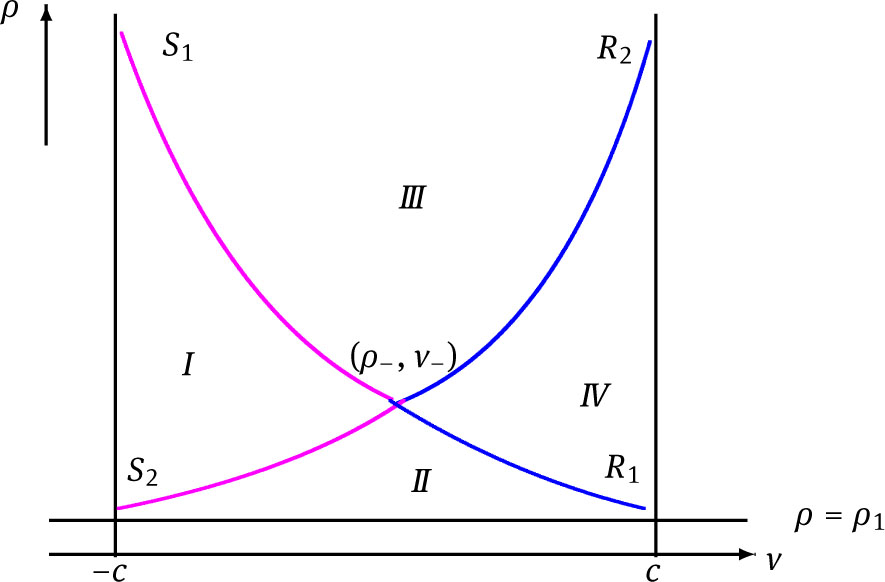
By combining (2.15), (2.16), (2.22) and (2.23), it is clear that the elementary wave curves R₁(ρ_–, v_–), R₂(ρ_–, v_–), S₁(ρ_–, v_–) and S₂(ρ_–, v_–) emanating from the fixed left state (ρ_–, v_–) divide the half-upper (ρ, v) phase plane into four regions I, II, III and IV (see Fig.1). Let (ρ_–, v_–) be fixed, then the solution to the Riemann problem (1.1)-(1.3) is determined uniquely by the above four regions. More precisely, the solution can be expressed as S₁ + S₂ when (ρ₊, v₊) ∈ I, R₁ + S₂ when (ρ₊, v₊) ∈ II, S₁ + R₂ when (ρ₊, v₊) ∈ III or R₁ + R₂ when (ρ₊, v₊) ∈ IV respectively. Here and in what follows, the symbol S₁ + S₂ is adopted to represent a 1-shock wave S₁ followed by a 2-shock wave S₂, etc.

Fig. 1

For the given left state (ρ_–, v_–), the elementary wave curves emanating from the fixed left state (ρ_–, v_–) are shown in the half-upper (ρ, v) phase plane for the Riemann problem (1.1)-(1.3).

References

[1] Anile A., Relativistic Fluids and Magneto-Fluids: with Applications in Astrophysics and Plasma Physics, Cambridge Monographs on Mathematical Physics, Cambridge University Press, Cambridge, 1989.10.1017/CBO9780511564130Search in Google Scholar
[2] Taub A.H., Relativistic Rankine-Hugoniot equations, Phys. Rev., 1948, 74, 328-334.10.1103/PhysRev.74.328Search in Google Scholar
[3] Smoller J., Temple B., Global solutions of the relativistic Euler equations, Commun. Math. Phys., 1993, 156, 67-99.10.1007/BF02096733Search in Google Scholar
[4] Marti J.M., Muller E., The analytical solution of the Riemann problem in relativistic hydrodynamics, J. Fluid Mech., 1994, 258, 317-333.10.1017/S0022112094003344Search in Google Scholar
[5] Chen J., Conservation laws for the relativistic p-system, Commun. Partial Differential Equations, 1995, 20, 1605-1646.10.1080/03605309508821145Search in Google Scholar
[6] Chen G., Li Y., Stability of Remiann solutions with large oscillation for the relativistic Euler equations, J. Differential Equations, 2004, 202, 332-353.10.1016/j.jde.2004.02.009Search in Google Scholar
[7] Li Y., Feng D., Wang Z., Global entropy solutions to the relativistic Euler equations for a class of large initial data, Z. Angew. Math. Phys., 2005, 56, 239-253.10.1007/s00033-005-4118-2Search in Google Scholar
[8] Pourhassan B., Kahya E.O., Extended Chaplygin gas model, Results in Physics, 2014, 4, 101-102.10.1016/j.rinp.2014.05.007Search in Google Scholar
[9] Pourhassan B., Extended Chaplygin gas in Horava-Lifshitz gravity, Physics of the Dark Universe, 2016, 13, 132-138.10.1016/j.dark.2016.06.002Search in Google Scholar
[10] Chaplygin S., On gas jets, Sci. Mem. Moscow Univ. Math. Phys., 1904, 21, 1-121.Search in Google Scholar
[11] Bento M.C., Bertolami O., Sen A.A., Generalized Chaplygin gas, accelerated expansion, and dark-energy-matter unification, Phys. Rev. D, 2002, 66, Article ID 043507.10.1103/PhysRevD.66.043507Search in Google Scholar
[12] Bilic N., Tupper G.B., Viollier R.D., Unification of dark matter and dark energy: the inhomogeneous Chaplygin gas, Physics Letters B, 2012, 535, 17-21.10.1016/S0370-2693(02)01716-1Search in Google Scholar
[13] Debnath U., Banerjee A., Chakraborty S., Role of modified Chaplygin gas in accelerated universe, Classical Quantum Gravity, 2004, 21, 5609-5618.10.1088/0264-9381/21/23/019Search in Google Scholar
[14] Heydarzade Y., Darabi F., Atazadeh K., Einstein static universe on the brane supported by extended Chaplygin gas, Astrophys Space Sci, 2016, 361, Article ID 250.10.1007/s10509-016-2836-7Search in Google Scholar
[15] Kahya E.O., Khurshudyan M., Pourhassan B., Myzakulov R., Pasqua A., Higher order corrections of the extended Chaplygin gas cosmology with varying G and Λ, Eur.Phys.J.C, 2015, 75, Article ID 43.10.1140/epjc/s10052-015-3263-6Search in Google Scholar
[16] Paul B.C., Thakur P., Saha A., Observational constraints on extended Chaplygin gas cosmologies, Pramana J. Phys.,2017, 89, Article ID 29.10.1007/s12043-017-1417-9Search in Google Scholar
[17] Geng Y., Li Y., Non-relativistic global limits of entropy solutions to the extremely relativistic Euler equations, Z.Angew. Math. Phys., 2010, 61, 201-220.10.1007/s00033-009-0031-1Search in Google Scholar
[18] Ding M., Li Y., Non-relativistic limits of rarefaction wave to the 1-D piston problem for the isentropic relativistic Euler equations, J. Math. Phys., 2017, 58, Article ID 081510.10.1063/1.4997873Search in Google Scholar
[19] Sheng W, Zhang T., The Riemann problem for the transportation equations in gas dynamics, Mem.Amer.Math.Soc., 1999, 137, Article ID N654.10.1090/memo/0654Search in Google Scholar
[20] Shen C., Sun M., A distributional product approach to the delta shock wave solution for the one-dimensional zero-pressure gas dynamics system, International Journal of Non-linear Mechanics, 2018, 105, 105-112.10.1016/j.ijnonlinmec.2018.06.008Search in Google Scholar
[21] Li J., Note on the compressible Euler equations with zero temperature, Appl. Math. Lett., 2001, 14, 519-523.10.1016/S0893-9659(00)00187-7Search in Google Scholar
[22] Chen G., Liu H., Formation of Delta-shocks and vacuum states in the vanishing pressure limit of solutions to the isentropic Euler equations, SIAM J. Math.Anal., 2003, 34, 925-938.10.1137/S0036141001399350Search in Google Scholar
[23] Mitrovic D., Nedeljkov M., Delta-shock waves as a limit of shock waves, J. Hyperbolic Differential Equations, 2007, 4, 629-653.10.1142/S021989160700129XSearch in Google Scholar
[24] Chen G., Liu H., Concentration and cavitation in the vanishing pressure limit of solutions to the Euler equations for nonisentropic fluids, Phys. D, 2004, 189, 141-165.10.1016/j.physd.2003.09.039Search in Google Scholar
[25] Shen C., The limits of Riemann solutions to the isentropic magnetogasdynamics, Appl.Math.Lett., 2011, 24, 1124-1129.10.1016/j.aml.2011.01.038Search in Google Scholar
[26] Shen C., Sun M., Formation of delta shocks and vacuum states in the vanishing pressure limit of Riemann solutions to the perturbed Aw-Rascle model, J. Differential Equations, 2010, 249, 3024-3051.10.1016/j.jde.2010.09.004Search in Google Scholar
[27] Sun M., The limits of Riemann solutions to the simplified pressureless Euler system with flux approximation, Math. Methods Appl.Sci., 2018, 41, 4528-4548.10.1002/mma.4912Search in Google Scholar
[28] Wang G., The Remiann problem for one dimensional generalized Chaplygin gas dynamics, J. Math. Anal. Appl., 2013, 403, 434-450.10.1016/j.jmaa.2013.02.026Search in Google Scholar
[29] Shen C., The Riemann problem for the Chaplygin gas equations with a source term, Z. Angew. Math. Mech., 2016, 96, 681-695.10.1002/zamm.201500015Search in Google Scholar
[30] Nedeljkov M., Higher order shadow waves and delta shock blow up in the Chaplygin gas, J. Differential Equations, 2014, 256, 3859-3887.10.1016/j.jde.2014.03.002Search in Google Scholar
[31] Nedeljkov M., Ruzicic S., On the uniqueness of solution to generalized Chaplygin gas, Discrete Contin. Dyn. Syst., 2017, 37, 4439-4460.10.3934/dcds.2017190Search in Google Scholar
[32] Pang Y., Delta shock wave in the compressible Euler equations for a Chaplygin gas, J. Math. Anal. Appl., 2017, 448, 245-261.10.1016/j.jmaa.2016.10.078Search in Google Scholar
[33] Sheng W., Wang G., Yin G., Delta wave and vacuum state for generalized Chaplygin gas dynamics system as pressure vanishes, Nonlinear Anal. RWA, 2015, 22, 115-128.10.1016/j.nonrwa.2014.08.007Search in Google Scholar
[34] Chen J., Sheng W., The Riemann problem and the limit solutions as magnetic field vanishes to magnetogasdynamics for generalized Chaplygin gas, Commun. Pure Appl. Anal., 2018, 17, 127-142.10.3934/cpaa.2018008Search in Google Scholar
[35] Yang H., Wang J., Concentration in vanishing pressure limit of solutions to the modified Chaplygin gas equations, J. Math. Phys., 2016, 57, Article ID 111504.10.1063/1.4967299Search in Google Scholar
[36] Guo L., Li T., Yin G., The vanishing pressure limits of Riemann solutions to the Chaplygin gas equations with a source term, Commun. Pure Appl. Anal., 2017, 16, 295-309.10.3934/cpaa.2017014Search in Google Scholar
[37] Guo L., Li T., Yin G., The limit behavior of the Riemann solutions to the generalized Chaplygin gas equations with a source term, J. Math. Anal. Appl., 2017, 455, 127-140.10.1016/j.jmaa.2017.05.048Search in Google Scholar
[38] Tong M., Shen C., Lin X., The asymptotic limits of Riemann solutions for the isentropic extended Chaplygin gas dynamic system with the vanishing pressure, Boundary Value Problems, 2018, 2018, Article ID 144.10.1186/s13661-018-1064-1Search in Google Scholar
[39] Yin G., Sheng W., Delta shocks and vacuum states in vanishing pressure limits of solutions to the relativistic Euler equations, Chinese Annals of Mathematics, Series B, 2009, 29, 611-622.10.1007/s11401-008-0009-xSearch in Google Scholar
[40] Yin G., Sheng W., Delta shocks and vacuum states in vanishing pressure limits of solutions to the relativistic Euler equations for the polytropic gases, J. Math. Anal. Appl., 2009, 335, 594-605.10.1016/j.jmaa.2009.01.075Search in Google Scholar
[41] Li H., Shao Z., Delta shocks and vacuum states in vanishing pressure limits of solutions to the relativistic Euler equations for generalized Chaplygin gas, Commun. Pure Appl. Anal., 2016, 15, 2373-2400.10.3934/cpaa.2016041Search in Google Scholar
[42] Yin G., Sheng W., Delta wave formation and vacuum state in vanishing pressure limit for system of conservation laws to relativistic fluid dynamics, Z.Angew. Math. Mech., 2015, 95, 49-65.10.1002/zamm.201200148Search in Google Scholar
[43] Yin G., Song K., Vanishing pressure limits of Riemann solutions to the isentropic relativistic Euler system for Chaplygin gas, J. Math. Anal. Appl., 2014, 411, 506-521.10.1016/j.jmaa.2013.09.050Search in Google Scholar
[44] Yang H., Zhang Y., Flux approximation to the isentropic relativistic Euler equations, Nonlinear Anal. TMA, 2016, 133, 200-227.10.1016/j.na.2015.12.002Search in Google Scholar
[45] Sun M., Singular solutions to the Riemann problem for a macroscopic production model, Z.Angew. Math. Mech., 2017, 97, 916-931.10.1002/zamm.201600171Search in Google Scholar
[46] Xu Y., Wang L., Breakdown of classical solutions to Cauchy problem for inhomogeneous quasilinear hyperbolic systems, Indian J. Pure Appl. Math., 2015, 46, 827-851.10.1007/s13226-015-0156-1Search in Google Scholar
[47] Danilov V.G., Shelkovich V.M., Dynamics of propagation and interaction of δ-shock waves in conservation law systems, J. Differential Equations, 2005, 211, 333-381.10.1016/j.jde.2004.12.011Search in Google Scholar
[48] Danilov V.G., Mitrovic D., Delta shock wave formation in the case of triangular hyperbolic system of conservation laws, J.Differential Equations, 2008, 245, 3704-3734.10.1016/j.jde.2008.03.006Search in Google Scholar
[49] Danilov V.G., Nonsmooth nonoscillating exponential-type asymptotics for linear parabolic PDE, SIAM J. Math. Anal., 2017, 49, 3550-3572.10.1137/15M1053311Search in Google Scholar
[50] Kalisch H., Mitrovic D., Singular solutions of a fully nonlinear 2×2 system of conservation laws, Proceedings of the Edinburgh Mathematical Society, 2012, 55, 711-729.10.1017/S0013091512000065Search in Google Scholar
[51] Tartar L., Compensated compactness and applications to partial differential equations, in Res. Notes in Math., Vol.39: Nonlinear Analysis and Mechanics: Heriot-Watt Symposium, Vol. IV, Pitman, Boston, MA, 1979, 136-212.Search in Google Scholar
[52] Murat F., Compacit par compensation, Ann. Scuola Norm. Sup. Pisa Cl. Sci., 1978, 5, 489-507.Search in Google Scholar
[53] Panov E.Yu., Long time asymptotics of periodic generalized entropy solutions of scalar conservation laws, Mathematical Notes, 2016, 100, 113-122.10.1134/S0001434616070105Search in Google Scholar
© 2019 Zhang et al., published by De Gruyter
This work is licensed under the Creative Commons Attribution 4.0 Public License.
Articles in the same Issue
- Regular Articles
- On the Gevrey ultradifferentiability of weak solutions of an abstract evolution equation with a scalar type spectral operator of orders less than one
- Centralizers of automorphisms permuting free generators
- Extreme points and support points of conformal mappings
- Arithmetical properties of double Möbius-Bernoulli numbers
- The product of quasi-ideal refined generalised quasi-adequate transversals
- Characterizations of the Solution Sets of Generalized Convex Fuzzy Optimization Problem
- Augmented, free and tensor generalized digroups
- Time-dependent attractor of wave equations with nonlinear damping and linear memory
- A new smoothing method for solving nonlinear complementarity problems
- Almost periodic solution of a discrete competitive system with delays and feedback controls
- On a problem of Hasse and Ramachandra
- Hopf bifurcation and stability in a Beddington-DeAngelis predator-prey model with stage structure for predator and time delay incorporating prey refuge
- A note on the formulas for the Drazin inverse of the sum of two matrices
- Completeness theorem for probability models with finitely many valued measure
- Periodic solution for ϕ-Laplacian neutral differential equation
- Asymptotic orbital shadowing property for diffeomorphisms
- Modular equations of a continued fraction of order six