On arithmetic–geometric eigenvalues of graphs
-
Bilal A. Rather
 and
Shariefuddin Pirzada
and
Shariefuddin Pirzada

Abstract
In this article, we are interested in characterizing graphs with three distinct arithmetic–geometric eigenvalues. We provide the bounds on the arithmetic–geometric energy of graphs. In addition, we carry out a statistical analysis of arithmetic–geometric energy and boiling point of alkanes. We observe that arithmetic–geometric energy is better correlated with a boiling point than the arithmetic–geometric index.
1 Introduction
A graph
The adjacency matrix
The energy (Gutman, 1978) of
For more about the energy of
The arithmetic–geometric matrix
The
The arithmetic–geometric index (shortly
The
The arithmetic–geometric energy (
For recent work regarding the
In Section 2, we characterize graphs with two distinct
2 AG-eigenvalues of graphs
A natural problem in the spectral theory of graph matrices is the following.
Problem 1
For a connected graph
This problem has been considered for the adjacency matrix, the normalized Laplacian matrix, the distance matrix, etc., for a small value of
It is trivial that
The following well-known result provides a relationship between the number of distinct eigenvalues in a graph and its diameter. It can be found in Brouwer and Haemers (2010).
Theorem 2.1
Let
The proof provided in Brouwer and Haemers (2010) shows that the above result is true for any nonnegative symmetric matrix
Corollary 2.2
If
Another immediate consequence is next stated.
Corollary 2.3
Let
Proof
The
Conversely, if
A set
Next, we have a result that helps us in finding some
Theorem 2.4
Let
if S is a clique of G, then −1 is the AG-eigenvalue of G with multiplicity at least I −1,
if
Proof
We prove point 1 in Theorem 2.4, and then point 2 in Theorem 2.4 can be proved similarly. Suppose that vertices of S form a clique. As vertices of S share the same neighborhood, it follows that
For
Noting that the rows of M are identical, we see that:
Similarly, we can easily see that
Next, if S forms an independent set, then with the same set of vectors, we can see that 0 is the AG-eigenvalues of G with multiplicity I − 1.
Theorem 2.4 helps us to obtain the AG-eigenvalues of some well-known families of graphs. In the following result, we mention some of these families.□
Proposition 2.5
Let G be a connected graph of order n . Then, the following statements hold:
The AG-spectrum of
The AG -spectrum of the complete split graph
where
3. The
4. The
AG
-spectrum of
Proof
As
which are
As
It follows from (ii), with
As above, we can verify that
The other three
The characteristic polynomial of the above matrix is:
For
From the above calculations and by intermediate value theorem, it follows that the matrix in Eq. 1 has three distinct eigenvalues.
From point 1 in Proposition 2.5, we can state the following observation.□
Remark 2.6
All complete bipartite graphs on the same order
We observe that the
If
This implies that
The next result (Liu and Shiu, 2015) states the distinct eigenvalues of irreducible non-negative symmetric real matrix.
Theorem 2.7
Let
Further,
Corollary 2.8
Let
Further,
Proof
Since
Corollary 2.2 plays the fundamental role in characterizing graphs with distinct eigenvalues and helps in solving Problem 1 for
Corollary 2.9
Let
Proof
By Corollary 2.8,
Now, comparing the diagonal entries and the off-diagonal entries of the above equation, we get the desired result.□
Suppose we have a matrix
For graphs with diameters greater or equal to three, Corollary 2.2 confirms that
Proposition 2.10
Let
if
if
if
Proof
Assume that
Conversely, if
Next,
If
and it proves that Eq. 2 has three distinct
It can be easily verified that the above expression has a positive determinant, which gives us that
For the general case of
For
and it is easy to see that
Consider
for
and it is clear that it has two distinct eigenvalues. Thus the biregular complete multipartite has more than three
Lastly, if
and so the result follows in this case.□
Remark 2.11
There exists graphs, other than those characterized in Proposition 2.10 with exactly three distinct
Further, we see that their complements also have three distinct
Above remark give an insight that there can be more graphs with exactly three distinct
Problem 2
Characterize all graphs having exactly three distinct AG-eigenvalues.

Graphs with three distinct
3
AG
-energy of graphs
Let
where
Our first result gives an upper bound on the
Theorem 3.1
Let
Proof
Using the fact that
Now, using the above information, inequality (Eq. 6) is equivalent to:
Recall that
Lastly, using all the above information, we have:
thus proves the result.□
The following result is the immediate consequence of Theorems
Corollary 3.2
Let
equality holding if and only if
Proof
From the proof of Theorem
with equality if and only if
By comparing these two expressions, we obtain:
which implies that:
Therefore, by definition of
Since, for graphs with exactly one positive
Remark 3.3
From the proof of Theorem 4.1 from Guo and Gao (2020), we have:
with equality if and only if
which gives us
Theorem 3.4
Let
Proof
As
Now, consider the function:
It is easy to verify that
Recalling that
Combining the above inequality with Eq. 8, we obtain the required inequality (point 1 in Theorem 3.4).
For the second part, proceeding as above and using the fact that
4 Statistical analysis
We carried out a statistical study to compare the correlation of the boiling point of chemical compounds with the arithmetic–geometric index
Our data, given in Table 1, consist of the boiling point
Boiling point,
| Name | Bp | AG |
|
Name | Bp | AG |
|
Name | Bp | AG |
|
|---|---|---|---|---|---|---|---|---|---|---|---|
| n1 | −161.5 | 0 | 0 | 1tbc3 | 80.5 | 7.8016 | 8.67379 | b2mc3 | 124 | 8.27722 | 10.3517 |
| n2 | −88.6 | 1 | 2 | 11ec3 | 88.6 | 7.36396 | 9.27722 | 1nepec3 | 106 | 8.87252 | 9.74915 |
| n3 | −42.1 | 2.12132 | 3 | 1e23mc3 | 91 | 7.39068 | 8.99593 | 5msbc3 | 115.5 | 8.50534 | 10.3518 |
| c3 | −32.8 | 3 | 4 | 1m1ipce | 81.5 | 7.69108 | 9.01389 | 1e2pc3 | 108 | 8.2038 | 10.3045 |
| n4 | −0.5 | 3.12132 | 4.69042 | 11m23c3 | 79.1 | 7.67292 | 8.90465 | ib2mc3 | 110 | 8.54658 | 9.86825 |
| 2mn3 | −11.7 | 3.4641 | 4 | 12m1ec3 | 85.2 | 7.61766 | 9.05318 | 11m2pc3 | 105.9 | 8.67292 | 9.91127 |
| 1mc3 | −0.7 | 4.19594 | 5.23802 | 1123mc3 | 78 | 7.83013 | 9.18966 | 1m12epc3 | 108.9 | 8.54425 | 10.5422 |
| c4 | 12.6 | 4 | 4 | 1122mc3 | 76 | 8.12132 | 8.41765 | 11m2ipc3 | 94.4 | 8.90104 | 9.9405 |
| bc110b | 8 | 5.08248 | 5.20317 | 1pc4 | 100.7 | 7.12252 | 8.28829 | 112m2ec3 | 104.5 | 8.99262 | 10.0879 |
| n5 | 36 | 4.12132 | 5.65685 | 1ipc4 | 92.7 | 7.35064 | 7.72793 | 11223mc3 | 100.5 | 9.17543 | 10.2962 |
| 2mn4 | 27.8 | 4.39068 | 5.76105 | 1e3mc4 | 89.5 | 7.31846 | 8.52598 | 1ibc4 | 120.1 | 8.39188 | 9.33738 |
| 22mn3 | 9.5 | 5 | 5 | 1e2mc4 | 94 | 7.27722 | 8.63449 | p3mc4 | 117.4 | 8.31846 | 9.52741 |
| 1ec3 | 35.9 | 5.12252 | 6.60537 | 1ec5 | 103.5 | 7.12252 | 9.09223 | 1sbc4 | 123 | 8.27722 | 9.41768 |
| 12mc3 | 32.6 | 5.35064 | 6.34632 | 13mc5 | 91.3 | 7.39188 | 8.84221 | 12ec4 | 119 | 8.2038 | 9.51732 |
| 11mc2 | 20.6 | 5.62132 | 6.31872 | 12mc5 | 95.6 | 7.35064 | 8.94888 | 1234mc4 | 114.5 | 8.6188 | 10.7289 |
| 1mc4 | 36.3 | 5.19594 | 5.89327 | 11mc5 | 87.9 | 7.62132 | 8.81715 | 1133mc4 | 86 | 9.24264 | 9.05821 |
| c5 | 49.3 | 5 | 6.47214 | 1mc6 | 101 | 7.19594 | 8.96625 | 1pc5 | 131 | 8.12252 | 10.2194 |
| bc111p | 36 | 6.12372 | 5 | c7 | 118.4 | 7 | 8.98792 | 1ipc5 | 126.4 | 8.35064 | 10.134 |
| bc210p | 46 | 6.08248 | 6.44846 | dcprm | 102 | 8.12372 | 9.76269 | 1e3mc5 | 121 | 8.31846 | 10.3594 |
| s22p | 39 | 6.24264 | 7.3589 | bc221h | 105.5 | 8.12372 | 9.76269 | 1e2mc5 | 124.7 | 8.27722 | 10.3557 |
| mbc110b | 33.5 | 6.42292 | 6.56159 | bc311h | 110 | 8.12372 | 9.2473 | 124mc5 | 115 | 8.54658 | 9.94485 |
| n6 | 68.7 | 5.12132 | 7.20036 | bc320h | 110.5 | 8.08248 | 9.01277 | 1e1mc5 | 121.5 | 8.49264 | 10.4653 |
| 2mn5 | 60.3 | 5.39068 | 6.65235 | bc410h | 116 | 8.08248 | 9.75124 | 123mc5 | 117 | 8.50534 | 10.6077 |
| 3mn5 | 63.3 | 5.31726 | 7.40948 | s33h | 96.5 | 8.24264 | 7.92745 | 113mc5 | 104.5 | 8.81726 | 9.8801 |
| 23mn4 | 58 | 5.6188 | 6.8313 | s24h | 98.5 | 8.24264 | 9.33053 | 112mc5 | 114 | 8.74634 | 10.0141 |
| 22mn4 | 49.7 | 5.87132 | 6.79126 | 2mbc310hx | 100 | 8.23718 | 9.72558 | 1ec6 | 131.8 | 8.12252 | 10.6021 |
| 1pc3 | 69 | 6.12252 | 7.71721 | 6mbc310hx | 103 | 8.19594 | 9.68638 | 14mc6 | 121.8 | 8.39188 | 10.476 |
| 1ipc3 | 58.3 | 6.35064 | 7.65407 | mbc210hx | 81.5 | 8.49384 | 9.08634 | 13mc6 | 122.3 | 8.39188 | 9.9193 |
| 1e2mc3 | 63 | 6.27722 | 7.83428 | mbc310hx | 92 | 8.42292 | 9.55002 | 12mc6 | 126.6 | 8.35064 | 10.4828 |
| 1e1mc3 | 57 | 6.49262 | 7.9621 | 13mbc111p | 71.5 | 8.86396 | 8.26628 | 11mc6 | 119.5 | 8.62132 | 9.95609 |
| 123mc3 | 63 | 6.4641 | 8.08827 | 14mbc210p | 74 | 8.74264 | 9.45753 | 1mc7 | 134 | 8.19594 | 10.2688 |
| 112mc3 | 52.6 | 6.74634 | 7.38891 | 11ms22p | 78 | 8.74262 | 9.46973 | c8 | 149 | 8 | 9.65685 |
| 1ec4 | 70.7 | 6.12252 | 6.75811 | 122mbcb | 84 | 8.85201 | 9.5329 | bcprm | 129 | 9.12372 | 10.9685 |
| 13mc4 | 59 | 6.39188 | 6.99982 | tc410024h | 105 | 9.12372 | 10.349 | bc330o | 137 | 9.08248 | 10.5425 |
| 12mc4 | 62 | 6.35064 | 7.78216 | tc311024h | 107 | 9.12372 | 9.6418 | bcb | 136 | 9.08248 | 9.31797 |
| 11mc4 | 53.6 | 6.62132 | 7.03562 | tc221026h | 106 | 9.12372 | 10.3583 | bc4200 | 133 | 9.08248 | 10.4596 |
| 1mc5 | 51.8 | 6.19594 | 7.74106 | tc410027h | 110 | 9.04124 | 10.3032 | bc510o | 141 | 9.08248 | 10.5556 |
| c6 | 80.7 | 6 | 8 | tc410013h | 107.5 | 9.22453 | 10.4529 | 2mbc221h | 125 | 9.27842 | 10.8884 |
| bc211hx | 71 | 7.12372 | 7.6929 | tec320h | 108.5 | 10.0412 | 10.2998 | S34o | 128 | 9.24264 | 10.2471 |
| bcpr | 76 | 7.08248 | 8.39864 | tec410h | 104 | 10.0412 | 10.7088 | 7mbc320h | 128 | 9.23718 | 11.1892 |
| bc220hx | 83 | 7.08248 | 7.7735 | n8 | 125.7 | 7.12132 | 9.7278 | 2mbc320h | 130.5 | 9.23718 | 10.0441 |
| bc310hx | 81 | 7.08248 | 8.4923 | 2mn7 | 117.6 | 7.39068 | 9.27007 | s25o | 125 | 9.24264 | 11.0911 |
| s23hx | 69.5 | 7.24264 | 7.75831 | 3mn7 | 118.9 | 7.31726 | 9.9114 | 1mbc221h | 117 | 9.49384 | 10.9527 |
| mbc210p | 60.5 | 7.42292 | 8.20672 | 4mn7 | 117.7 | 7.31726 | 9.26915 | 7mbc410h | 138 | 9.19594 | 11.1487 |
| 13mbcb | 55 | 7.74264 | 7.71752 | 25mn6 | 109.1 | 7.66004 | 9.31019 | 1mbc410h | 125 | 9.42292 | 10.94 |
| n7 | 98.5 | 6.12132 | 8.25402 | 3en6 | 118.5 | 7.24384 | 9.83204 | 33mbc310hx | 115 | 9.7038 | 10.4437 |
| 2mn6 | 90 | 6.39068 | 8.25215 | 24mn6 | 109.4 | 7.58662 | 9.3399 | 14mbc211hx | 91 | 9.86396 | 10.2359 |
| 3mn6 | 92 | 6.31726 | 8.35197 | 23mn6 | 115.6 | 7.54538 | 9.41305 | 66mbc310hx | 126.1 | 9.56197 | 10.7436 |
| 3en5 | 93.5 | 6.24384 | 8.36575 | 34mn6 | 117.7 | 7.47196 | 10.106 | 2244mbcb | 104 | 10.0415 | 10.4453 |
| 24mn5 | 80.5 | 6.66004 | 7.62489 | 22mn6 | 106.8 | 7.87132 | 9.27384 | 1223mbcb | 105 | 10.1213 | 10.7638 |
| 23mn5 | 89.8 | 6.54538 | 8.46557 | 3e2mn5 | 115.6 | 7.47196 | 9.35947 | tc510035o | 142 | 10.165 | 11.3133 |
| 22mn5 | 79.2 | 6.87132 | 7.65211 | 234mn5 | 113.5 | 7.7735 | 9.51778 | tc510024o | 149 | 10.1237 | 11.4555 |
| 33mn5 | 86.1 | 6.74264 | 8.52444 | 33mn6 | 112 | 7.74264 | 9.40615 | tc3210o | 136 | 10.1237 | 11.6894 |
| 223mn4 | 80.9 | 7.06976 | 7.8603 | 224mn5 | 99.2 | 8.14068 | 8.61401 | tc3300o | 125 | 10.0825 | 11.1747 |
| 1bc3 | 98 | 7.12252 | 9.11395 | 3e3mn5 | 118.2 | 7.61396 | 10.1466 | 3mtc2210h | 120.5 | 10.2372 | 11.636 |
| 1sbc3 | 90.3 | 7.27722 | 9.29729 | 223mn5 | 109.8 | 7.99634 | 9.48833 | ds2121o | 103 | 10.4853 | 11.1026 |
| 1m2pc3 | 93 | 7.27722 | 8.85944 | 233mn5 | 114.8 | 7.94108 | 9.58514 | 1mtc2210h | 111 | 10.4345 | 11.5024 |
| 12ec3 | 90 | 7.2038 | 9.17525 | 2233mn4 | 106.5 | 8.5 | 8.88819 | ds2022o | 115 | 10.364 | 11.4681 |
| 1m1pc3 | 84.9 | 7.49264 | 8.88115 | 1pec3 | 128 | 8.12252 | 10.2807 | tec330o | 137.5 | 11.0825 | 12.2547 |
| 1m2ipc3 | 81.1 | 7.50534 | 8.87111 | 1spec3 | 117.4 | 8.27722 | 10.2413 |
The most important observation is that
Figure 2 illustrates the linear regression between the boiling point and

Linear regression
Figure 3 shows the linear regression between the boiling point and

Linear regression
The linear regression shows that the correlation of the boiling point is better with
Figure 4 illustrates the logarithmic regression between the boiling point and

Logarithmic regression
Figure 5 shows the logarithmic regression between the boiling point and

Logarithmic regression
The logarithmic regression shows that the correlation of the boiling point is better with
Figure 6 illustrates the quadratic regression between the boiling point and

Quadratic regression
Figure 7 shows the quadratic regression between the boiling point and
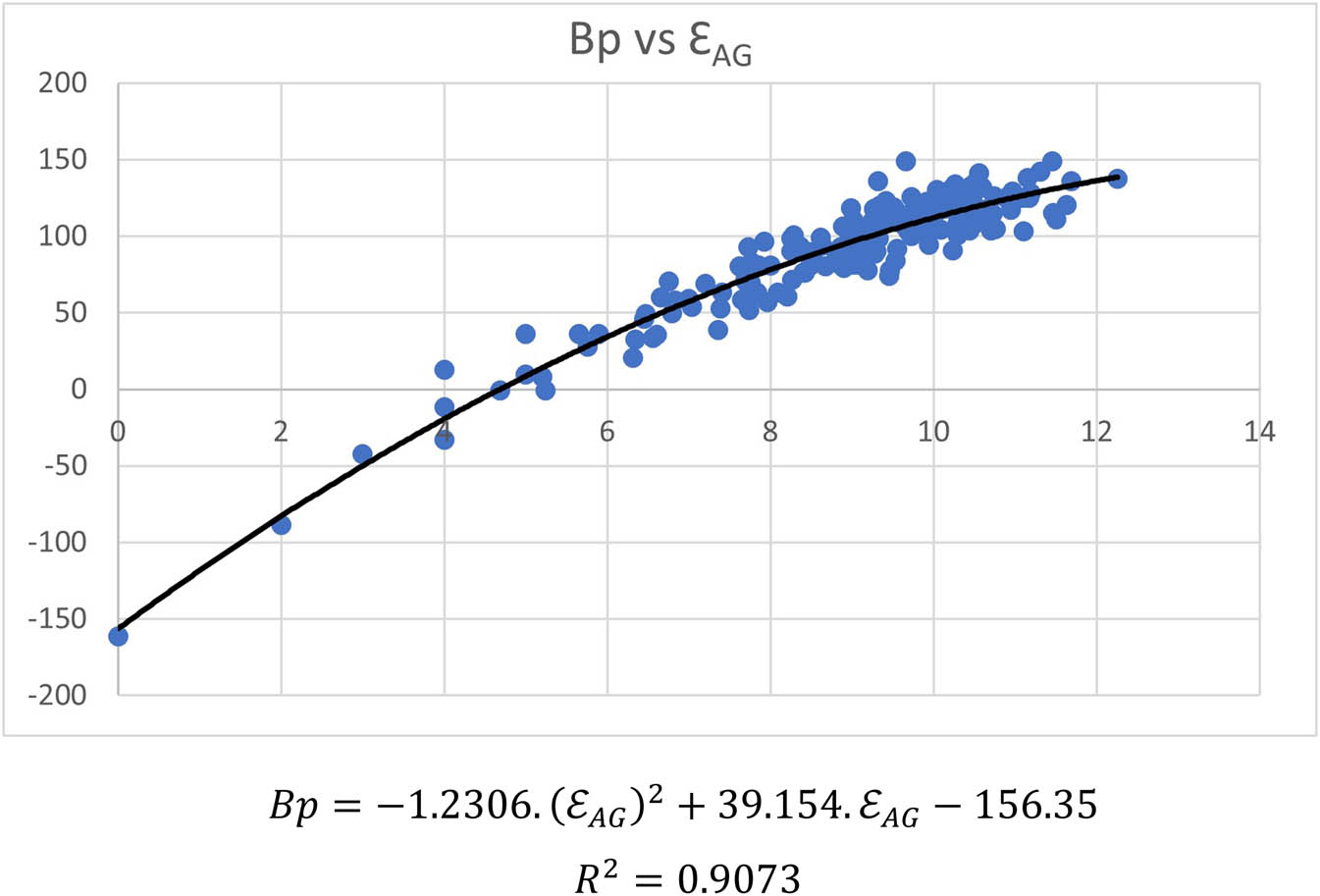
Quadratic regression
The quadratic regression shows that the correlation of the boiling point is better with
The study shows that in each regression model, the boiling point is better correlated with the arithmetic–geometric energy than with the arithmetic–geometric index. Comparing the models, the logarithmic regression gives a better correlation. Overall, the best correlation with boiling point is obtained with the arithmetic–geometric energy using the logarithmic regression.
5 Conclusions
The result in this article characterizes certain classes of graphs with three distinct
Acknowledgment
We are highly thankful to the Editor and the referees for their valuable comments and suggestions. These suggestions have considerably improved the presentation of the article.
-
Funding information: United Arab Emirates University (grant no. G00003461).
-
Author contributions: Bilal A. Rather: writing – original draft, writing – review and editing, formal analysis; Mustapha Aouchiche: writing – original draft, methodology, formal analysis, visualization, and project administration; Muhammad Imran: writing – original draft, formal analysis, and visualization; Shariefuddin Pirzada: formal analysis, methodology, and writing – editing.
-
Conflict of interest: The corresponding author (Muhammad Imran) is a Guest Editor of the Main Group Metal Chemistry's Special Issue “Theoretical and computational aspects of graph-theoretic methods in modern-day chemistry” in which this article is published.
-
Data availability statement: There are no data associated with this article
References
Alazemi A., Andelić M., Koledin T., Stanić Z., Distance-regular graphs with small number of distinct distance eigenvalues, Linear Algebra Appl., 2017, 531, 83–97.10.1016/j.laa.2017.05.033Search in Google Scholar
Aouchiche M., Ganesan V., Adjusting geometric-arithmetic index to estimate boiling point. Match Commun. Math. Comput. Chem., 2020, 84, 483–497.Search in Google Scholar
Aouchiche M., Hansen P., The normalized revised Szeged index. Match Commun. Math. Comput. Chem., 2012, 67, 369–381.Search in Google Scholar
Brouwer A.E., Haemers W.H., Spectra of graphs, Springer, New York, 2010.Search in Google Scholar
Caporossi G., Variable neighborhood search for extremal vertices: The AutoGraphiX-III system. Comput. Oper. Res., 2017, 78 431–438.10.1016/j.cor.2015.12.009Search in Google Scholar
Chen X., On ABC eigenvalues and ABC energy. Linear Algebra Appl. 2018, 544, 141–157.10.1016/j.laa.2018.01.011Search in Google Scholar
Cvetković D.M., Rowlison P., Simić S., An introduction to theory of graph spectra. London mathematics society student text, 75, Cambridge University Press, UK, 2010.10.1017/CBO9780511801518Search in Google Scholar
Estrada E., Atom-bond connectivity and the energetic of branched alkanes, Chem. Phys. Lett., 2008, 463(4–6), 422–425.10.1016/j.cplett.2008.08.074Search in Google Scholar
Guo X., Gao Y., Arithmetic-geometric spectral radius and energy of graphs. Match Commun. Math. Comput. Chem., 2020, 83, 651–660.Search in Google Scholar
Gutman I., The Energy of a graph. Ber. Math. Statist. Sekt. Forschungszenturm Graz., 1978, 103, 1–22.10.1002/9783527627981.ch7Search in Google Scholar
Hosamani S.M., Kulkarni B.B., Boli R.G., Gadag V.M., QSPR analysis of certain graph theoretical matrices and their corresponding energy. Appl. Math. Nonlinear Sci., 2017, 2, 131–150.10.21042/AMNS.2017.1.00011Search in Google Scholar
Huang X., Huang Q., On graphs with three of four distinct normalized Laplacian eigenvalue. Algebra Colloquium, 2019, 26(1), 65–82.10.1142/S1005386719000075Search in Google Scholar
Huang X., Huang Q., Lu L. Graphs with at most three distance eigenvalue different from −1 and −2. Graphs Combinatorics, 2018, 34, 395–414.10.1007/s00373-018-1880-1Search in Google Scholar
Jahanbani A., Lower bounds for the energy of graphs. AKCE Int. J. Graphs Combinatorics, 2018, 15(1), 88–96.10.1016/j.akcej.2017.10.007Search in Google Scholar
Li X., Shi Y., Gutman I., Graph energy, Springer, New York, 2010.Search in Google Scholar
Liu R., Shiu W.C., General Randić matrix and general Randić incidence matrix. Discrete Appl. Math., 2015, 186, 168–175.10.1016/j.dam.2015.01.029Search in Google Scholar
Pirzada S., Rather B.A., Aouchiche M., On eigenvalues and energy of geometric–arithmetic matrix of graphs. Medit. J. Math., 2022, 19, 115. 10.1007/s00009-022-02035-0.Search in Google Scholar
Qi L., Miao L., Zhao W., Lu L. Characterization of graphs with an eigenvalue of large multiplicity. Adv. Math. Physics, 2020, 2020. 10.1155/202/3054672. Search in Google Scholar
Rather B.A., Aouchiche M., Pirzada S., On the spread of the geometric-arithmetic matrix of graphs, AKCE Int. J. Graphs Comb., 2022, 19(2), 146–153. 10.1080/09728600.2022.2088315. Search in Google Scholar
Rather B.A., Imran M., Sharp bounds on the sombor energy of graphs. Match Commun. Math. Comput. Chem., 2022, 88(3), 605–624.10.46793/match.88-3.605RSearch in Google Scholar
Raza Z., Bhatti A.A., Ali A., More on comparison between first geometric–arithmetic index and atom–bond connectivity index. Miskolc Math. Notes, 2016, 17, 561–570.10.18514/MMN.2016.1265Search in Google Scholar
Rowlinson P., More on graphs with just three distinct eigenvalues. Appl. Anal. Discrete Math., 2017, 11, 74–80.10.2298/AADM161111033RSearch in Google Scholar
Rodríguez J.M., Sánchez J.L., Sigarreta J.M., Tourís E., Bounds on the arithmetic-geometric index. Symmetry, 2021, 13(4), 689.10.3390/sym13040689Search in Google Scholar
Rodriguez J.M., Sigarreta J.M., Spectral study of the geometric-arithmetic index. Match Commun. Math. Comput. Chem., 2015, 74, 121–135.Search in Google Scholar
Rücker G., Rücker C., On topological indices, boiling points and cycloalkanes. J. Chem. Inf. Comput. Sci., 1999, 39, 788–802.10.1021/ci9900175Search in Google Scholar
Shegehall V.S., Kanabur R., Arithmetic-geometric indices of path graphs. J. Math. Comput. Sci.,2015, 16, 19–24.Search in Google Scholar
Sun S., Das K.C., On the multiplicities of normalized Laplacian eigenvalues of graphs. Linera Algebra Appl., 2021, 609, 365–385.10.1016/j.laa.2020.09.022Search in Google Scholar
Tian F., Wang Y., Full characterization of graphs having certian normalized Laplacian eigenvalues of multiplicity n − 3. Linear Algebra Appl., 2021, 630, 69–83.10.1016/j.laa.2021.07.024Search in Google Scholar
Vujošević S., Popivoda G., Vukiećević Z.K., Furtula B., Skrekovski R., Arithmetic-geometric index and its relation with arithmetic-geometrix index. Appl. Math. Comput., 2021, 391, 125706.10.1016/j.amc.2020.125706Search in Google Scholar
Wang Y., Gao Y., Nordhaus-Gaddum-type relations for the arithmetic-geometric spectral radius and energy. Math. Problems Eng., 2020, 2020, 5898735.10.1155/2020/5898735Search in Google Scholar
Wang Y., Gao Y., Bounds for the energy of graphs. Math., 2021, 9, 1687.10.3390/math9141687Search in Google Scholar
Zheng L., Tian G.X., Cui S.Y., On spectral radius and energy of arithmetic-geometric matrix of graphs. Match Commun. Math. Comput. Chem., 2020, 83, 635–650.Search in Google Scholar
Zheng L., Tian G.X., Cui S.Y., Arithmetic-geometric energy of specific graphs. Discrete Math. Algorithms Appl., 2021, 215005, 15.10.1142/S1793830921500051Search in Google Scholar
Zheng R., Jin X., Arithmetic-geometric spectral radius of trees and unicyclic graphs. 2021, Arxiv:2015.03884.Search in Google Scholar
© 2022 Bilal A. Rather et al., published by De Gruyter
This work is licensed under the Creative Commons Attribution 4.0 International License.
Articles in the same Issue
- Embedded three spinel ferrite nanoparticles in PES-based nano filtration membranes with enhanced separation properties
- Research Articles
- Syntheses and crystal structures of ethyltin complexes with ferrocenecarboxylic acid
- Ultra-fast and effective ultrasonic synthesis of potassium borate: Santite
- Synthesis and structural characterization of new ladder-like organostannoxanes derived from carboxylic acid derivatives: [C5H4N(p-CO2)]2[Bu2Sn]4(μ3-O)2(μ2-OH)2, [Ph2CHCO2]4[Bu2Sn]4(μ3-O)2, and [(p-NH2)-C6H4-CO2]2[Bu2Sn]4(μ3-O)2(μ2-OH)2
- HPA-ZSM-5 nanocomposite as high-performance catalyst for the synthesis of indenopyrazolones
- Conjugation of tetracycline and penicillin with Sb(v) and Ag(i) against breast cancer cells
- Simple preparation and investigation of magnetic nanocomposites: Electrodeposition of polymeric aniline-barium ferrite and aniline-strontium ferrite thin films
- Effect of substrate temperature on structural, optical, and photoelectrochemical properties of Tl2S thin films fabricated using AACVD technique
- Core–shell structured magnetic MCM-41-type mesoporous silica-supported Cu/Fe: A novel recyclable nanocatalyst for Ullmann-type homocoupling reactions
- Synthesis and structural characterization of a novel lead coordination polymer: [Pb(L)(1,3-bdc)]·2H2O
- Comparative toxic effect of bulk zinc oxide (ZnO) and ZnO nanoparticles on human red blood cells
- In silico ADMET, molecular docking study, and nano Sb2O3-catalyzed microwave-mediated synthesis of new α-aminophosphonates as potential anti-diabetic agents
- Synthesis, structure, and cytotoxicity of some triorganotin(iv) complexes of 3-aminobenzoic acid-based Schiff bases
- Rapid Communications
- Synthesis and crystal structure of one new cadmium coordination polymer constructed by phenanthroline derivate and 1,4-naphthalenedicarboxylic acid
- A new cadmium(ii) coordination polymer with 1,4-cyclohexanedicarboxylate acid and phenanthroline derivate: Synthesis and crystal structure
- Synthesis and structural characterization of a novel lead dinuclear complex: [Pb(L)(I)(sba)0.5]2
- Special Issue: Theoretical and computational aspects of graph-theoretic methods in modern-day chemistry (Guest Editors: Muhammad Imran and Muhammad Javaid)
- Computation of edge- and vertex-degree-based topological indices for tetrahedral sheets of clay minerals
- Structures devised by the generalizations of two graph operations and their topological descriptors
- On topological indices of zinc-based metal organic frameworks
- On computation of the reduced reverse degree and neighbourhood degree sum-based topological indices for metal-organic frameworks
- An estimation of HOMO–LUMO gap for a class of molecular graphs
- On k-regular edge connectivity of chemical graphs
- On arithmetic–geometric eigenvalues of graphs
- Mostar index of graphs associated to groups
- On topological polynomials and indices for metal-organic and cuboctahedral bimetallic networks
- Finite vertex-based resolvability of supramolecular chain in dialkyltin
- Expressions for Mostar and weighted Mostar invariants in a chemical structure