Morse index of circular solutions for repulsive central force problems on surfaces
-
Ran Yang


Abstract
The classical theory of repulsive central force problem on the standard (flat) Euclidean plane can be generalized to surfaces by reformulating the basic underlying physical principles by means of differential geometry. The aim of the present paper is to compute the Morse index of the circular periodic orbits in the case of repulsive power-law potentials of the Riemannian distance on revolution’s surfaces.
1 Description of the problem and main results
Central-force dynamics and orbital motion are fundamental topics in advanced mechanics. In particular, Newtonian mechanics on non-flat spaces can be naturally formulated within the framework of Riemannian geometry. A mechanical system is described by a triple (M, g, V), where M is a smooth manifold representing the configuration space, g is a Riemannian metric that determines the kinetic energy, and V is the potential function.
In Physics and Classical Mechanics, many interactions are modeled by using potentials depending on the distance alone, such as when one studies systems of many particles interacting with each other or when one considers a single particle that interacts with a source. Thus, it seems natural to investigate systems on manifolds M whose potential is a function of the distance from a point.
For attractive central force problem, the Keplerian problem is a classical model. In the last decades, several authors provided a generalization of the gravitational Keplerian potential in the constant curvature case, starting with the well-known manuscript of Harin & Kozlov [1]. Some generalizations can be found in refs. [2], [3], [4] and references therein. Inspired by the approach in ref. [5], in ref. [6] we compute the Morse index of the circular orbits under some attractive power-law potentials of the Riemannian distance on revolution’s surfaces by using the normal form provided in ref. [7].
But some classical repulsive central force problems are excluded, for example, the dynamics of electrons with the same charge. Therefore, in the rest of the paper, we aim to compute the Morse index of the circular periodic orbits in the case of repulsive power-law potentials of the Riemannian distance on revolution’s surfaces which are conformal to the flat one, namely, the sphere and hyperbolic plane. The computation of the Morse index can be reduced to the calculation of the Maslov index associated with the periodic orbit of the corresponding linear Hamiltonian system. For detailed accounts of the Maslov index and its applications to stability problem, we refer the reader to refs. [8], [9], [10], [11], [12], [13], [14], [15], [16], [17], [18], [19], [20], [21], among others.
In polar coordinates ξ, θ and up to rescaling time and normalizing the radial variable, we end up considering the following Lagrangian function
Here p denotes the conformal factor and q the potential. For the sphere and the hyperbolic plane with constant curvature metrics the conformal factors potentials are
(Sphere case)
(1.1)(Hyperbolic plane case)
(1.2)
where x = (ξ, ϑ), T > 0 denotes the prime period of the orbit and A is defined on the Hilbert space of the H 1 loops (of period T) in the punctured plane. We let x be a T-periodic circular orbit, i.e. a solution of the form x(t) = (ξ 0, θ 0 + tω) for t ∈ [0, T/ω]. Denoting by m −(x) the Morse index of the critical point x, our results read as follows.
Theorem 1.
(Sphere Case). Let p and q be as in (1.1), and let x denote a circular solution. Then the Morse index of x is given by
Here,
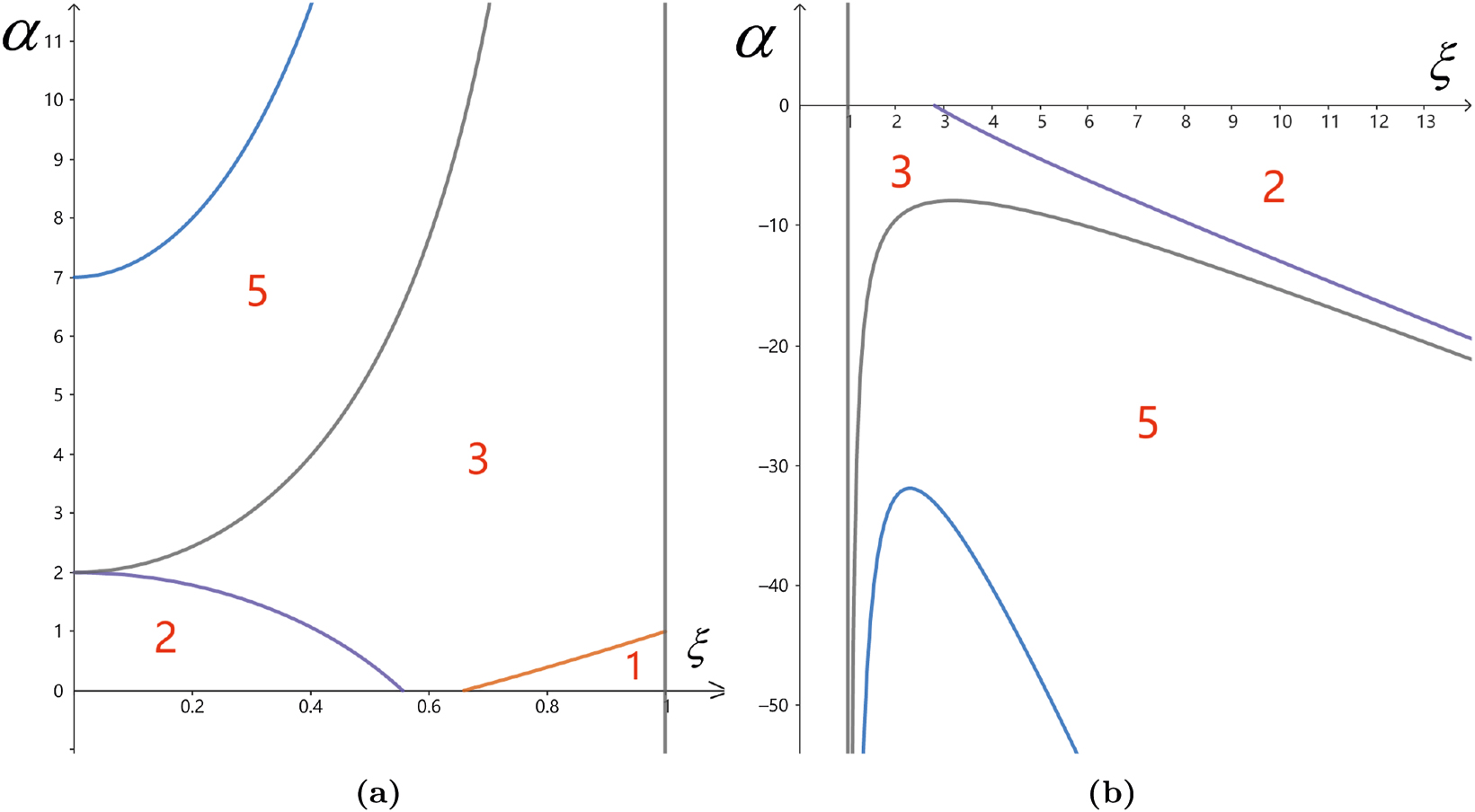
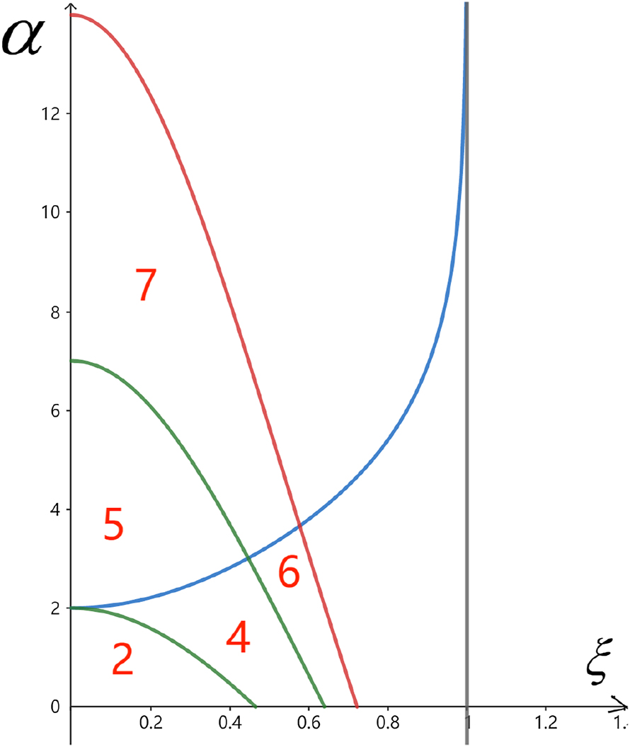
(Sphere case) The subregions of Ω1, Ω2 corresponding to the jumps of the Morse index. (a) (Sphere case α positive) In this figure are displayed the subregions of the
Theorem 2.
(Hyperbolic plane Case). Let p and q be as in (1.2), and let x denote a circular solution. Then the Morse index of x is given by
where
For Euclidean case we have the following result.
(Hyperbolic plane case) In the figure we represent the subregions of the Ω3 corresponding to the jumps of the Morse index.
Theorem 3.
Let p(ξ) = 1, q(ξ) = −ξ α and let x be a circular solution. Then the Morse index of x is given by
2 Central force problem on constant curvature surfaces
We start by considering the configuration space
In terms of the curvature κ, the conformal factor can be written at once as
We now take the origin as the center of the central force and we consider the simple mechanical system (M, g, V) where
Given
and we consider the Lagrangian
By introducing the change of variables ξ ≔ r/R, the Lagrangian function can be rewritten as follows:
Now, computing
and denoting by ⋅ the τ derivative as well, we get that
and C
α
≔ mR
α
2
α
(resp. C ≔ mR
α
) in the case of
2.1 Euler–Lagrange equation and Sturm-Liouville problem
We let
Notation 2.1.
In shorthand notation, with abuse of notation, we use p(ξ) for denoting either p +(ξ) or p −(ξ) and q(ξ) for denoting either q +(ξ) or q −(ξ). Furthermore, we denote by p′ (resp. q′) the ξ derivative of p (resp. q).
Now we can consider the Lagrangian L
α
instead of
and by a direct calculation we get that the associated Euler–Lagrangian equation is
A special class of solutions of the Euler–Lagrange equation is provided by the circular solutions pointwise defined by
Notation 2.2.
We set
So, the period T is given by
By linearizing along x we get the Sturm-Liouville equation given by
where
We set
We observe that
In conclusion, we get
where
Notation 2.3.
We let
Bearing this notation in mind the linear autonomous Hamiltonian system z′(t) = JBz(t) reads as
where
Then we introduce the following formula to compute the Morse index.
Lemma 2.4.
Let
where
Proof.
It is referred to [6], Theorem 1]. □
3 Computations of Morse index for circular orbits
This section is devoted to compute the Morse index of the circular orbits on the sphere, pseudo-sphere and Euclidean plane. We start by recalling that, in this case, the Lagrangian of the problem is given by
3.1 Circular orbits on the sphere
In this case
In order for the (RHS) of
By a direct computation, we get
In order to determine the Morse index, we have to discuss the sign of d according to α and ξ 0.
3.1.1 First case: α positive
Since in this case ξ 0 ∈ (0, 1), then we get that the sign of d is minus the sign of
We let
and it is easy to check that f 1(ξ) > 0 for all (ξ, α) ∈ Ω1 and consequently there always holds d < 0 in Ω1.
Next we need to determine the sign of b 2 + cd. Taking into account Equation (3.2) and after some algebraic manipulations, we have
We observe that, since F(ξ
0) is strictly positive and
According to the sign of f 2(ξ) we can split Ω1 into the following three subregions
By this discussion, we finally get that
In this case for computing the Morse index, we need to calculate the integer k defined by
and using Equation (3.2), we get
Indeed, we can check that for every
For example, by a direct computation, we infer that
So, denoting these regions as follows
we finally get that for any
Similarly, direct computations show that
and so on. Figure 3 are displayed all indices in these involved regions.
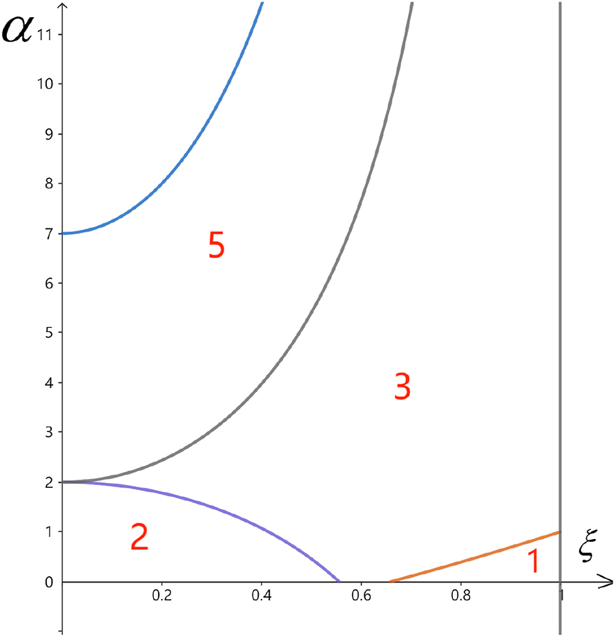
(Sphere case α positive) The subregions of the
By invoking Lemma 2.4 we finally get
3.1.2 Second case: α negative
In this case, by taking into account the restrictions provided at Equation (3.1), we have ξ
0 ∈ (1, +∞) and consequently
We let
and we start observing that the sign of f 1(ξ) defined in (3.3) for (ξ, α) ∈ Ω2 is opposite to that of d. Precisely as before, we can check that f 1(ξ) > 0 and consequently d < 0 for all (ξ, α) ∈ Ω2.
Next we need to determine the sign of b 2 + cd. By Equation (3.4) the sign of b 2 + cd coincides with that of f 2(ξ) defined at Equation (3.5) for (ξ, α) ∈ Ω2. Then by an algebraic manipulation we have
So, there holds that
Firstly, we can check that f
3(ξ) > 1 holds for all (ξ, α) ∈ Ω2 and for every
and so on. Some simple computations show that k = 1 for all
Therefore, by invoking Lemma 2.4, we get
It is shown in Figure 4.
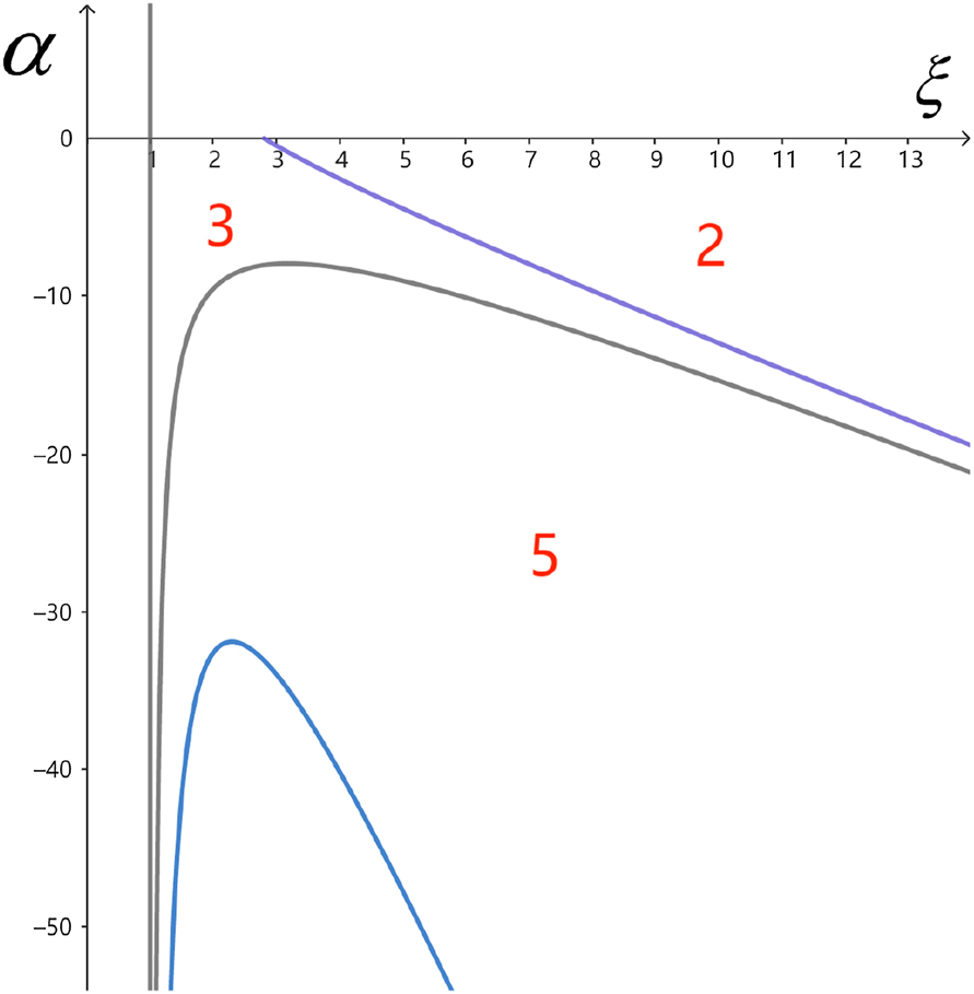
(Sphere case α negative) The subregions of the
We finally are in position to summarize the involved discussion in the following conclusive result for the sphere.
Theorem 3.1.
Under the above notations, the indices of a circular orbit on sphere are given by
A direct consequence of Theorem 3.1 concerns the Morse index of the circular orbits in one physically interesting cases: α = 2 corresponding to a elastic like potential.
Corollary 3.2.
For α = 2, then we get m −(x) = 3.
3.2 Circular orbits on the hyperbolic plane
This subsection is devoted to compute the Morse index for circular orbits on the pseudo-sphere. In this case
We let
By a direct computations we have
Notation 3.3.
Abusing notation, let us now introduce the following notation similar to that of Equation (2.2), we have
Since the (RHS) of the equation defining
By a straightforward computation, we get
Then we have
Similar to the sphere case, we start determining the sign of d ranging in the parameter region
By the explicit computation of d given at Equation (3.10), we infer that the sign of d is minus the sign of
We can check that g 1(ξ) > 0 and consequently there holds d < 0 for all (ξ, α) ∈ Ω3.
Next we have to study the sign of b 2 + cd. By Equation (3.10) and by a direct computation, we get
Now, we observe that since α > 0 and G(ξ 0) > 0, then the sign of b 2 + cd is equal to the sign of the function
So we have following three subregions of Ω3 according to the sign of g 2(ξ).
So, there holds that
In order to compute the index by Lemma 2.4 we have to determine the value of k. Recall that the value of k is determined by
Moreover, by Equation (3.10) we have
Therefore,
Let
Direct computations show that
But it is impossible since the right-hand side of above inequality is negative for ξ ∈ (0, 1). Moreover, we can check that for every fixed α and
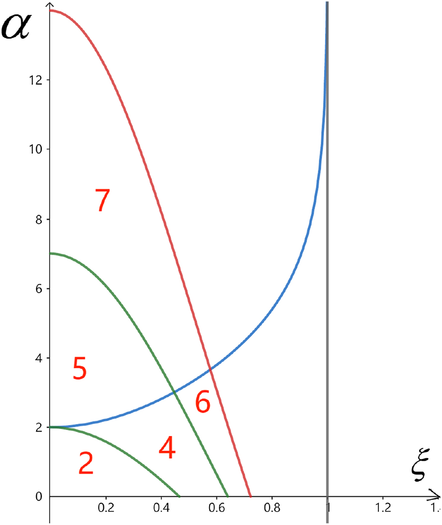
All these subregions are displayed in Figure 5. Invoking Lemma 2.4, then we have the following result.
(Hyperbolic case α positive) In this figure are displayed the subregions of the
Theorem 3.4.
Under the above notations, the Morse index of the circular orbit on the hyperbolic plane is given by
As direct consequence of Theorem 3.4, in the special case of α = 2 we get the following result.
Corollary 3.5.
For α = 2, the Morse index of the circular solution is given by
3.3 Euclidean case
The last case is provided by the Euclidean one. We start letting
and by a direct computation, we get
By Equation (2.2), we get
Since the (RHS) of the equation defining
By a direct computation, we get
By this, we get that the four constants appearing at Equation (2.3) are the following
Now, we observe that d < 0 for all α > 0 and ξ 0 > 0.
Next we need to determine the sign of the term b 2 + cd. By a direct computing we get
By taking into account Equations (3.12) and (3.13) we finally get
Therefore
and we get that k ≥ 1. Indeed, for every
and so on.
Then we have the following result.
Theorem 3.6.
Under the above notations, the Morse index of a circular orbit in the Euclidean plane is given by
By Theorem 3.6 we have the following direct corollary.
Corollary 3.7.
For α = 2, we get
Acknowledgments
The author is grateful for the reviewer’s valuable comments that improved the manuscript.
-
Research ethics: Not applicable.
-
Informed consent: Not applicable.
-
Author contributions: The author confirms the sole responsibility for the conception of the study, presented results and manuscript preparation.
-
Use of Large Language Models, AI and Machine Learning Tools: None declared.
-
Conflict of interest: Author states no conflict of interest.
-
Research funding: The author was supported by Jiangxi Provincial Natural Science Foundation (No. 20232BAB211005), the National Natural Science Foundation of China (Nos. 12001098, 42264007).
-
Data availability: Not applicable.
References
[1] V. V. Kozlov and A. O. Harin, Kepler’s problem in constant curvature spaces, Celestial Mech. Dynam. Astronom. 54 (1992), no. 4, 393–399, https://doi.org/10.1007/BF00049149.Suche in Google Scholar
[2] R. Montgomery, MICZ-Kepler: dynamics on the cone over SO(n), Regul. Chaotic Dyn. 18 (2013), no. 6, 600–607, https://doi.org/10.1134/S1560354713060038.Suche in Google Scholar
[3] F. Diacu, E. Pérez-Chavela, and M. Santoprete, The n-body problem in spaces of constant curvature. Part I: relative equilibria, J. Nonlinear Sci. 22 (2012), no. 2, 247–266, https://doi.org/10.1007/s00332-011-9116-z.Suche in Google Scholar
[4] F. Diacu, E. Pérez-Chavela, and M. Santoprete, The n-body problem in spaces of constant curvature. Part II: singularities, J. Nonlinear Sci. 22 (2012), no. 2, 267–275, https://doi.org/10.1007/s00332-011-9117-y.Suche in Google Scholar
[5] S. Bolotin and V. Kozlov, Topological approach to the generalized n-centre problem, Russ. Math. Surv. 72 (2017), no. 3, 451–478. https://doi.org/10.1070/RM9779.Suche in Google Scholar
[6] S. Baranzini, A. Portaluri, and R. Yang, Morse index of circular solutions for attractive central force problems on surfaces, J. Math. Anal. Appl. 537 (2024), no. 1, 128250, https://doi.org/10.1016/j.jmaa.2024.128250.Suche in Google Scholar
[7] S. Chow, C. Li, and D. Wang, Normal Forms and Bifucations of Planar Vector Fields, Cambridge University Press, Cambridge, 1994.10.1017/CBO9780511665639Suche in Google Scholar
[8] V. I. Arnol’d, On a characteristic class entering into conditions of quantization, (Russian), Funktsional. Anal. i Prilozhen. 1 (1967), 1–14.10.1007/BF01075861Suche in Google Scholar
[9] E. Cappell, R. Lee, and Y. Miller, On the Maslov index, Comm. Pure Appl. Math. 47 (1994), no. 2, 121–186, https://doi.org/10.1002/cpa.3160470202.Suche in Google Scholar
[10] X. Hu and S. Sun, Index and stability of symmetric periodic orbits in Hamiltonian systems with application to figure-eight orbit, Comm. Math. Phys. 290 (2009), no. 2, 737–777, https://doi.org/10.1007/s00220-009-0860-y.Suche in Google Scholar
[11] Y. Long, Index Theory for Symplectic Paths with Applications, Progress in Mathematics, vol. 207, Birkhäuser Verlag, Basel, 2002.10.1007/978-3-0348-8175-3Suche in Google Scholar
[12] Q. Xing, Maslov index for heteroclinic orbits of non-Hamiltonian systems on a two-dimensional phase space, Topol. Methods Nonlinear Anal. 59 (2022), no. 1, 113–130. https://doi.org/10.12775/TMNA.2021.005.Suche in Google Scholar
[13] V. Barutello, R. Jadanza, and A. Portaluri, Morse index and linear stability of the Lagrangian circular orbit in a three-body-type problem via index theory, Arch. Ration. Mech. Anal. 219 (2016), no. 1, 387–444, https://doi.org/10.1007/s00205-015-0898-2.Suche in Google Scholar
[14] H. Kavle, D. Offin, and A. Portaluri, Keplerian orbits through the Conley-Zehnder index, Qual. Theory Dyn. Syst. 20 (2021), no. 10, 10, https://doi.org/10.1007/s12346-020-00430-0.Suche in Google Scholar
[15] Y. Long and T. An, Indexing domains of instability for Hamiltonian systems, NoDEA, Nonlinear Differ. Equ. Appl. 5 (1998), 461–478, https://doi.org/10.1007/s000300050057.Suche in Google Scholar
[16] Y. Long and C. Zhu, Maslov-type index theory for symplectic paths and spectral flow (I), Chin. Ann. Math. Ser. B 20 (1999), no. 4, 413–424, https://doi.org/10.1142/S0252959999000485.Suche in Google Scholar
[17] Y. Long and C. Zhu, Maslov-type index theory for symplectic paths and spectral flow (II), Chin. Ann. Math. Ser. B 21 (2000), no. 1, 89–108, https://doi.org/10.1142/S0252959900000133.Suche in Google Scholar
[18] J. Robbin and D. Salamon, The Maslov index for paths, Topology 32 (1993), no. 4, 827–844, https://doi.org/10.1016/0040-9383(93)90052-W.Suche in Google Scholar
[19] C. Viterbo, Indice de Morse des points critiques obtenus par minimax, Ann. Inst. H. Poincare Anal. Non Linéaire 5 (1998), 221–225. https://doi.org/10.1016/S0294-1449(16)30345-6.Suche in Google Scholar
[20] C. Zhu, A generalized Morse index theorem, Analysis, Geometry and Topology of Elliptic Operators, World Scientific Publishing, Hackensack, NJ, 2006, pp. 493–540.10.1142/9789812773609_0020Suche in Google Scholar
[21] Y. Deng, F. Diacu, and S. Zhu, Variational property of periodic Kepler orbits in constant curvature spaces, J. Differ. Equ. 267 (2019), no. 10, 5851–5869, https://doi.org/10.1016/j.jde.2019.06.008.Suche in Google Scholar
© 2025 the author(s), published by De Gruyter, Berlin/Boston
This work is licensed under the Creative Commons Attribution 4.0 International License.
Artikel in diesem Heft
- On I-convergence of nets of functions in fuzzy metric spaces
- Special Issue on Contemporary Developments in Graphs Defined on Algebraic Structures
- Forbidden subgraphs of TI-power graphs of finite groups
- Finite group with some c#-normal and S-quasinormally embedded subgroups
- Classifying cubic symmetric graphs of order 88p and 88p 2
- Two-sided zero-divisor graphs of orientation-preserving and order-decreasing transformation semigroups
- Simplicial complexes defined on groups
- Further results on permanents of Laplacian matrices of trees
- Algebra
- Classes of modules closed under projective covers
- On the dimension of the algebraic sum of subspaces
- Green's graphs of a semigroup
- On an uncertainty principle for small index subgroups of finite fields
- On a generalization of I-regularity
- Algorithm and linear convergence of the H-spectral radius of weakly irreducible quasi-positive tensors
- The hyperbolic CS decomposition of tensors based on the C-product
- On weakly classical 1-absorbing prime submodules
- Equational characterizations for some subclasses of domains
- Algebraic Geometry
- Spin(8, ℂ)-Higgs bundles fixed points through spectral data
- Embedding of lattices and K3-covers of an Enriques surface
- Kodaira-Spencer maps for elliptic orbispheres as isomorphisms of Frobenius algebras
- Applications in Computer and Information Sciences
- Dynamics of particulate emissions in the presence of autonomous vehicles
- Exploring homotopy with hyperspherical tracking to find complex roots with application to electrical circuits
- Category Theory
- The higher mapping cone axiom
- Combinatorics and Graph Theory
- 𝕮-inverse of graphs and mixed graphs
- On the spectral radius and energy of the degree distance matrix of a connected graph
- Some new bounds on resolvent energy of a graph
- Coloring the vertices of a graph with mutual-visibility property
- Ring graph induced by a ring endomorphism
- A note on the edge general position number of cactus graphs
- Complex Analysis
- Some results on value distribution concerning Hayman's alternative
- Freely quasiconformal and locally weakly quasisymmetric mappings in metric spaces
- A new result for entire functions and their shifts with two shared values
- On a subclass of multivalent functions defined by generalized multiplier transformation
- Singular direction of meromorphic functions with finite logarithmic order
- Growth theorems and coefficient bounds for g-starlike mappings of complex order λ
- Refinements of inequalities on extremal problems of polynomials
- Control Theory and Optimization
- Averaging method in optimal control problems for integro-differential equations
- On superstability of derivations in Banach algebras
- The robust isolated calmness of spectral norm regularized convex matrix optimization problems
- Observability on the classes of non-nilpotent solvable three-dimensional Lie groups
- Differential Equations
- The ill-posedness of the (non-)periodic traveling wave solution for the deformed continuous Heisenberg spin equation
- A note on the global existence and boundedness of an N-dimensional parabolic-elliptic predator-prey system with indirect pursuit-evasion interaction
- Blow-up of solutions for Euler-Bernoulli equation with nonlinear time delay
- Periodic or homoclinic orbit bifurcated from a heteroclinic loop for high-dimensional systems
- Regularity of weak solutions to the 3D stationary tropical climate model
- Local minimizers for the NLS equation with localized nonlinearity on noncompact metric graphs
- Global existence and blow-up of solutions to pseudo-parabolic equation for Baouendi-Grushin operator
- Bubbles clustered inside for almost-critical problems
- Existence and multiplicity of positive solutions for multiparameter periodic systems
- Existence of positive periodic solutions for evolution equations with delay in ordered Banach spaces
- On a nonlinear boundary value problems with impulse action
- Normalized ground-states for the Sobolev critical Kirchhoff equation with at least mass critical growth
- Multiple positive solutions to a p-Kirchhoff equation with logarithmic terms and concave terms
- Infinitely many solutions for a class of Kirchhoff-type equations
- Real and non-real eigenvalues of regular indefinite Sturm–Liouville problems
- Existence of global solutions to a semilinear thermoelastic system in three dimensions
- Limiting profile of positive solutions to heterogeneous elliptic BVPs with nonlinear flux decaying to negative infinity on a portion of the boundary
- Morse index of circular solutions for repulsive central force problems on surfaces
- Differential Geometry
- On tangent bundles of Walker four-manifolds
- Pedal and negative pedal surfaces of framed curves in the Euclidean 3-space
- Discrete Mathematics
- Eventually monotonic solutions of the generalized Fibonacci equations
- Dynamical Systems Ergodic Theory
- Dynamical properties of two-diffusion SIR epidemic model with Markovian switching
- A note on weighted measure-theoretic pressure
- Pullback attractors for a class of second-order delay evolution equations with dispersive and dissipative terms on unbounded domain
- Pullback attractor of the 2D non-autonomous magneto-micropolar fluid equations
- Functional Analysis
- Spectrum boundary domination of semiregularities in Banach algebras
- Approximate multi-Cauchy mappings on certain groupoids
- Investigating the modified UO-iteration process in Banach spaces by a digraph
- Tilings, sub-tilings, and spectral sets on p-adic space
- Continuity and essential norm of operators defined by infinite tridiagonal matrices in weighted Orlicz and l∞ spaces
-
A family of commuting contraction semigroups on
- q-Stirling sequence spaces associated with q-Bell numbers
- Chlodowsky variant of Bernstein-type operators on the domain
- Hyponormality on a weighted Bergman space of an annulus with a general harmonic symbol
- Characterization of derivations on strongly double triangle subspace lattice algebras by local actions
- Fixed point approaches to the stability of Jensen’s functional equation
- Geometry
- The regularity of solutions to the Lp Gauss image problem
- Solving the quartic by conics
- Group Theory
- On a question of permutation groups acting on the power set
- A characterization of the translational hull of a weakly type B semigroup with E-properties
- Harmonic Analysis
- Eigenfunctions on an infinite Schrödinger network
- Maximal function and generalized fractional integral operators on the weighted Orlicz-Lorentz-Morrey spaces
- Subharmonic functions and associated measures in ℝn
- Mathematical Logic, Model Theory and Foundation
- A topology related to implication and upsets on a bounded BCK-algebra
- Boundedness of fractional sublinear operators on weighted grand Herz-Morrey spaces with variable exponents
- Number Theory
- Fibonacci vector and matrix p-norms
- Recurrence for probabilistic extension of Dowling polynomials
- Carmichael numbers composed of Piatetski-Shapiro primes in Beatty sequences
- The number of rational points of some classes of algebraic varieties over finite fields
- Classification and irreducibility of a class of integer polynomials
- Decompositions of the extended Selberg class functions
- Joint approximation of analytic functions by the shifts of Hurwitz zeta-functions in short intervals
- Fibonacci Cartan and Lucas Cartan numbers
- Recurrence relations satisfied by some arithmetic groups
- The hybrid power mean involving the Kloosterman sums and Dedekind sums
- Numerical Methods
- A modified predictor–corrector scheme with graded mesh for numerical solutions of nonlinear Ψ-caputo fractional-order systems
- A kind of univariate improved Shepard-Euler operators
- Probability and Statistics
- Statistical inference and data analysis of the record-based transmuted Burr X model
- Multiple G-Stratonovich integral in G-expectation space
- p-variation and Chung's LIL of sub-bifractional Brownian motion and applications
- Real Analysis
- Chebyshev polynomials of the first kind and the univariate Lommel function: Integral representations
- Multiple solutions for a class of fourth-order elliptic equations with critical growth
- Majorization-type inequalities for (m, M, ψ)-convex functions with applications
- The evaluation of a definite integral by the method of brackets illustrating its flexibility
- Some new Fejér type inequalities for (h, g; α - m)-convex functions
- Some new Hermite-Hadamard type inequalities for product of strongly h-convex functions on ellipsoids and balls
- Topology
- Unraveling chaos: A topological analysis of simplicial homology groups and their foldings
- A generalized fixed-point theorem for set-valued mappings in b-metric spaces
- On SI2-convergence in T0-spaces
- Generalized quandle polynomials and their applications to stuquandles, stuck links, and RNA folding