A note on the edge general position number of cactus graphs
-
Yahan Cao
 and
Shengjin Ji
and
Shengjin Ji


Abstract
For a given graph G, a subset S of E(G) is an edge general position set of G if no triple of S is contained in a common shortest path. The cardinality of a largest edge general position set of G is called the edge general position number of G, denoted by gp e (G). In the paper, sharp upper and lower bounds of the edge general position number are obtained among cactus graphs. Moreover, we characterize all graphs that attained these bounds.
1 Research background
Let G = (V(G), E(G)) be a finite simple graph with vertex set V(G) and edge set E(G). As usual, |V(G)| and |E(G)| are called the order and the size of G, respectively. If uv ∈ E(G), then we say that u is a neighbor of v in G and vice versa. For a vertex v ∈ V(G), set N G (v) = {u ∈ V(G) | uv ∈ E(G)} is regarded as the open neighborhood of v. The degree of a vertex v ∈ V(G) is d G (v) = |N G (v)|. The general position problem in graph theory is to find a largest set of vertices S ⊆ V(G), called a gp-set of G, such that no shortest path of G contains three vertices of S, which was first proposed by Manuel and Klavžar [1]. The general position number (gp-number for short) of G, denoted by gp(G), is the cardinality of a gp-set of G. In fact, they researched the basic properties and the bounds of gp-number in some special graphs, meanwhile, they proved that the general position problem is NP-complete. Note that the classical general position problem is traced back close to the celebrated century-old problem named as the no-three-in-line problem, first introduced by Dudeney [2] in 1917. Recently, Payne and Wood [3] extended the no-three-in-line problem to the general position subset selection problem in discrete geometry. For progress in this regard, see [4],5] and references therein.
Now we focus on the general position problem in graph theory. Patkós [6] studied the gp-number of Kneser graphs, and determined the exact value of gp-number of some special Kneser graphs by using a generalization of Bollobás’s inequality on intersecting set pair systems. Klavžar et al. [7] and Tian and Xu [8] studied the gp-number of Cartesian products. Tian et al. [9] determined the gp-numbers of maximal outerplanar graphs. For further results, see the recent survey on gp-number [10].
The edge general position set of a graph is the edge version of the general position set of a graph, see the seminal paper [11]. We now introduce formally its definition as follows. Let G = (V(G), E(G)) be a graph and S ⊆ E(G). We say that S is an edge general position set if no three edges of S lie on a common shortest path. The subset S is also called a maximum edge general position set if it has the largest cardinality in all edge general position sets. We also call S a gp e -set of G for short. The edge general position number (gp e -number for short) of G, denoted by gp e (G), is the cardinality of a gp e -set in G. An edge general position problem is to find a gp e -set of graphs. And then it should be added that the edge general position set has been recently extended to k-edge general position sets in [12]. Klavžar and Tan [13] obtained the sharp bounds of gp e -number on Fibonacci and Lucas Cubes. Note that many researchers concerned the extremal problems of cactus graphs, cf. [14], [15], [16], [17]. Hence, it is interesting to study the gp e -number of cactus graphs. In the paper, we continue the research in this direction.
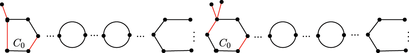
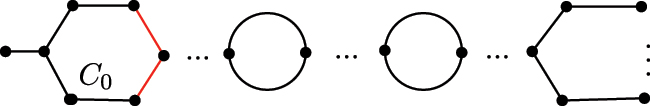
For convenience, we now introduce some notations. A block of G is a maximal connected subgraph of G without cut vertex. A connected graph G is called a cactus graph if its any block is either a cycle or an edge. Let
Let
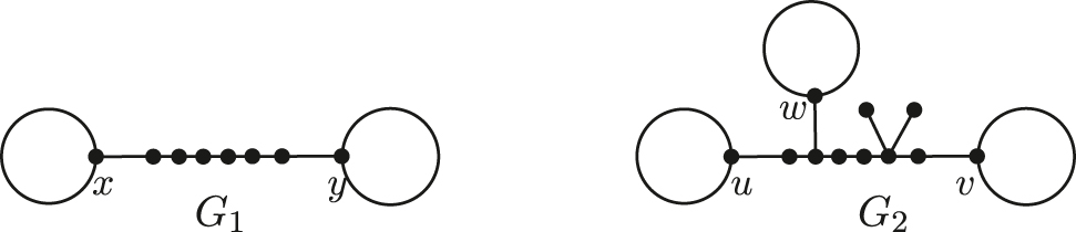
The two examples of cyclic paths.
In the paper, sharp upper and lower bounds of gp e -number are obtained among cactus graphs with k cycles and t pendant leaves. Moreover, we characterize the structures of these graphs that attain the bounds.
2 Edge general position sets of cactus graphs
In the section, we first give some notations which will be useful in showing our main results. We will obtain the upper bound of gp
e
-number in
2.1 Notations
2.1.1 An inner cycle and an outer cycle
We now define several types of cycles of G by means of the cut vertices contained in these cycles. A cycle C l is an inner cycle if there are at least two subgraphs of G − E(C l ) containing cycles, an outer cycle otherwise. In particular, an outer cycle with exactly one cut vertex is an end-block.
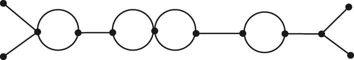
A root chain cactus graph.
2.1.2 A chain cactus and a root chain cactus
A chain cactus G is a cactus graph in which all blocks have at most two cut vertices, and each cut vertex is exactly shared by two blocks. Clearly, a chain graph G has exactly two outer cycles and at most two leaves. We call a graph G′ a root chain cactus if it is obtained from G by changing at least one outer cycle of G such that it contains exactly one root tree with two leaves at a vertex other than the inner cut vertex, see Figure 2. The subgraph of G formed from two outer cycles and the inner cycles and cyclic paths connecting them is called a subchain cactus of G. A subchain cactus of the chain cactus graph presented in Figure 3 is obtained from it by removing two leaves.
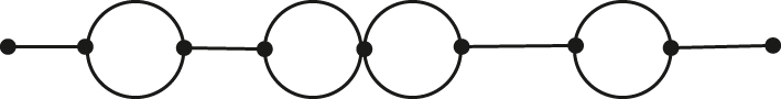
A chain cactus graph.
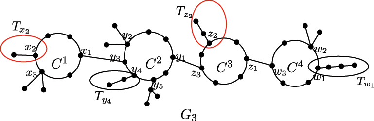
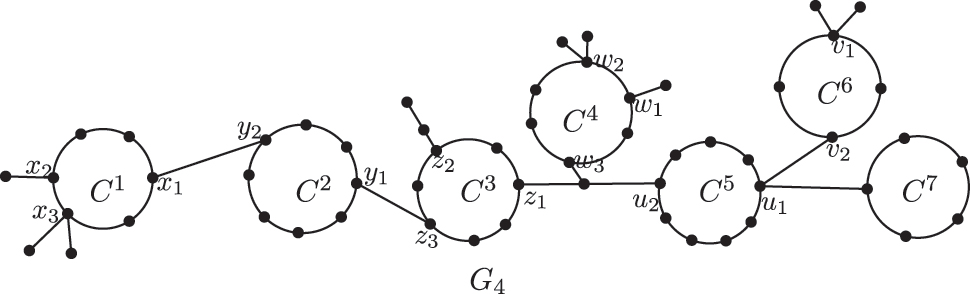
2.1.3 A cut-path of C l and D c (C l )
Let u
i
and u
j
be two vertices of C
l
, clearly, C
l
can be regarded as consisting of two (u
i
, u
j
)-paths. If all cut vertices lying on C
l
belong to one (u
i
, u
j
)-path, then the path is referred to as a (u
i
, u
j
)-cut-path (or a cut-path for short) and then denote d
c
(u
i
, u
j
) the number of edges contained in it, e.g., d
c
(z
1, z
3) = 4 see Figure 4. In particular, suppose now that a cycle C
l
of G has at least three cut vertices. If there are three cut vertices satisfying the following: two cut vertices x
i
and x
j
form a (x
i
, x
j
)-cut-path only containing the third cut vertex x
k
while it is the root vertex of a root tree
Illustrative examples of cut-path, root cut-path and D c .
2.1.4 A good cycle, a normal cycle and a bad cycle
We now give a classification of cycles in G under the assumption that if C
l
is an outer cycle then c(C
l
) ≥ 4. We call the cycle C
l
a normal I cycle if D
c
is no more than
Illustrative examples of different kinds of cycles.
In particular, suppose next that C l is an outer cycle with c(C l ) ≤ 3. For c(C l ) = 1, clearly, C l is an end-block. Then C l is either a normal I cycle for even order, or a good cycle otherwise. Assume now that 2 ≤ c(C l ) ≤ 3.
Let the order of C
l
be even. The cycle C
l
is a normal I cycle with the condition
Suppose the order of C
l
is odd. The cycle C
l
is a normal I cycle if
2.2 The upper bounds of the edge general position number
From [18], we know the following proposition.
Proposition 2.1.
gp e (C n ) = n if n ∈ {3, 4, 5}, and gp e (C n ) = 4 otherwise.
Observation 2.1.
For arbitrary graph
Lemma 2.1.
Let
Proof.
Suppose
Case 1 H 1 and H 2 contain end-blocks.
Let C i be an end-block of H i and u i be the unique cut vertex for i = 1, 2. We first consider that the lengths of C 1 and C 2 have the same parity. If |V(C 1)| and |V(C 2)| are odd, then they are good cycles. From the maximum of S and e ∈ S, we deduce that one of |S ∩ E(C 1)| and |S ∩ E(C 2)| equals 1 and the other equals 3. Without loss of generality, assume that |S ∩ E(C 1)| = 1 and |S ∩ E(C 2)| = 3. Let S 1 = (S − {e}) ∪ {e 1, e 2}, where e 1 and e 2 are two edges incident with u 1 in C 1, as shown in Figure 6. It follows that S 1 is a new edge general position set of G larger than S, a contradiction. If |V(C 1)| and |V(C 2)| are even, then they are normal I cycles. By the choice of S, we obtain that one of |S ∩ E(C 1)| and |S ∩ E(C 2)| equals 0 and the other equals 2. Without loss of generality, assume that |S ∩ E(C 1)| = 0 and |S ∩ E(C 2)| = 2. Let S 2 = (S − {e}) ∪ {e 1, e 2}, where e 1 and e 2 are two edges incident with u 1 in C 1, as shown in Figure 7. Obviously, |S 2| > |S|. In addition, observe that S 2 is also an edge general position set of G, contradicting our assumption. We now assume that the lengths of C 1 and C 2 have different parity. Using the similar way of the first case, we also have done. So we omit the process here.
Case 2 H 1 and H 2 contain no end-blocks.
Assume that
We now consider that S ∩ L
1 = ∅ and S ∩ L
2 = ∅ hold simultaneously. So we deduce that
Case 3 One of H 1 and H 2 contains end-blocks.
Assume that H 1 contains an end-block, denoted by C 3. Let u 3 be the inner cut vertex in C 3. Then C 3 is a normal I cycle for even order or a good cycle otherwise. Let C 4 be an outer cycle in H 2 and L 3 be the set of pendant edges belonging to root trees of C 4. Then one of S ∩ L 3 = ∅ and S ∩ L 3 ≠ ∅ holds. For each case, the choice of S and e ∈ S imply that |S ∩ C 3| ∈ {0, 1}. Let S 3 = (S − {e}) ∪ {e 31, e 32} with |S 3| > |S|, where e 31 and e 32 incident with u 3 of C 3. It follows that S 3 is also an edge general position set of G, a contradiction.
Therefore, we finish the proof.□
Used to illustrate Case 1, both C 1 and C 2 are odd cycles.
Used to illustrate Case 1, both C 1 and C 2 are even cycles.
Lemma 2.2.
Suppose
(i) |E(C 0) ∩ S| = 3 if and only if C 0 is a good cycle.
(ii) |E(C 0) ∩ S| = 2 if and only if C 0 is a normal I cycle or a normal II cycle.
(iii) |E(C 0) ∩ S| = 0 if and only if C 0 is a bad cycle.
Proof.
Let G be a cactus graph with k ≥ 2 cycles and t leaves. Let S be a gp e -set containing pendant edges and these edges from outer cycles as more as possible. By means of Lemma 2.1, the elements of S are derived from cycles and root trees of G. Assume that C 0 is a cycle of G. We first prove the following claim.□
Claim 1. |S ∩ E(C 0)| ≤ 3.
Proof.
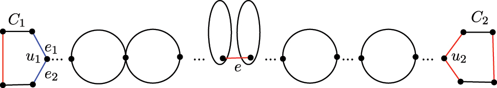
By contradiction, suppose |S ∩ E(C 0)| ≥ 4. Together with Proposition 2.1, we conclude that |S| = |S ∩ E(C 0)| ∈ {4, 5}.
If C
0 is an inner cycle, then we deduce that G is a chain cactus by the maximum of S. Assume that C
1 and C
2 are two outer cycles of G with two inner cut vertices u
1 and u
2, respectively. In addition, by the choice of S, |S ∩ E(C
i
)| = 0 for i = 1, 2. Clearly, C
0 is an even cycle. Otherwise,
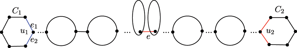
If C
0 is an outer cycle with the inner cut vertex u
0, then by the choice of S we have that G is a chain cactus graph. In other words, all inner cycles are bad. Let
Hence, |S ∩ E(C 0)| ≤ 3 is true.□
We now divide the following cases to finish the remaining proof.
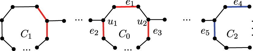
Case 1 C 0 is an inner cycle of G.
In the case, we know that k ≥ 3. Note that, for each inner cycle C
0, there are two outer cycles C
1 and C
2 of G for which C
0 is lying on its unique subchain cactus between C
1 and C
2. Let u
1 and u
2 be the two inner cut vertices of C
0 belonging to the subchain cactus. By the maximum of S, we can claim that |S ∩ E(C
0)| ≤ 2. Assume to the contrary that |S ∩ E(C
0)| ≥ 3. Recall that |S ∩ E(C
0)| ≤ 3. So |S ∩ E(C
0)| = 3. Set {e
1, e
2, e
3} ⊆ S ∩ E(C
0). So there exists an edge, say e
1, such that it lies on a (u
1, u
2)-path with length no more than
Used to illustrate Case 1.
Observe that, if
Case 2 C 0 is an outer cycle of G.
Note that c(C 0) ≥ 1. Assume now that c(C 0) = 1, which implies that C 0 is an end-block. The choice of S results in either |S ∩ E(C 0)| = 3 for odd order or |S ∩ E(C 0)| = 2 for even order.
We now assume that c(C
0) ≥ 4. According to the values of D
c
(C
0), we conclude that |S ∩ E(C
0)| = 2 with
Assume next that c(C
0) = 3. By the values of D
c
(C
0), we deduce that |S ∩ E(C
0)| = 2 with
We now consider the case c(C
0) = 2. It is clear that
Used to illustrate Case 2 with c(C 0) = 2 and C 0 is a normal I cycle.

Used to illustrate Case 2 with c(C 0) = 2 and C 0 is a bad cycle.
Used to illustrate Case 2 with c(C 0) = 2 and C 0 is a normal II cycle.
Therefore, we have done as required. □
Based on the above conclusions, we deduce the following result.
Theorem 2.1.
For k ≥ 2, let
Proof.
Suppose that
Hence, we next show the second part of the conclusion. Assume now that G is a cactus graph such that gp e (G) = |S| = 2(k − r) + 3r + t. From Lemma 2.2, we have that |S ∩ E(C l )| ≤ 3, and then, |S ∩ E(C l )| ≤ 2 for even l. We first claim that each odd cycle C l is an end-block. If it is not an end-block, then |S ∩ E(C l )| ≤ 2 by Lemma 2.2. So we get that.
a contradiction. We next claim that each even cycle C l is a normal I cycle. Contrary to our claim, suppose that C l is not normal I. Hence, C l is either a normal II cycle or a bad cycle. From by Lemma 2.2, we deduce that either |S| ≤ ≤ 2 + 2(k − r) + 3(r − 1) + t − 1 < 2(k − r) + 3r + t for the first case, or |S| ≤ ≤ 0 + 2(k − r) + 3(r − 1) + t < 2(k − r) + 3r + t otherwise. We get a contradiction.
Combining the above two cases, |S| = 2(k − r) + 3r + t implies that G contains r good odd cycle and k − r even normal I cycle. In other words, all root trees are lying on cut-paths with length less than a half of the order of each even cycle. Consequently,
The following two results hold directly from Theorem 2.1.
Corollary 2.2.
Let
Corollary 2.3.
Suppose that
Theorem 2.4.
Let
where equality holds if and only if all cycles of G are good odd cycles.
Proof.
Suppose that
Case 1 k = 1 and t ≤ 1.
In fact, G is a unicyclic graph with a unique cycle C l . Clearly, 3k + t ≤ 4 < 5. It is easy to check that gp e (G) ≤ 5 with equality holds if and only if G ≅ C 5. At the time, C 5 is a good odd cycle of G.
Case 2 k = 1 and t ≥ 2.
Note that C l is a unique cycle of G. In addition, 5 ≤ 3k + t. By direct checking, we obtain that gp e (G) ≤ 3k + t with equality if and only if the length of C l is odd and C l has a unique root tree with t leaves. So C l is a good odd cycle.
Case 3 k ≥ 2.
Observe that 5 < 3k + t. Meanwhile, from Corollary 2.2, we obtain gp e (G) ≤ 3k + t with equality only if G contains k good odd cycles.□
2.3 The lower bounds of the edge general position number
Note that if a chain cactus G has two even end-blocks and its every inner cycle is bad and has two cut vertices, then gp e (G) = 4, as an example G ≅ G k see Figure 12. The graph G k also appeared in [18], Figure 2]. Observe that a cactus graph G with at least two outer cycles has gp e (G) ≥ 4. In addition, if G has t leaves, then there is an edge general position set of G consisting of t pendant edges. It follows that gp e (G) ≥ t. Observe that gp e (G k,t ) = t, where G k,t contains k − 2 triangles, 2 C 4 and t leaves such that each cycle has at least two leaves, as shown in Figure 12. Are they the lower bounds of the cactus graphs? In the following subsection, we will confirm the observations and obtain two sharp lower bounds of the cactus graphs.
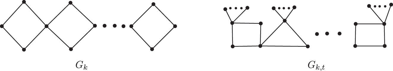
Two examples used in Theorems 2.5 and 2.6.
Theorem 2.5.
Let
Proof.
Let
Case 1 |S ∩ L| = t − 1.
From the assumption, we know that all outer cycles of G are not end-block. Assume that e 1 is the unique pendant edge with e 1 ∈ (L − S) and e 2 is the unique edge with e 2 ∈ (S − L). If e 1 and e 2 are lying on the same pendant path of G, then S′ = (S − e 2) ∪ {e 1} is also a gp e -set of G. We get a contradiction with the choice of S. Hence, e 2 is one edge of some cycle in G. Clearly, e 2 belongs to a normal I cycle or a normal II cycle. (Otherwise, it is contained in some outer cycle, it follows that G has a bigger edge general position set S ∪ {e 1}, a contradiction.) By Lemma 2.2, we also get a contradiction with the choice of S.
Case 2 |S ∩ L| ≤ t − 2.
Let e 1 and e 2 be two pendant edges not contained in S. From Case 1, we can assume that the edges in S that are not pendant edges lie on cycles. Let e 3 and e 4 be two elements of S not contained in L. The strategy of choosing these two edges is to make them come from the same cycle as much as possible. We can assume that e 3 and e 4 are contained in some cycle by Case 1. Hence, the cycle is either an outer cycle or an inner cycle of G, say C 0. So, from Lemma 2.2 we get a contradiction to the choice of S. Therefore, we confirm that S = L. Together with Lemma 2.2, we deduce that all cycles of G are bad.□
Theorem 2.6.
If
Proof.
Let
Case 1 Outer cycles contain no root trees.
By our assumption, each outer cycle of G is an end-block. Hence, G is a chain cactus with two even end-blocks. Otherwise, gp e (G) ≥ 5 by Lemma 2.2, a contradiction. Evidently, S contains four proper edges from two end-blocks. Recall that |S| = 4, which infers that all inner cycles contribute 0 edge to S. By Lemma 2.2, all inner cycles are bad and even.
Case 2 An outer cycle contains a root tree, say T.
Observe that T has at most 2 leaves. We first claim that all inner cycles are bad. Otherwise, there is an inner cycle which contributes two edges to S by Lemma 2.2. Together with proper four edges in two outer cycles, we get |S| ≥ 6, a contradiction. Hence, the four edges of S are derived from the two outer cycles, where one outer cycle, denoted by C 0, has the root tree T. Mark the root of T as u′ and the inner cut vertex of C 0 as v 0. We can deduce that u′ and v 0 are diagonal of C 0.
Case 3 An outer cycle contains two root trees, denoted by T 1 and T 2.
Let C 0 be the outer cycle. Let v 1 and v 2 be the roots of T 1 and T 2, and let v 3 be the inner cut vertex of C 0. Using the same argument as in Case 1, we deduce that all inner cycles of G are bad. Observe that T 1 and T 2 are pendant paths by the minimality of S. We find that C 0 is a normal II cycle by the three cut vertices v 1, v 2 and v 3. But we can get another edge general position set with size larger than |S|, a contradiction.
Combining the above three cases, the conclusion is verified.□
3 Conclusions
As we know, the topological indices and other graph invariants have been explored on cactus graphs. In this paper, we research the edge general position number of cactus graphs, and bound it with the number of cycles and pendant vertices. Moreover, we obtain the lower bound and the upper bound by means of the number of good cycles, bad cycles and pendant vertices. We think that determining the formula of the edge general position number of cactus graphs regarding the number of cycles and pendant vertices is an interesting work in the future.
Acknowledgments
The authors would like to thank the editor and referees for their valuable suggestions which helps us to modify the presentation of the paper.
-
Research ethics: Not applicable.
-
Informed consent: Not applicable.
-
Author contributions: Authors have accepted responsibility for the entire content of this manuscript and consented to its submission to the journal, reviewed all the results and approved the final version of the manuscript.
-
Use of Large Language Models, AI and Machine Learning Tools: None declared.
-
Conflict of interest: Authors state no conflicts of interest.
-
Research funding: This work was supported by the Natural Science Foundation of Shandong Province, China (No. ZR2022MA077) and by Postgraduate Education Reform Project of Shandong Province, China (No. SDYKC2023107).
-
Data availability: Data sharing does not apply to this article as no datasets were generated or analysed during the current study.
References
[1] P. Manuel and S. Klavžar, A general position problem in graph theory, Bull. Aust. Math. Soc. 98 (2018), no. 2, 177–187, https://doi.org/10.1017/S0004972718000473.Search in Google Scholar
[2] H. Dudeney, Amusements in Mathematics, Nelson, Edinburgh, 1917.Search in Google Scholar
[3] M. Payne and D. R. Wood, On the general position subset selection problem, SIAM J. Discrete Math. 27 (2013), no. 4, 1727–1733, https://doi.org/10.1137/120897493.Search in Google Scholar
[4] V. Froese, I. Kanj, A. Nichterlein, and R. Niedermeier, Finding points in general position, Int. J. Comput. Geom. Appl. 27 (2017), no. 04, 277–296, https://doi.org/10.1142/S021819591750008X.Search in Google Scholar
[5] A. Misiak, Z. Stępień, A. Szymaszkiewicz, L. Szymaszkiewicz, and M. Zwierzchowski, A note on the no-three-in-line problem on a torus, Discrete Math. 339 (2016), no. 1, 217–221, https://doi.org/10.1016/j.disc.2015.08.006.Search in Google Scholar
[6] B. Patkós, On the general position problem on Kneser graphs, Ars. Math. Contemp. 18 (2020), 273–280, https://doi.org/10.26493/1855-3974.1957.a0f.Search in Google Scholar
[7] S. Klavžar, B. Patkós, G. Rus, and I. G. Yero, On general position sets in Cartesian products, Results Math. 76 (2021), no. 3, 123, https://doi.org/10.1007/s00025-021-01438-x.Search in Google Scholar
[8] J. Tian and K. Xu, The general position number of Cartesian products involving a factor with small diameter, Appl. Math. Comput. 403 (2021), 126206, https://doi.org/10.1016/j.amc.2021.126206.Search in Google Scholar
[9] J. Tian, K. Xu, and D. Chao, On the general position numbers of maximal outerplanar graphs, Bull. Malays. Math. Sci. Soc. 46 (2023), 198, https://doi.org/10.1007/s40840-023-01592-1.Search in Google Scholar
[10] U. S. V. Chandran, S. Klavžar, and J. Tuite, The general position problem: a survey (2025), arXiv:2501.19385, https://doi.org/10.48550/arXiv.2501.19385.Search in Google Scholar
[11] P. Manuel, R. Prabha, and S. Klavžar, The edge general position problem, Bull. Malays. Math. Sci. Soc. 45 (2022), no. 6, 2997–3009, https://doi.org/10.1007/s40840-022-01319-8.Search in Google Scholar
[12] P. Manuel, R. Prabha, and S. Klavžar, Generalization of edge general position problem, Art Discrete Appl. Math. 8 (2024), #P1.02, https://doi.org/10.26493/2590-9770.1745.5f4.Search in Google Scholar
[13] S. Klavžar and E. Tan, Edge general position sets in Fibonacci and Lucas cubes, Bull. Malays. Math. Sci. Soc. 46 (2023), no. 4, 120, https://doi.org/10.1007/s40840-023-01517-y.Search in Google Scholar
[14] I. Gutman, S. Li, and W. Wei, Cacti with n-vertices and t cycles having extremal Wiener index, Discrete Appl. Math. 232 (2017), 189–200, https://doi.org/10.1016/j.dam.2017.07.023.Search in Google Scholar
[15] J. Li, K. Xu, T. Zhang, H. Wang, and S. Wagner, Maximum number of subtrees in cacti and block graphs, Aequationes Math. 96 (2022), no. 5, 1027–1040, https://doi.org/10.1007/s00010-022-00879-1.Search in Google Scholar
[16] Y. Yao, M. He, and S. Ji, On the general position number of two classes of graphs, Open. Math. 20 (2022), no. 1, 1021–1029, https://doi.org/10.1515/math-2022-0444.Search in Google Scholar
[17] S. Wang, On extremal cacti with respect to the Szeged index, Appl. Math. Comput. 309 (2017), 8592, https://doi.org/10.1016/j.amc.2017.03.036.Search in Google Scholar
[18] J. Tian, S. Klavžar, and E. Tan, Extremal edge general position sets in some graphs, Graphs Combin. 40 (2024), no. 2, 40, https://doi.org/10.1007/s00373-024-02770-z.Search in Google Scholar
© 2025 the author(s), published by De Gruyter, Berlin/Boston
This work is licensed under the Creative Commons Attribution 4.0 International License.
Articles in the same Issue
- On I-convergence of nets of functions in fuzzy metric spaces
- Special Issue on Contemporary Developments in Graphs Defined on Algebraic Structures
- Forbidden subgraphs of TI-power graphs of finite groups
- Finite group with some c#-normal and S-quasinormally embedded subgroups
- Classifying cubic symmetric graphs of order 88p and 88p 2
- Two-sided zero-divisor graphs of orientation-preserving and order-decreasing transformation semigroups
- Simplicial complexes defined on groups
- Further results on permanents of Laplacian matrices of trees
- Algebra
- Classes of modules closed under projective covers
- On the dimension of the algebraic sum of subspaces
- Green's graphs of a semigroup
- On an uncertainty principle for small index subgroups of finite fields
- On a generalization of I-regularity
- Algorithm and linear convergence of the H-spectral radius of weakly irreducible quasi-positive tensors
- The hyperbolic CS decomposition of tensors based on the C-product
- On weakly classical 1-absorbing prime submodules
- Equational characterizations for some subclasses of domains
- Algebraic Geometry
- Spin(8, ℂ)-Higgs bundles fixed points through spectral data
- Embedding of lattices and K3-covers of an Enriques surface
- Kodaira-Spencer maps for elliptic orbispheres as isomorphisms of Frobenius algebras
- Applications in Computer and Information Sciences
- Dynamics of particulate emissions in the presence of autonomous vehicles
- Exploring homotopy with hyperspherical tracking to find complex roots with application to electrical circuits
- Category Theory
- The higher mapping cone axiom
- Combinatorics and Graph Theory
- 𝕮-inverse of graphs and mixed graphs
- On the spectral radius and energy of the degree distance matrix of a connected graph
- Some new bounds on resolvent energy of a graph
- Coloring the vertices of a graph with mutual-visibility property
- Ring graph induced by a ring endomorphism
- A note on the edge general position number of cactus graphs
- Complex Analysis
- Some results on value distribution concerning Hayman's alternative
- Freely quasiconformal and locally weakly quasisymmetric mappings in metric spaces
- A new result for entire functions and their shifts with two shared values
- On a subclass of multivalent functions defined by generalized multiplier transformation
- Singular direction of meromorphic functions with finite logarithmic order
- Growth theorems and coefficient bounds for g-starlike mappings of complex order λ
- Refinements of inequalities on extremal problems of polynomials
- Control Theory and Optimization
- Averaging method in optimal control problems for integro-differential equations
- On superstability of derivations in Banach algebras
- The robust isolated calmness of spectral norm regularized convex matrix optimization problems
- Observability on the classes of non-nilpotent solvable three-dimensional Lie groups
- Differential Equations
- The ill-posedness of the (non-)periodic traveling wave solution for the deformed continuous Heisenberg spin equation
- A note on the global existence and boundedness of an N-dimensional parabolic-elliptic predator-prey system with indirect pursuit-evasion interaction
- Blow-up of solutions for Euler-Bernoulli equation with nonlinear time delay
- Periodic or homoclinic orbit bifurcated from a heteroclinic loop for high-dimensional systems
- Regularity of weak solutions to the 3D stationary tropical climate model
- Local minimizers for the NLS equation with localized nonlinearity on noncompact metric graphs
- Global existence and blow-up of solutions to pseudo-parabolic equation for Baouendi-Grushin operator
- Bubbles clustered inside for almost-critical problems
- Existence and multiplicity of positive solutions for multiparameter periodic systems
- Existence of positive periodic solutions for evolution equations with delay in ordered Banach spaces
- On a nonlinear boundary value problems with impulse action
- Normalized ground-states for the Sobolev critical Kirchhoff equation with at least mass critical growth
- Multiple positive solutions to a p-Kirchhoff equation with logarithmic terms and concave terms
- Infinitely many solutions for a class of Kirchhoff-type equations
- Real and non-real eigenvalues of regular indefinite Sturm–Liouville problems
- Existence of global solutions to a semilinear thermoelastic system in three dimensions
- Limiting profile of positive solutions to heterogeneous elliptic BVPs with nonlinear flux decaying to negative infinity on a portion of the boundary
- Morse index of circular solutions for repulsive central force problems on surfaces
- Differential Geometry
- On tangent bundles of Walker four-manifolds
- Pedal and negative pedal surfaces of framed curves in the Euclidean 3-space
- Discrete Mathematics
- Eventually monotonic solutions of the generalized Fibonacci equations
- Dynamical Systems Ergodic Theory
- Dynamical properties of two-diffusion SIR epidemic model with Markovian switching
- A note on weighted measure-theoretic pressure
- Pullback attractors for a class of second-order delay evolution equations with dispersive and dissipative terms on unbounded domain
- Pullback attractor of the 2D non-autonomous magneto-micropolar fluid equations
- Functional Analysis
- Spectrum boundary domination of semiregularities in Banach algebras
- Approximate multi-Cauchy mappings on certain groupoids
- Investigating the modified UO-iteration process in Banach spaces by a digraph
- Tilings, sub-tilings, and spectral sets on p-adic space
- Continuity and essential norm of operators defined by infinite tridiagonal matrices in weighted Orlicz and l∞ spaces
-
A family of commuting contraction semigroups on
- q-Stirling sequence spaces associated with q-Bell numbers
- Chlodowsky variant of Bernstein-type operators on the domain
- Hyponormality on a weighted Bergman space of an annulus with a general harmonic symbol
- Characterization of derivations on strongly double triangle subspace lattice algebras by local actions
- Fixed point approaches to the stability of Jensen’s functional equation
- Geometry
- The regularity of solutions to the Lp Gauss image problem
- Solving the quartic by conics
- Group Theory
- On a question of permutation groups acting on the power set
- A characterization of the translational hull of a weakly type B semigroup with E-properties
- Harmonic Analysis
- Eigenfunctions on an infinite Schrödinger network
- Maximal function and generalized fractional integral operators on the weighted Orlicz-Lorentz-Morrey spaces
- Subharmonic functions and associated measures in ℝn
- Mathematical Logic, Model Theory and Foundation
- A topology related to implication and upsets on a bounded BCK-algebra
- Boundedness of fractional sublinear operators on weighted grand Herz-Morrey spaces with variable exponents
- Number Theory
- Fibonacci vector and matrix p-norms
- Recurrence for probabilistic extension of Dowling polynomials
- Carmichael numbers composed of Piatetski-Shapiro primes in Beatty sequences
- The number of rational points of some classes of algebraic varieties over finite fields
- Classification and irreducibility of a class of integer polynomials
- Decompositions of the extended Selberg class functions
- Joint approximation of analytic functions by the shifts of Hurwitz zeta-functions in short intervals
- Fibonacci Cartan and Lucas Cartan numbers
- Recurrence relations satisfied by some arithmetic groups
- The hybrid power mean involving the Kloosterman sums and Dedekind sums
- Numerical Methods
- A modified predictor–corrector scheme with graded mesh for numerical solutions of nonlinear Ψ-caputo fractional-order systems
- A kind of univariate improved Shepard-Euler operators
- Probability and Statistics
- Statistical inference and data analysis of the record-based transmuted Burr X model
- Multiple G-Stratonovich integral in G-expectation space
- p-variation and Chung's LIL of sub-bifractional Brownian motion and applications
- Real Analysis
- Chebyshev polynomials of the first kind and the univariate Lommel function: Integral representations
- Multiple solutions for a class of fourth-order elliptic equations with critical growth
- Majorization-type inequalities for (m, M, ψ)-convex functions with applications
- The evaluation of a definite integral by the method of brackets illustrating its flexibility
- Some new Fejér type inequalities for (h, g; α - m)-convex functions
- Some new Hermite-Hadamard type inequalities for product of strongly h-convex functions on ellipsoids and balls
- Topology
- Unraveling chaos: A topological analysis of simplicial homology groups and their foldings
- A generalized fixed-point theorem for set-valued mappings in b-metric spaces
- On SI2-convergence in T0-spaces
- Generalized quandle polynomials and their applications to stuquandles, stuck links, and RNA folding