On the δ-chromatic numbers of the Cartesian products of graphs
-
Wipawee Tangjai


Abstract
In this work, we study the
1 Introduction
The concept of
In 1957, Sabidussi [3] showed that the chromatic number of the Cartesian product graphs is equal to the maximum chromatic number between such two graphs. A lot of subsequent research has been exploring different types of chromatic numbers of the Cartesian product graphs such as list chromatic number [4], packing chromatic number [5], and
We first recall some basic notations and definitions needed in this article. Let
In this work, we give a structure of the
2 Preliminary results
In this section, we provide the definitions of the
Definition 1
[1] The
The

Graph
Definition 2
[2] A
Results on the
Theorem 3
[3] Let G and H be graphs. We have
Some Nordhaus-Gaddum bounds on
Theorem 4
[2] For
and
3 Structure of the
δ
-complements of Cartesian products
This section contains the structure of the
The following theorem shows that the edge set of the
Theorem 5
For graphs G and H, we have
Proof
We want to show that
In case
In case
Corollary 6
Let G and H be graphs. We have
The following example illustrates the structure described in Theorem 5.
Example 7
Consider
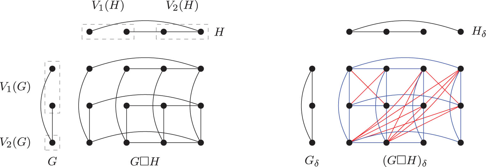
Left: Graph
In general, we have the following theorem for a finite Cartesian product of graphs.
Theorem 8
For graphs
Proof
It is well-known that two vertices
The following two results are applications of Theorem 8.
Theorem 9
Proof
From Theorem 8, we need to show that
Suppose that there are
The converse is obvious.□
Corollary 10
4 Bounds on the
δ
-chromatic numbers of Cartesian products
This section contains our results on lower bounds and upper bounds of
Theorem 11
Let
Proof
The proof follows directly from Theorems 3 and 8.□
The next result gives an upper bound on a Cartesian product of a class of graphs. This result will be used throughout the remaining of this article. The range of the values for the modulo
Theorem 12
Let G and H be graphs. If any positive degree difference of vertices in G is not equal to that of in H, then
where
Proof
By Theorem 5 and the assumption that any positive degree difference of vertices in
Define
for
Finally, any endpoints of an edge in
An example of a coloring in the proof of Theorem 12 where
|
|
|
|
|
|
|
|
|
|---|---|---|---|---|---|---|---|
|
|
1 | 5 | 2 | 3 | 7 | 4 | 8 |
|
|
3 | 7 | 4 | 1 | 5 | 2 | 6 |
|
|
1 | 5 | 2 | 3 | 7 | 4 | 8 |
|
|
2 | 6 | 3 | 4 | 8 | 1 | 5 |
|
|
3 | 7 | 4 | 1 | 5 | 2 | 6 |
Corollary 13
Let G be a graph with
The following theorem implies that the bound given in Theorem 12 is sharp.
Theorem 14
For
Proof
Let
As an example, we apply Theorem 12 to the Cartesian product of a star and a path.
Example 15
For
Proof
Let
The bound in Example 15 is not sharp. When
Theorem 16
Let H be a k-regular graph. Let
Proof
Let
Let
The sharpness of the bound in Theorem 16 will be shown in Theorem 18.
5
δ
-chromatic numbers of the Cartesian products of some graphs
In this section, we give our results on the exact values of the
Theorem 17
Proof
Let
as shown in Figure 3. In addition, the set

A proper
Theorem 18
Proof
Let
When
When
When
as shown in Figure 4. We thus have a proper

A proper
The following lemma is crucial for proving Theorem 20.
Lemma 19
For
Proof
Suppose
Case 1.
Case 2.
Case 3.
The proof of this case is similar to Case 2.
Case 4.
Therefore,
Theorem 20
For
Proof
Let
if
if
We note that
We color
as shown in Figure 5.
The coloring

A proper 10-coloring of
6 Conclusion
In this work, we give a structure of
Acknowledgement
The authors are grateful to Rasimate Maungchang and the reviewers for their valuable comments that improved the manuscript.
-
Funding information: This research project was financially supported by Mahasarakham University.
-
Author contributions: All authors have accepted responsibility for the entire content of this manuscript and consented to its submission to the journal, reviewed all the results, and approved the final version of the manuscript. WT and PV initiated the project. WT, WP, and PV designed, investigated and proved the results. WT, WP, and PV prepared, reviewed, and edited the manuscript. WT and PV administered the project. All authors have read and agreed to the published version of the manuscript.
-
Conflict of interest: The authors state no conflict of interest.
References
[1] A. Pai, H. A. Rao, S. DaSouza, P. G. Bhat, and S. Upadhyay, δ-complement of a graph, Mathematics 10 (2022), no. 8, 1203. 10.3390/math10081203Search in Google Scholar
[2] P. Vichitkunakorn, R. Maungchang, and W. Tangjai, On nordhaus-gaddum type relations of δ-complement graphs, Heliyon 9 (2023), no. 6, e16630. 10.1016/j.heliyon.2023.e16630Search in Google Scholar PubMed PubMed Central
[3] G. Sabidussi, Graphs with given group and given graph-theoretical properties, Canad. J. Math. 9 (1957), 515–525. 10.4153/CJM-1957-060-7Search in Google Scholar
[4] M. Borowiecki, S. Jendrol, D. Král, and J. Missskuf, List coloring of Cartesian products of graphs, Discrete Math. 306 (2006), no. 16, 1955–1958. 10.1016/j.disc.2006.03.062Search in Google Scholar
[5] B. Brešar, S. Klavžar, and D. F. Rall, On the packing chromatic number of Cartesian products, hexagonal lattice, and trees, Discrete Appl. Math. 155 (2007), no. 17, 2303–2311. 10.1016/j.dam.2007.06.008Search in Google Scholar
[6] R. Balakrishnan, S. F. Raj, and T. Kavaskar, b-chromatic number of Cartesian product of some families of graphs, Graphs Combin. 30 (2014), 511–520. 10.1007/s00373-013-1285-0Search in Google Scholar
[7] C. Guo and M. Newman, On the b-chromatic number of Cartesian products, Discrete Appl. Math. 239 (2018), 82–93. 10.1016/j.dam.2017.12.025Search in Google Scholar
© 2024 the author(s), published by De Gruyter
This work is licensed under the Creative Commons Attribution 4.0 International License.
Articles in the same Issue
- Special Issue on Contemporary Developments in Graph Topological Indices
- On the maximum atom-bond sum-connectivity index of graphs
- Upper bounds for the global cyclicity index
- Zagreb connection indices on polyomino chains and random polyomino chains
- On the multiplicative sum Zagreb index of molecular graphs
- The minimum matching energy of unicyclic graphs with fixed number of vertices of degree two
- Special Issue on Convex Analysis and Applications - Part I
- Weighted Hermite-Hadamard-type inequalities without any symmetry condition on the weight function
- Scattering threshold for the focusing energy-critical generalized Hartree equation
- (p, q)-Compactness in spaces of holomorphic mappings
- Characterizations of minimal elements of upper support with applications in minimizing DC functions
- Some new Hermite-Hadamard-type inequalities for strongly h-convex functions on co-ordinates
- Global existence and extinction for a fast diffusion p-Laplace equation with logarithmic nonlinearity and special medium void
- Extension of Fejér's inequality to the class of sub-biharmonic functions
- On sup- and inf-attaining functionals
- Regularization method and a posteriori error estimates for the two membranes problem
- Rapid Communication
- Note on quasivarieties generated by finite pointed abelian groups
- Review Articles
- Amitsur's theorem, semicentral idempotents, and additively idempotent semirings
- A comprehensive review of the recent numerical methods for solving FPDEs
- On an Oberbeck-Boussinesq model relating to the motion of a viscous fluid subject to heating
- Pullback and uniform exponential attractors for non-autonomous Oregonator systems
- Regular Articles
- On certain functional equation related to derivations
- The product of a quartic and a sextic number cannot be octic
- Combined system of additive functional equations in Banach algebras
- Enhanced Young-type inequalities utilizing Kantorovich approach for semidefinite matrices
- Local and global solvability for the Boussinesq system in Besov spaces
- Construction of 4 x 4 symmetric stochastic matrices with given spectra
- A conjecture of Mallows and Sloane with the universal denominator of Hilbert series
- The uniqueness of expression for generalized quadratic matrices
- On the generalized exponential sums and their fourth power mean
- Infinitely many solutions for Schrödinger equations with Hardy potential and Berestycki-Lions conditions
- Computing the determinant of a signed graph
- Two results on the value distribution of meromorphic functions
- Zariski topology on the secondary-like spectrum of a module
- On deferred f-statistical convergence for double sequences
-
About
- Strong convergence for weighted sums of (α, β)-mixing random variables and application to simple linear EV regression model
- On the distribution of powered numbers
- Almost periodic dynamics for a delayed differential neoclassical growth model with discontinuous control strategy
- A new distributionally robust reward-risk model for portfolio optimization
- Asymptotic behavior of solutions of a viscoelastic Shear beam model with no rotary inertia: General and optimal decay results
- Silting modules over a class of Morita rings
- Non-oscillation of linear differential equations with coefficients containing powers of natural logarithm
- Mutually unbiased bases via complex projective trigonometry
- Hyers-Ulam stability of a nonlinear partial integro-differential equation of order three
- On second-order linear Stieltjes differential equations with non-constant coefficients
- Complex dynamics of a nonlinear discrete predator-prey system with Allee effect
- The fibering method approach for a Schrödinger-Poisson system with p-Laplacian in bounded domains
- On discrete inequalities for some classes of sequences
- Boundary value problems for integro-differential and singular higher-order differential equations
- Existence and properties of soliton solution for the quasilinear Schrödinger system
- Hermite-Hadamard-type inequalities for generalized trigonometrically and hyperbolic ρ-convex functions in two dimension
- Endpoint boundedness of toroidal pseudo-differential operators
- Matrix stretching
- A singular perturbation result for a class of periodic-parabolic BVPs
- On Laguerre-Sobolev matrix orthogonal polynomials
- Pullback attractors for fractional lattice systems with delays in weighted space
- Singularities of spherical surface in R4
- Variational approach to Kirchhoff-type second-order impulsive differential systems
- Convergence rate of the truncated Euler-Maruyama method for highly nonlinear neutral stochastic differential equations with time-dependent delay
- On the energy decay of a coupled nonlinear suspension bridge problem with nonlinear feedback
- The limit theorems on extreme order statistics and partial sums of i.i.d. random variables
- Hardy-type inequalities for a class of iterated operators and their application to Morrey-type spaces
- Solving multi-point problem for Volterra-Fredholm integro-differential equations using Dzhumabaev parameterization method
- Finite groups with gcd(χ(1), χc (1)) a prime
- Small values and functional laws of the iterated logarithm for operator fractional Brownian motion
- The hull-kernel topology on prime ideals in ordered semigroups
- ℐ-sn-metrizable spaces and the images of semi-metric spaces
- Strong laws for weighted sums of widely orthant dependent random variables and applications
- An extension of Schweitzer's inequality to Riemann-Liouville fractional integral
- Construction of a class of half-discrete Hilbert-type inequalities in the whole plane
- Analysis of two-grid method for second-order hyperbolic equation by expanded mixed finite element methods
- Note on stability estimation of stochastic difference equations
- Trigonometric integrals evaluated in terms of Riemann zeta and Dirichlet beta functions
- Purity and hybridness of two tensors on a real hypersurface in complex projective space
- Classification of positive solutions for a weighted integral system on the half-space
- A quasi-reversibility method for solving nonhomogeneous sideways heat equation
- Higher-order nonlocal multipoint q-integral boundary value problems for fractional q-difference equations with dual hybrid terms
- Noetherian rings of composite generalized power series
- On generalized shifts of the Mellin transform of the Riemann zeta-function
- Further results on enumeration of perfect matchings of Cartesian product graphs
- A new extended Mulholland's inequality involving one partial sum
- Power vector inequalities for operator pairs in Hilbert spaces and their applications
- On the common zeros of quasi-modular forms for Γ+0(N) of level N = 1, 2, 3
- One special kind of Kloosterman sum and its fourth-power mean
- The stability of high ring homomorphisms and derivations on fuzzy Banach algebras
- Integral mean estimates of Turán-type inequalities for the polar derivative of a polynomial with restricted zeros
- Commutators of multilinear fractional maximal operators with Lipschitz functions on Morrey spaces
- Vector optimization problems with weakened convex and weakened affine constraints in linear topological spaces
- The curvature entropy inequalities of convex bodies
- Brouwer's conjecture for the sum of the k largest Laplacian eigenvalues of some graphs
- High-order finite-difference ghost-point methods for elliptic problems in domains with curved boundaries
-
Riemannian invariants for warped product submanifolds in
- Generalized quadratic Gauss sums and their 2mth power mean
- Euler-α equations in a three-dimensional bounded domain with Dirichlet boundary conditions
- Enochs conjecture for cotorsion pairs over recollements of exact categories
- Zeros distribution and interlacing property for certain polynomial sequences
- Random attractors of Kirchhoff-type reaction–diffusion equations without uniqueness driven by nonlinear colored noise
- Study on solutions of the systems of complex product-type PDEs with more general forms in ℂ2
- Dynamics in a predator-prey model with predation-driven Allee effect and memory effect
- A note on orthogonal decomposition of 𝔰𝔩n over commutative rings
- On the δ-chromatic numbers of the Cartesian products of graphs
- Binomial convolution sum of divisor functions associated with Dirichlet character modulo 8
- Commutator of fractional integral with Lipschitz functions related to Schrödinger operator on local generalized mixed Morrey spaces
- System of degenerate parabolic p-Laplacian
- Stochastic stability and instability of rumor model
- Certain properties and characterizations of a novel family of bivariate 2D-q Hermite polynomials
- Stability of an additive-quadratic functional equation in modular spaces
- Monotonicity, convexity, and Maclaurin series expansion of Qi's normalized remainder of Maclaurin series expansion with relation to cosine
- On k-prime graphs
- On the existence of tripartite graphs and n-partite graphs
- Classifying pentavalent symmetric graphs of order 12pq
- Almost periodic functions on time scales and their properties
- Some results on uniqueness and higher order difference equations
- Coding of hypersurfaces in Euclidean spaces by a constant vector
- Cycle integrals and rational period functions for Γ0+(2) and Γ0+(3)
- Degrees of (L, M)-fuzzy bornologies
- A matrix approach to determine optimal predictors in a constrained linear mixed model
- On ideals of affine semigroups and affine semigroups with maximal embedding dimension
- Solutions of linear control systems on Lie groups
- A uniqueness result for the fractional Schrödinger-Poisson system with strong singularity
- On prime spaces of neutrosophic extended triplet groups
- On a generalized Krasnoselskii fixed point theorem
- On the relation between one-sided duoness and commutators
- Non-homogeneous BVPs for second-order symmetric Hamiltonian systems
- Erratum
- Erratum to “Infinitesimals via Cauchy sequences: Refining the classical equivalence”
- Corrigendum
- Corrigendum to “Matrix stretching”
- Corrigendum to “A comprehensive review of the recent numerical methods for solving FPDEs”