Zagreb connection indices on polyomino chains and random polyomino chains

Zagreb connection indices on polyomino chains and random polyomino chains

Abstract

1 Introduction

2 Polyomino chain

Theorem 1

Proof

Theorem 2

Proof

Corollary 1

Corollary 2

Remark 1

Corollary 3

Proposition 3

Proof

Proposition 4

Remark 2

Proposition 5

Proof

Proposition 6

Remark 3

3 Random polyomino chain

Theorem 7

Proof

Remark 4

Theorem 8

Proposition 9

Proof

Proposition 10

Proof

Remark 5

4 Conclusion

Acknowledgments

References

Articles in the same Issue

Saylé Sigarreta; Hugo Cruz-Suárez

doi:10.1515/math-2024-0057

Article Open Access

Saylé Sigarreta and Hugo Cruz-Suárez

Published/Copyright: September 21, 2024

Published by

Become an author with De Gruyter Brill

Submit Manuscript Author Information Explore this Subject

$Open Mathematics$

From the journal Open Mathematics Volume 22 Issue 1

In this manuscript, we delve into the exploration of the first and second Zagreb connection indices of both polyomino chains and random polyomino chains. Our methodology relies on the utilization of Markov chain theory. Within this framework, the article thoroughly examines precise formulas and investigates extreme values. Leveraging the derived formulas, we further explore and elucidate the long-term behavior exhibited by random polyomino chains.

Keywords: mathematical chemistry; topological indices; Markov chain; random graphs; polyomino chains

MSC 2010: 60C05; 60J10; 05C50; 05C80

All graphs considered in this article are finite, simple, and connected unless otherwise specified. A graph, denoted as G = ( V , E ) , consists of sets where the elements of V represent the nodes of the graph, and the elements of E represent its edges. Undoubtedly, concepts from graph theory hold vast potential for various applications. For example, a chemical graph serves as a model for representing chemical systems: atoms are represented as nodes of the graph, while molecular bonds are depicted as edges. In this context, topological indices serve to quantify the structural information inherent in the graph, regardless of the specific numbering assigned to nodes and edges. In 1947, Wiener pioneered the use of topological indices to investigate certain physico-chemical properties of alkanes, thereby laying the foundation for chemical graph theory [1]. Since then, numerous topological indices have been introduced and extensively studied to enhance our comprehension of molecular structure [2–4].

Particularly, the first and second Zagreb indices of a graph were introduced by chemists Gutman and Trinajstić [5] and Gutman [6]. Subsequently, indicating their significance, numerous researchers have further explored the concepts initially presented in these seminal papers. For instance, in recent publications [7,8], two groups of authors independently introduced the graph invariants known as the first and second Zagreb connection indices, also referred to as leap Zagreb indices. These indices, derived by using the concept of the second degree of a vertex v , are defined as follows:

Z C 1 ( G ) = ∑ v ∈ V ( G ) τ v 2 , Z C 2 ( G ) = ∑ u v ∈ E ( G ) τ u τ v ,

where τ v denotes the count of a vertex’s second neighbors, encompassing all vertices in G situated at a distance of two from v . Additionally, the authors investigated several general mathematical properties associated with these indices and their connections with relevant quantities within chemical graph theory in [9,10].

On the other hand, in the realm of random chain analysis, topological indices have emerged as a dynamic research area over the past two decades. Numerous topological indices have been scrutinized across various types of random chains, including random cyclooctane chains [11,12], random polyphenyl chains [13,14], random phenylene chains [15,16], random spiro chains [17,18], random hexagonal chains [19,20], and random polyomino chains [21]. Furthermore, it is noteworthy that the Zagreb connection indices have been investigated within the context of random cyclooctatetraene chains, random polyphenyl chains, and triangular chain structures [9,22], representing an intersection of these aforementioned research endeavors.

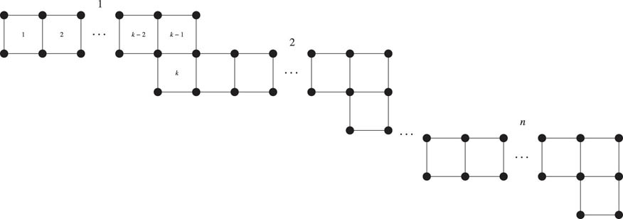
Specifically, polyomino systems, characterized by configurations of squares connected edge-to-edge, hold significant historical importance [23,24] and have found widespread applications across various scientific disciplines. In chemistry, their utility lies in their capacity to represent and analyze intricate chemical structures, including polymers, crystal structures, and specific organic molecules [25,26]. Notably, within this system, the polyomino chain stands out, where adjacent regular cells form a path by connecting their centers.

Within this framework, a square is classified as “terminal” if it has only one adjacent square, “medial” if it has two adjacent squares without any vertex of degree 2, and “kink” if it has two adjacent squares with a vertex of degree 2. A segment s is defined as a maximum linear chain along with a kink and/or terminal square. The count of squares within a segment is denoted by l ( S ) and indicates the length of the segment. By the way, a linear chain Li n comprises precisely one segment, while a zig-zag chain Z n consists of polyomino chains where all segments have lengths of 2 (Figure 1).

$Figure 1 The linear chain and the zigzag chain.$

Figure 1

The linear chain and the zigzag chain.

Transitioning to the random context, a random polyomino chain ( RPC n = RPC ( n , p ) ) can be generated as follows: Figure 2 illustrates RPC n for n = 1 and n = 2 . When n ≥ 3 , a new square can be added in two ways, leading to RPC n 1 and RPC n 2 with probabilities p and 1 − p , respectively (Figure 3), where 0 < p < 1 . Hence, a topological index of a random polyomino chain at time n becomes a random variable.

$Figure 2 The graphs of RPC 1 {{\rm{RPC}}}_{1} and RPC 2 {{\rm{RPC}}}_{2} .$

Figure 2

The graphs of RPC 1 and RPC 2 .

$Figure 3 The two link ways for RPC n ( n ≥ 3 ) {{\rm{RPC}}}_{n}\left(n\ge 3) .$

Figure 3

The two link ways for RPC n ( n ≥ 3 ) .

Continuing along the same vein, it is important to highlight that the calculation of different topological indices, extreme problems, and exploring topics, such as perfect pairings, dimer covering and their connection with caterpillar trees, among others [27–35], are active investigations on chains of polyominoes and chains of random polyominoes.

Inspired by the aforementioned research and our previous investigation of certain topological indices based on degree over random polyomino chains and polyomino chains [21], the primary objective of this manuscript is to establish explicit formulas for the first and second Zagreb connection indices. Additionally, we aim to analyze their extreme values within the context of polyomino chains. Under the random framework, our goal is to determine the expected values, variances, and asymptotic behavior.

This section aims to derive explicit mathematical expressions for computing the first Zagreb connection index and the second Zagreb connection index for a polyomino chain with n squares ( PC n ) denoted as ZC 1 , n and ZC 2 , n , respectively. Let m ≥ 1 and i ∈ { 1 , 2 , … , m } be given. It is worth noting that a polyomino chain PC n consists of a sequence of segments s 1 , s 2 , … , s m (refer to Figure 4) with lengths l ( s i ) = l i , satisfying the condition that ∑ i = 1 m l i = n + m − 1 . Moreover, a chain of polyominoes PC n induces a sequence of 1s and 2s as follows: If we denote L n as a random variable with rank { 1 , 2 } such that p = P ( L n = 1 ) , i.e., L n represents the selected link at time n , then we have a link of type j at time n if L n = j . By the way, here I A ( PC n ) ≔ I A takes the value of 1 if the statement described by A is true for PC n and zero otherwise. Having established this information, we proceed to present the two fundamental results of this section.

$Figure 4 Segments of a polyomino chain.$

Figure 4

Segments of a polyomino chain.

If PC n is a polyomino chain comprising n ≥ 4 squares and m ≥ 1 segment(s), then

ZC 1 , n = 2 ( 16 n + 10 m − 2 γ 1 + γ 2 + I { l 1 ≥ 4 } + I { l m ≥ 4 } − 34 ) ,

where γ 1 = ∑ i = 1 m I { l i = 2 } and γ 2 = ∑ i = 2 m − 2 I { l i = l i + 1 = 2 } .

Given PC n , conducting the one-step analysis

ZC 1 , n − ZC 1 , n − 1 = ∑ v ∈ V n , 1 τ n , v 2 + ∑ v ∈ V n , 2 ( τ n , v 2 − τ n − 1 , v 2 ) ,

where τ k , v ≔ τ v which is calculated within PC k , V n , 1 represents the vertices added when progressing from step n − 1 to n , and V n , 2 denotes the vertices that change their τ v during this advancement. By separately analyzing each sum, we obtain that

∑ v ∈ V n , 1 τ n , v 2 = 8 + 5 I { L n = 2 }

and

∑ v ∈ V n , 2 ( τ n , v 2 − τ n − 1 , v 2 ) = ∑ v ∈ V n , 2 ( ( τ n − 1 , v + 1 ) 2 − τ n − 1 , v 2 ) = ∣ V n , 2 ∣ + 2 ∑ v ∈ V n , 2 τ n − 1 , v = 4 + 2 ∑ i = 1 4 τ n − 1 , v i + ( 2 τ n − 1 , v 5 + 1 ) I { L n = 2 } ,

where the vertices v i for i ∈ { 1 , … , 5 } are located in the two end squares of the polyomino chain at time n − 1 , as shown in Figure 5. Substituting these values, we derive

ZC 1 , n = ZC 1 , n − 1 + 12 + 2 ( τ n − 1 , v 5 + 3 ) I { L n = 2 } + 2 ∑ i = 1 4 τ n − 1 , v i .

Now, we need to examine the values of τ n − 1 , v i for i ∈ { 1 , … , 5 } . They can be obtained using the above one-step analysis, but now considering the chain in reverse; since they form part of the two end squares of the polyomino chain at time n − 1 . Referring to this, Table 1 provides the corresponding values of τ n − 1 , v i in each entry, i.e., the entry in the nth row and ith column gives us the number of all the vertices in PC n − 1 situated at a distance of two from v i , where v i is one of the last six vertices of the PC n − 1 .

Therefore, for n ≥ 5

(2.1) ZC 1 , n = ZC 1 , n − 1 + g 1 ( L n − 2 , L n − 1 , L n ) ,

where

g 1 ( L n − 2 , L n − 1 , L n ) = 34 + 14 I { L n = 2 } − 2 I { L n − 2 = 1 , L n − 1 = L n = 2 } + 2 I { L n − 1 = 2 } − 2 I { L n − 2 = L n − 1 = 1 } .

From the information above, applying the recursive formula (2.1) for n ≥ 5 yields

(2.2) ZC 1 , n = ZC 1 , 4 + ∑ ( i , j , k ) ∈ { 1 , 2 } 3 g 1 ( i , j , k ) X i , j , k ,

where X i , j , k = ∣ { w ∈ { 5 , … , n } : L w − 2 = i , L w − 1 = j and L w = k in PC n } ∣ . Thus, upon substituting n = 4 into the preceding expression, we confirm the recovery of the initial value ZC 1 , 4 . Then, note that

X 1 , 1 , 1 + X 2 , 1 , 1 = X 1 , 1 − I { l 1 ≥ 4 } , X 1 , 1 , 2 + X 2 , 1 , 2 = X 1 , 2 − I { l 1 = 3 } , X 1 , 2 , 1 + X 2 , 2 , 1 = X 2 , 1 − I { l 1 = 2 , l 2 ≠ 2 } , X 1 , 2 , 2 + X 2 , 2 , 2 = X 2 , 2 − I { l 1 = l 2 = 2 } ,

where similarly X i , j = ∣ { w ∈ { 4 , … , n } : L w − 1 = i and L w = j in PC n } ∣ . Now, due to the values of g 1 and the above relations, equation (2.2) changes to

(2.3) ZC 1 , n = ZC 1 , 4 + 32 ( X 1 , 1 − I { l 1 ≥ 4 } ) + 46 ( X 1 , 2 − I { l 1 = 3 } ) + 36 ( X 2 , 1 − I { l 1 = 2 , l 2 ≠ 2 } ) + 48 ( X 2 , 2 − I { l 1 = l 2 = 2 } ) + 2 X 2 , 1 , 1 + 2 X 2 , 1 , 2 + 2 X 2 , 2 , 2 .

Attempting to condense the main expression once more, observe that

X 2 , 1 , 1 + X 2 , 1 , 2 = X 2 , 1 − I { l m = 3 } , X 1 , 1 + X 2 , 1 = X 1 − I { l 1 ≠ 2 } , X 2 , 2 + X 1 , 2 = X 2 − I { l 1 = 2 } , X 2 , 1 + X 2 , 2 = X 2 − I { l m = 2 } ,

where X 2 = ∣ { w ∈ { 3 , … , n } : L w = 2 in PC n } ∣ and X 1 = ∣ { w ∈ { 3 , … , n } : L w = 1 in PC n } ∣ . After this step, the updated equation (2.3) is

(2.4) ZC 1 , n = ZC 1 , 4 − 32 + 32 X 1 + 48 X 2 − 14 I { l 2 = 2 } − 2 I { l m = 2 } − 32 I { l 1 ≥ 4 } − 46 I { l 1 = 3 } − 36 I { l 1 = 2 , l 2 ≠ 2 } − 48 I { l 1 = l 2 = 2 } − 2 I { l m = 3 } + 4 X 2 , 1 + 2 X 2 , 2 , 2 .

Let us review the unknown variables: if at time w , L w = 2 , then the last segment in PC w − 1 is completed (initiating a new segment in PC w ). Conversely, if at time w , L w = 1 , then a square is added to the last segment in PC w − 1 . Hence, X 2 = m − 1 , X 1 = n − m − 1 , X 2 , 1 = m − γ 1 − 1 + I { l 1 = 2 } , and X 2 , 2 , 2 = γ 2 . To determine ZC 1 , 4 , we can use the same recursive expression, considering the values of τ 3 , v i . Thus,

ZC 1 , 4 = 84 + 12 I { L 4 = 2 } + 12 I { L 3 = 2 } = 84 + 12 I { l 1 = 3 } + 12 I { l 1 = 2 , l 2 ≠ 2 } + 24 I { l 1 = l 2 = 2 } .

Finally, substituting in (2.4) the values found and properly rewriting the excess terms, we obtain the result.□

$Figure 5 Vertices v i {v}_{i} in PC n − 1 {{\rm{PC}}}_{n-1} .$

Figure 5

Vertices v i in PC n − 1 .

Table 1

Values of τ n ‒ 1 , v i , where v i is one of the last six vertices of PC n ‒ 1

If PC n is a polyomino chain comprising n ≥ 5 squares and m ≥ 1 segment(s), then

ZC 2 , n = 48 n + 34 m − 9 γ 1 − 6 ∑ i = 1 , m I { l i = 2 } − 4 ∑ i = 1 , m I { l i = 3 } − 2 ∑ i = 1 , m I { l i = 4 } − ∑ i = 1 , m − 2 I { l i = l i + 1 = l i + 2 = 2 , m ≥ 3 } + I { l 1 = 2 , l 2 ≥ 4 , m ≥ 2 } + I { l m = 2 , l m − 1 ≥ 4 , m ≥ 2 } + γ 3 + γ 4 + γ 5 I { m ≥ 4 } − 112 ,

where γ 1 = ∑ i = 1 m I { l i = 2 } , γ 3 = ∑ i = 2 m − 2 I { l i + 1 = 3 ∨ l i = l i + 1 = 2 ∨ l i , l i + 1 ≠ 2 ∨ l i = 3 } , γ 4 = ∑ i = 1 m I { l i = 4 } , and γ 5 = 2 ∑ i = 3 m − 2 I { l i = 2 } − m + I { l 2 = 2 } + I { l m − 1 = 2 } + 3 .

By conducting the same analysis at one step, we conclude that

ZC 2 , n − ZC 2 , n − 1 = ∑ u v ∈ E n , 1 f n ( u v ) + ∑ u v ∈ E n , 2 ( f n ( u v ) − f n − 1 ( u v ) ) ,

where f k ( u v ) ≔ τ k , u τ k , v , E n , 1 are the edges that are added as we advance from step n − 1 to n and E n , 2 are the edges that modify their τ u τ v as we advance from step n − 1 to n . If we focus on each sum individually, it turns out that for n ≥ 6 ,

∑ u v ∈ E n , 1 f n ( u v ) = 16 + 2 I { L n − 1 = 2 , L n = 1 } + 8 I { L n = 2 }

and

∑ u v ∈ E n , 2 ( f n ( u v ) − f n − 1 ( u v ) ) = 4 + 2 ∑ i = 1 4 τ n − 1 , v i + ∑ i = 5 6 τ n − 1 , v i + ( τ n − 1 , v 4 + τ n − 1 , v 6 + 1 ) I { L n = 2 } + ( 4 − I { L n − 3 = 1 , L n − 2 = 2 } ) ( I { L n − 1 = 1 , L n = 2 } + I { L n − 1 = 2 } ) + I { L n − 1 = 2 } ,

where the vertices v i with i ∈ { 1 , … , 5 } are those used previously and the vertex v 6 is also presented in Figure 5. Then, substituting for n ≥ 6 , we obtain that

(2.5) ZC 2 , n = ZC 2 , n − 1 + g 2 ( L n − 3 , L n − 2 , L n − 1 , L n ) ,

where

g 2 ( L n − 3 , L n − 2 , L n − 1 , L n ) = 51 + 7 I { L n − 1 = 2 } + 17 I { L n = 2 } − I { L n − 2 = 1 , L n − 1 = 2 } − I { L n − 3 = L n − 2 = 1 } − 2 I { L n − 2 = L n − 1 = 1 } + 2 I { L n − 1 = 2 , L n = 1 } + 4 I { L n − 1 = 1 , L n = 2 } − I { L n − 3 = L n − 1 = 1 , L n − 2 = L n = 2 } − I { L n − 3 = 1 , L n − 2 = L n − 1 = 2 } − I { L n − 3 = L n − 2 = 1 , L n = 2 } .

Now, by applying the recursive formula (2.5) for n ≥ 6 , it follows that

(2.6) ZC 2 , n = ZC 2 , 5 + ∑ ( i , j , k , l ) ∈ { 1 , 2 } 4 g 1 ( i , j , k , l ) X i , j , k , l ,

where X i , j , k , l = ∣ { w ∈ { 6 , … , n } : L w − 3 = i , L w − 2 = j , L w − 3 = k , and L w = l in PC n } ∣ . Verifying that upon substituting n with 5 in the previous expression, we retrieve the initial value ZC 2 , 5 . Additionally,

X 1 , 1 , 1 , 1 + X 2 , 1 , 1 , 1 = X 1 , 1 , 1 − I { l 1 ≥ 5 } , X 1 , 1 , 1 , 2 + X 2 , 1 , 1 , 2 = X 1 , 1 , 2 − I { l 1 = 4 } , X 1 , 1 , 2 , 1 + X 2 , 1 , 2 , 1 = X 1 , 2 , 1 − I { l 1 = 3 , l 2 ≠ 2 } , X 1 , 1 , 2 , 2 + X 2 , 1 , 2 , 2 = X 1 , 2 , 2 − I { l 1 = 3 , l 2 = 2 } , X 1 , 2 , 1 , 1 + X 2 , 2 , 1 , 1 = X 2 , 1 , 1 − I { l 1 = 2 , l 2 ≥ 4 } , X 1 , 2 , 1 , 2 + X 2 , 2 , 1 , 2 = X 2 , 1 , 2 − I { l 1 = 2 , l 2 = 3 } , X 1 , 2 , 2 , 1 + X 2 , 2 , 2 , 1 = X 2 , 2 , 1 − I { l 1 = l 2 = 2 , l 3 ≠ 2 } , X 1 , 2 , 2 , 2 + X 2 , 2 , 2 , 2 = X 2 , 2 , 2 − I { l 1 = l 2 = l 3 = 2 } . X 2 , 1 , 1 , 1 + X 2 , 1 , 1 , 2 = X 2 , 1 , 1 − I { l m = 4 } , X 2 , 1 , 2 , 1 + X 2 , 1 , 2 , 2 = X 2 , 1 , 2 − I { l m − 1 = 3 , l m = 2 } , X 2 , 2 , 2 , 1 + X 2 , 2 , 2 , 2 = X 2 , 2 , 2 − I { l m − 2 = l m − 1 = l m − 2 = 2 } , X 2 , 2 , 1 + X 2 , 2 , 2 = X 2 , 2 − I { l m − 1 = l m = 2 } .

Therefore, using the above relations, together with the similar ones employed in Theorem 1 concerning X i , j , k and X i , j , it all boils down to expressing in terms of segment lengths X 2 , 1 , 1 , 2 , X 2 , 1 , 2 , 2 , X 2 , 2 , 1 , 2 , and ZC 2 , 5 . Finally, by performing some algebraic manipulations with the excess terms, the proof is complete.□

To complement the preceding theorems, Table 2 presents the values of the analyzed indices for the cases n ≤ 6 .

Table 2

Values of ZC 1 , n and ZC 2 , n for n ≤ 6

n	Links	ZC 1 ( PC n )	ZC 2 ( PC n )
2		24	28
3	1	52	68
	2	62	78
4	(1,1)	84	114
	(1,2) and (2,1)	96	131
	(2,2)	108	144
5	(1,1,1)	116	162
	(1,1,2) and (2,1,1)	130	181
	(1,2,1)	132	188
	(2,1,2)	144	200
	(1,2,2) and (2,2,1)	144	202
	(2,2,2)	158	216
6	(1,1,1,1)	148	210
	(1,1,1,2) and (2,1,1,1)	162	230
	(1,1,2,1) and (1,2,1,1)	166	239
	(2,1,1,2)	176	251
	(1,1,2,2) and (2,2,1,1)	178	253
	(1,2,1,2) and (2,1,2,1)	180	259
	(1,2,2,1)	180	261
	(2,1,2,2) and (2,2,1,2)	192	274
	(1,2,2,2) and (2,2,2,1)	194	276
	(2,2,2,2)	208	291

Now, we will utilize the main results to compute ZC 1 , n and ZC 2 , n for certain types of polyomino chains studied in the literature [25,36,37].

For the polyomino chain with n squares and two segments s 1 and s 2 satisfying that l 1 = 2 and l 2 = n − 1 , denoted as PC n 1 , we have the following:

ZC 1 , n = 32 n − 30 − 2 I { n = 4 } , n ≥ 4 , ZC 2 , n = 48 n − 58 − I { n = 5 } , n ≥ 5 .

For the polyomino chain with n squares and m ≥ 3 segments s 1 , s 2 , … , s m satisfying that l 1 = l m = 2 and l 2 , … , l m − 1 ≥ 3 , denoted as PC n 2 , we have the following:

ZC 1 , n = 32 n + 20 m − 76 , n ≥ 4 , ZC 2 , n = 48 n + 34 m − 140 − I { l 2 = 3 } − I { l m − 1 = 3 } + m 4 , n ≥ 5 ,

where m 4 denotes the number of segments of length equal to 4.

On the other hand, we denote a polyomino chain of dimension n ≥ 1 with k = k 1 + k 2 + k 3 , where k 1 is the number of kinks, k 2 is the number of medials, and k 3 is the number of terminals in a unit of polyomino chain, by PC n , k . Figure 6 illustrates a general representation of a polyomino chain PC n , k . Let k ≥ 3 , by definition of PC n , k , we have: m = 2 n , γ = n − 1 , I { l m = 2 } = 1 , and I { l 1 = 2 } = I { k = 3 } . Hence, in the following corollary, we will compute ZC 1 ( PC n , k ) and ZC 2 ( PC n , k ) for k ≥ 3 using Theorems 1 and 2.

$Figure 6 General representation of PC n , k {{\rm{PC}}}_{n,k} .$

Figure 6

General representation of PC n , k .

Note that by definition PC n , 1 = Li n and PC n , 2 = Z 2 n .

Given k ≥ 3 , n ≥ 2 , it follows that

ZC 1 ( PC n , k ) = n ( 32 k + 36 ) − 66 − 6 I { k = 3 } − 2 I { k = 4 } , ZC 2 ( PC n , k ) = n ( 48 k + 59 ) − 117 + ( 2 n − 19 ) I { k = 3 } + ( n − 5 ) I { k = 4 } − I { k = 5 } .

By definition, if PC n = Li n , we deduce that m = 1 and l 1 = n . Similarly, if PC n = Z n , then m = n − 1 and l i = 2 for i = 1 , 2 , … , m . Therefore, the following results can be obtained by applying the previous theorems.

Let Li n and Z n be linear and zigzag chains, respectively, with n ≥ 3 squares. Then

ZC 1 ( Li n ) ≤ ZC 1 ( PC n ) ≤ ZC 1 ( Z n ) .

Equality is attained if and only if PC n = Li n and PC n = Z n , respectively. Moreover, ZC 1 ( Li n ) = 32 n − 44 for n ≥ 3 and ZC 1 ( Z n ) = 50 n − 92 for n ≥ 4 .

The proof will proceed by induction on n . For n ≤ 6 , verification will be conducted based on Table 2. Now, assuming that the assertion holds for n − 1 , i.e.,

ZC 1 ( Li n − 1 ) ≤ ZC 1 , n − 1 ≤ ZC 1 ( Z n − 1 ) ,

and that equality is reached if and only if PC n − 1 = Li n − 1 , Z n − 1 , respectively. By utilizing the recursive formula provided in Theorem 1, for n ≥ 6 , we can assert that ZC 1 , n = ZC 1 , n − 1 + g 1 ( L n − 2 , L n − 1 , L n ) . Then, it can be verified that g 1 ( 1 , 1 , 1 ) = 32 ≤ g 1 ( L n − 2 , L n − 1 , L n ) ≤ 50 = g 1 ( 2 , 2 , 2 ) . Moreover, the equality holds if and only if L n − 2 = L n − 1 = L n = 1 and L n − 2 = L n − 1 = L n = 2 , respectively. Thus,

ZC 1 ( Li n − 1 ) + 32 = ZC 1 ( Li n ) ≤ ZC 1 , n ≤ ZC 1 ( Z n ) = ZC 1 ( Z n − 1 ) + 50 .

The proof is complete.□

Simply by working with g 2 ( L n − 3 , L n − 2 , L n − 1 , L n ) as it appears in the recursive formula presented in Theorem 2, a similar line of reasoning allows us to prove the following proposition.

Let Li n and Z n be linear and zigzag chains, respectively, with n ≥ 3 squares. Then

ZC 2 ( Li n ) ≤ ZC 2 ( PC n ) ≤ ZC 2 ( Z n ) .

Equality is achieved if and only if PC n = Li n and PC n = Z n , respectively. Moreover, ZC 2 ( Li n ) = 48 n − 78 for n ≥ 4 and ZC 2 ( Z n ) = 75 n − 159 for n ≥ 5 .

This remark aims to underscore certain implications of Theorems 1 and 2, which are derived similarly through the recursive formula and properties of the functions g 1 and g 2 .

Given that, for a fixed PC n , g 1 ( L n − 2 , L n − 1 , L n ) < g 2 ( L n − 3 , L n − 2 , L n − 1 , L n ) , it follows that for n ≥ 2 , ZC 1 , n < ZC 2 , n .
Because of the sequence of values of the function g 1 ( g 2 ) , substituting a link of type 1 with a link of type 2 in a fixed PC n leads to an increase in the index. After this, one might think that this property suggests that when the number of links equal to two ( X 2 ) increases then the index increases. However, this is generally not true, see the following examples written with the notation introduced in the following paragraph:
ZC i ( PC ( 2 , 2 , 2 , 1 , 1 , 1 , 1 , 1 , 1 , 2 , 2 ) ) < ZC i ( PC ( 1 , 1 , 2 , 1 , 2 , 1 , 2 , 1 , 2 , 1 , 1 ) ) , i = 1 , 2 , ZC 1 ( PC ( 1 , 2 , 1 , 2 , 1 , 2 , 1 , 2 , 1 , 1 ) ) = ZC 1 ( PC ( 2 , 2 , 1 , 1 , 1 , 1 , 1 , 2 , 2 , 2 ) ) ,
and
ZC 2 ( PC ( 1 , 2 , 1 , 1 , 1 , 2 , 1 , 1 , 1 , 1 , 1 , 1 ) ) = ZC 2 ( PC ( 2 , 2 , 1 , 1 , 1 , 1 , 1 , 1 , 1 , 1 , 1 , 2 ) ) .

The aforementioned propositions indicate where the maximum and minimum values are attained. Furthermore, Remark 2(b) allows us to compare certain types of chains. Similarly, the subsequent results provide insight into how the indices behave beyond the extremes. To facilitate the interpretation of the results, we will adopt the following notation: PC ( L 3 , L 4 , … , L n ) represents a polyomino chain with n squares, with the links chosen at each stage according to the vector v = ( L 3 , L 4 , … , L n ) . In the forthcoming two results, we will primarily focus on polyomino chains containing either one link of type 1 or one link of type 2 and the number of links preceding either the link of type 1 or the link of type 2 will be greater than or equal to ⌊ ( n − 2 ) ⁄ 2 ⌋ .

Given PC n with n ≥ 5 squares. Then

ZC 1 ( Li n ) < ZC 1 ( PC ( 1 , 1 , … , 1 , 2 ) ) < ZC 1 ( PC ( 1 , 1 , … , 1 , 2 , 1 ) ) < ZC 1 ( PC ( 1 , 1 , … , 1 , 2 , 1 , 1 ) ) = ZC 1 ( PC ( 1 , 1 , … , 1 ︸ i , 2 , 1 , … , 1 , 1 ) ) ,

and

ZC 1 ( Z n ) > ZC 1 ( PC ( 2 , 2 , … , 2 , 1 ) ) > ZC 1 ( PC ( 2 , 2 , … , 2 , 1 , 2 ) ) > ZC 1 ( PC ( 2 , 2 , … , 2 , 1 , 2 , 2 ) ) = ZC 1 ( PC ( 2 , 2 , … , 2 ︸ i , 1 , 2 , … , 2 , 2 ) ) ,

with ⌊ ( n − 2 ) ⁄ 2 ⌋ ≤ i ≤ n − 6 . Moreover, for n ≥ 6

ZC 1 ( PC ( 1 , 1 , … , 1 , 2 , 1 , 1 ) ) < ZC 1 ( PC ( 2 , 1 , … , 1 , 2 ) )

and

ZC 1 ( PC ( 2 , 2 , … , 2 , 1 , 2 , 2 ) ) > ZC 1 ( PC ( 1 , 2 , … , 2 , 1 ) ) .

Note that, for n = 5 , 6 , the result is verified according to Table 2. Therefore, we will prove it for n ≥ 7 . The first inequality follows from Proposition 3 (also by Remark 2 (b)). For the second inequality, observe that, by symmetry, PC ( 1 , 1 , … , 1 , 2 ) = PC ( 2 , 1 , … , 1 , 1 ) . Thus, by applying the recursive formula presented in Theorem 1, we conclude that

ZC 1 ( PC ( 2 , 1 , … , 1 , 1 ︸ n − 3 ) ) = ZC 1 ( PC ( 2 , 1 , … , 1 ︸ n − 4 ) ) + g 1 ( 1 , 1 , 1 )

and

ZC 1 ( PC ( 1 , 1 , … , 1 , 2 , 1 ) ) = ZC 1 ( PC ( 1 , 1 , … , 1 , 2 ) ) + g 1 ( 1 , 2 , 1 ) .

Given that the first summands are equal by symmetry and g 1 ( 1 , 1 , 1 ) < g 1 ( 1 , 2 , 1 ) , the required result follows. The third inequality can be verified through a similar analysis, thus, we will proceed to prove the final part. To do this, we will demonstrate that:

ZC 1 ( PC ( 1 , 1 , … , 1 ︸ i , 2 , 1 , … , 1 , 1 ) ) = ZC 1 ( PC ( 1 , 1 , … , 1 ︸ i − 1 , 2 , 1 , … , 1 , 1 ) ) ,

with ⌊ ( n − 2 ) ⁄ 2 ⌋ + 1 ≤ i ≤ n − 5 . In this case, rewriting the expressions as follows:

ZC 1 ( PC ( 1 , 1 , … , 1 ︸ i , 2 , 1 , … , 1 , 1 ) ) = ZC 1 ( PC ( 1 , 1 , … , 1 , 2 , 1 , … , 1 , 1 ︸ i − 1 ) ) + g 1 ( 1 , 1 , 1 )

and

ZC 1 ( PC ( 1 , 1 , … , 1 ︸ i − 1 , 2 , 1 , … , 1 , 1 ) ) = ZC 1 ( PC ( 1 , 1 , … , 1 ︸ i − 1 , 2 , 1 , … , 1 , 1 ) ) + g 1 ( 1 , 1 , 1 ) ,

since i ≥ 3 and n − 2 − i ≥ 3 , we conclude the equalities. For the decreasing inequalities, we proceed similarly,

considering that g 1 ( 2 , 2 , 2 ) is the maximum. As for the final inequalities, which involve a chain with two links of type 2 and two links of type 1, respectively, by iterating the recursive formula, it is demonstrated that

ZC 1 ( PC ( 2 , 1 , … , 1 , 2 ) ) − ZC 1 ( PC ( 1 , 1 , … , 1 , 2 , 1 , 1 ) ) = g 1 ( 1 , 1 , 1 ) + g 1 ( 1 , 1 , 2 ) − g 1 ( 1 , 2 , 1 ) − g 1 ( 2 , 1 , 1 )

and

ZC 1 ( PC ( 1 , 2 , … , 2 , 1 ) ) − ZC 1 ( PC ( 2 , 2 , … , 2 , 1 , 2 , 2 ) ) = g 1 ( 2 , 2 , 2 ) + g 1 ( 2 , 2 , 1 ) − g 1 ( 2 , 1 , 2 ) − g 1 ( 1 , 2 , 2 ) .

Now, since g 1 ( 1 , 1 , 1 ) + g 1 ( 1 , 1 , 2 ) − g 1 ( 1 , 2 , 1 ) − g 1 ( 2 , 1 , 1 ) > 0 and g 1 ( 2 , 2 , 2 ) + g 1 ( 2 , 2 , 1 ) − g 1 ( 2 , 1 , 2 ) − g 1 ( 1 , 2 , 2 ) < 0 , the proof is complete.□

Using a similar approach, we obtain the following proposition.

Given PC n with n ≥ 5 squares. Then

ZC 2 ( Li n ) < ZC 2 ( PC ( 1 , 1 , … , 1 , 2 ) ) < ZC 2 ( PC ( 1 , 1 , … , 1 , 2 , 1 ) ) < ZC 2 ( PC ( 1 , 1 , … , 1 , 2 , 1 , 1 ) ) < ZC 2 ( PC ( 1 , 1 , … , 1 , 2 , 1 , 1 , 1 ) ) = ZC 2 ( PC ( 1 , 1 , … , 1 ︸ i , 2 , 1 , … , 1 , 1 ) )

and

ZC 2 ( Z n ) > ZC 2 ( PC ( 2 , 2 , … , 2 , 1 ) ) > ZC 2 ( PC ( 2 , 2 , … , 2 , 1 , 2 ) ) > ZC 2 ( PC ( 2 , 2 , … , 2 , 1 , 2 , 2 ) ) > ZC 2 ( PC ( 2 , 2 , … , 2 , 1 , 2 , 2 ) ) = ZC 2 ( PC ( 2 , 2 , … , 2 ︸ i , 1 , 2 , … , 2 , 2 ) ) ,

with ⌊ ( n − 2 ) ⁄ 2 ⌋ ≤ i ≤ n − 7 . Moreover, for n ≥ 8

ZC 2 ( PC ( 1 , 1 , … , 1 , 2 , 1 , 1 , 1 ) ) < ZC 2 ( PC ( 2 , 1 , … , 1 , 2 ) ) ,

and

ZC 2 ( PC ( 2 , 2 , … , 2 , 1 , 2 , 2 , 2 ) ) > ZC 2 ( PC ( 1 , 2 , … , 2 , 1 ) ) .

Similarly, it is possible to show that, for n ≥ 6 and i = 1 , 2

ZC i ( PC ( 1 , 2 , … , 2 , 1 ) ) > ZC i ( PC ( 2 , 1 , … , 1 , 2 ) ) .

Hence, combining this with the results detailed in the previous propositions, the ascending and descending sequences in both indices can be connected for n ≥ 5 . On the other hand, when comparing Proposition 5 with Proposition 6, it is noted that the latter includes an additional inequality. This is primarily attributed to the fact that the function g 2 involves four variables, whereas the function g 1 comprises three. In fact, as per the findings presented in [21], the recursive formula for the degree-based topological indices on the PC n is governed by a function of two variables. Consequently, the question arises as to when similar behaviors persist and when distinct patterns emerge for different degree-based topological indices. Finally, it is crucial to note, although it is not explicitly stated in the above propositions, that due to symmetry

PC ( 1 , 1 , … , 1 ︸ i , 2 , 1 , … , 1 , 1 ︸ n − i − 3 ) = PC ( 1 , 1 , … , 1 ︸ n − i − 3 , 2 , 1 , … , 1 , 1 ︸ i )

and

PC ( 2 , 2 , … , 2 ︸ i , 1 , 2 , … , 2 , 2 ︸ n − i − 3 ) = PC ( 2 , 2 , … , 2 ︸ n − i − 3 , 1 , 2 , … , 2 , 2 ︸ i ) .

This was the reason why the prepositions were raised only for i ≥ ⌊ ( n − 2 ) ⁄ 2 ⌋ .

To close this section we would like to highlight the following. Inspired by the above results other questions naturally arise: What happens to the behavior of the indices when the number of links of type 2 is not only 1 and n − 1 (similarly for the number of links of type 1), and Can we identify any patterns? Given n and X 2 fixed or equivalently given n and m fixed, it can be shown by focusing on the non-fixed summands of the expressions obtained in Theorems 1 and 2 the following: The minimum value of ZC i with i = 1 , 2 is

ZC i ( PC ( 2 , … , 2 ︸ ⌊ X 2 ⁄ 2 ⌋ , 1 , … , 1 , 2 , … , 2 ︸ ⌈ X 2 ⁄ 2 ⌉ ) ) .

In turn, the maximum value of ZC 1 is

ZC 1 ( PC ( 1 , … , 1 , ︸ 2 + ⌊ n − 2 X 2 − 5 2 ⌋ 2 , 1 , … , 2 , 1 ︸ 2 X 2 , 1 , … , 1 ︸ 1 + ⌈ n − 2 X 2 − 5 2 ⌉ ) ) ,

if ( n − 5 ) ⁄ 2 ≥ X 2 and the maximum value of ZC 2 is

ZC 2 ( PC ( 1 , 1 , … , 1 , ︸ 3 + ⌊ n − 3 X 2 − 6 2 ⌋ 2 , 1 , 1 , … , 2 , 1 , 1 ︸ 3 X 2 , 1 , … , 1 , 1 ︸ 1 + ⌈ n − 3 X 2 − 6 2 ⌉ ) ) ,

if ( n − 6 ) ⁄ 3 ≥ X 2 . Another relevant question would be to examine the possible patterns that arise when analyzing the behavior between the minimum and maximum values of all polyomino chains while keeping the values of n and X 2 fixed. We intend to explore this in future work.

In this section, we introduce and demonstrate our main results within a randomized framework, offering insights into long-term behavior. We will employ the symbols ⟶ a . s and ⟶ D to denote convergence in almost surely and distribution, respectively. Here, N ( μ , σ 2 ) represents a random variable following a normal distribution with mean μ and variance σ 2 , and Mult ( n , p ) represents a random variable following a multinomial distribution with parameters n and p .

As n → ∞ ,

ZC 1 , n − ( 50 − 18 p + 2 p 2 − 2 p 3 ) n n ⟶ D N ( 0 , σ 2 ) ,

where σ 2 = 4 p ( 1 − p ) ( 5 p 4 − 7 p 3 + 56 p 2 − 35 p + 81 ) .

Based on the recursive relation found in Theorem 1, we can express ZC 1 , n for n ≥ 4 as follows:

ZC 1 , n = ZC 1 , 4 + ∑ i = 3 n − 2 G 1 ( Y i ) ,

where Y i = L i L i + 1 L i + 2 , i.e., it is the random variable that gives me how the last three links used up to the time i + 2 have been appearing and G 1 ( a b c ) ≔ g 1 ( a , b , c ) for a b c ∈ S ≔ { 111 , 112 , … , 221 , 222 } . According to the definition, we have that { Y i } i ≥ 3 corresponds to a homogeneous Markov Chain with transition probability as follows:

P ( Y 4 = d e f ∣ Y 3 = a b c ) = p 2 − f ( 1 − p ) f − 1 if b = d , c = e 0 otherwise ,

with a b c , d e f ∈ S . As a first consequence of the probability of transition we have that: any pair of states can be linked within three steps with a positive probability, since

P ( Y 6 = d e f ∣ Y 3 = a b c ) = P ( Y 4 = b c d ∣ Y 3 = a b c ) P ( Y 5 = c d e ∣ Y 4 = b c d ) P ( Y 6 = d e f ∣ Y 5 = c d e ) = p 6 − ( d + e + f ) ( 1 − p ) ( d + e + f ) − 3 > 0 .

Thus, each entry of P 3 is positive, where P denotes the transition matrix of the homogeneous Markov Chain { Y i } i ≥ 3 . In this way, the properties of irreducibility and aperiodicity are proved simultaneously. At this point based on the Perron-Frobenius theorem [38,39], we have that the limit distribution exists. On the other hand, the initial distribution π 3 verifies that

π 3 ( d e f ) = P ( Y 3 = d e f ) = p 6 − ( d + e + f ) ( 1 − p ) ( d + e + f ) − 3 .

With this clarification, we can see that another implication of the transition probability is that the initial distribution π 3 is the limiting distribution, because

∑ a b c ∈ S π 3 ( a b c ) P ( Y 4 = d e f ∣ Y 3 = a b c ) = p 2 − f ( 1 − p ) f − 1 ∑ a ∈ { 1 , 2 } π 3 ( a d e ) = p 6 − ( d + e + f ) ( 1 − p ) ( d + e + f ) − 3 = π 3 ( d e f ) .

Now, considering the measurable real-valued function G 1 for which V π 3 ( G 1 ( Y 3 ) ) < + ∞ , by virtue of the Markov chain central limit theorem [40,41 ], we deduce that

ZC 1 , n − E π 3 ( G 1 ( Y 3 ) ) n n ⟶ D N ( 0 , σ G 1 2 ) ,

where σ G 1 2 = V π 3 ( G 1 ( Y 3 ) ) + 2 C o v π 3 ( G 1 ( Y 3 ) , G 1 ( Y 4 ) ) + 2 C o v π 3 ( G 1 ( Y 3 ) , G 1 ( Y 5 ) ) , as Y 3 is independent of Y k for k ≥ 6 . Finally, making the required computations, the proof is complete.□

Conforming to the proof of Theorem 7, the probability of transition in three steps just depends on the final state, and furthermore, the rows of P 3 are the initial distribution π 3 . Using the result found for P 3 , we can similarly express each entry of P 4 as follows:

P ( Y 7 = d e f ∣ Y 3 = a b c ) = ∑ i ∈ { 1 , 2 } p 2 − i ( 1 − p ) i − 1 π 3 [ d e f ] = π 3 [ d e f ] .

Hence, P 3 = P 4 and as a consequence P n = P 3 , for n ≥ 3 . It is noteworthy to emphasize that the aforementioned procedure provides an alternative method to demonstrate that the stationary distribution of the Markov Chain is the initial distribution. By the way, the fact that the initial distribution is the stationary distribution indicates that the variables Y i are identically distributed, which means that they are independent of n . Specifically, Y i ∼ y ˆ ⋅ Mult ( 1 , p ˆ ) and G 1 ( Y i ) ∼ g ˆ 1 ⋅ Mult ( 1 , p ˆ ) with y ˆ = ( 1 1 1 , 1 1 2 , … , 2 2 1 , 2 2 2 ) , g ˆ 1 = ( g 1 ( 1 , 1 , 1 ) , g 1 ( 1 , 1 , 2 ) , … , g 1 ( 2 , 2 , 1 ) , g 1 ( 2 , 2 , 2 ) ) and p ˆ = ( p 3 , p 3 ( 1 − p ) , … , p ( 1 − p ) 2 , ( 1 − p ) 3 ) .

The proof of the following theorem uses a similar approach as the proof of the previous theorem.

As n → ∞ ,

ZC 2 , n − ( 75 − 23 p + 4 p 2 − 13 p 3 + 5 p 4 ) n n ⟶ D N ( 0 , σ 2 ) ,

where σ 2 = 11,250 − 6,796 p + 2176 p 2 − 3,690 p 3 + 1,820 p 4 − 152 p 5 .

To complement the results found in Theorems 7 and 8, let us consider the following propositions.

Given a random polyomino chain with n squares, it follows that

E ( ZC 1 , n ) = 50 n − 92 − 6 ( 3 n − 8 ) p + 2 ( n − 4 ) p 2 ( 1 − p ) ,

for n ≥ 4 and

V ( ZC 1 , n ) = 4 ( − 6,972 + ( 324 n + 2,680 ) p + ( − 464 n + 1,360 ) p 2 + ( 364 n − 1,584 ) p 3 + ( − 252 n + 1,128 ) p 4 + ( 48 n − 256 ) p 5 + ( − 20 n + 104 ) p 6 ) ,

for n ≥ 6 . Moreover, ZC 1 , n is asymptotically concentrated around its mean. More precisely, as n → ∞ , ZC 1 , n n ⟶ a . s 50 − 18 p + 2 p 2 − 2 p 3 .

Note that the expression for the expectation follows directly from the recursive relation studied in the preceding section. With this initial result in hand, we can derive the expression for the variance by calculating the second moment and applying the recursive relation as follows:

ZC 1 , n 2 = ZC 1 , n − 1 2 + 2 ZC 1 , n − 1 g 1 ( L n − 2 , L n − 1 , L n ) + g 1 2 ( L n − 2 , L n − 1 , L n )

and

ZC 1 , n − 1 = Z C 1 n − 3 + g 1 ( L n − 4 , L n − 3 , L n − 2 ) + g 1 ( L n − 3 , L n − 1 , L n − 1 ) ,

with ZC 1 , n − 3 independent of g 1 ( L n − 2 , L n − 1 , L n ) . The second part is obtained by using the Strong Law of Large Numbers for Markov Chains [40, 41].□

Given a random polyomino chain with n squares, it follows that

E ( ZC 2 , n ) = 75 n − 159 + ( − 23 n + 71 ) p + ( 4 n − 30 ) p 2 + ( − 134 n + 65 ) p 3 + 5 ( n − 5 ) p 4 ,

for n ≥ 5 and

V ( ZC 2 , n ) = 33,750 n − 1,15,200 + ( − 19,893 n + 91,222 ) p + ( 5,279 n − 93,671 ) p 2 + ( − 8,799 n + 127,136 ) p 3 + ( 2,593 n − 48,519 ) p 4 + ( 1,930 n − 11,394 ) p 5 + ( − 1,751 n + 12,579 ) p 6 + ( 890 n − 5,954 ) p 7 + ( − 175 n + 1,177 ) p 8 ,

for n ≥ 8 . Moreover, ZC 2 , n is asymptotically concentrated around its mean. More precisely, as n → ∞ , ZC 2 , n n ⟶ a . s 75 − 23 p + 4 p 2 − 13 p 3 + 5 p 4 .

The demonstration proceeds similarly, with the only variation being that in this particular case,

ZC 2 , n − 1 = ZC 2 , n − 4 + g 2 ( L n − 6 , L n − 5 , L n − 4 , L n − 3 ) + g 2 ( L n − 5 , L n − 4 , L n − 3 , L n − 2 ) + g 2 ( L n − 4 , L n − 3 , L n − 2 , L n − 1 )

with ZC 2 , n − 4 independent of g 2 ( L n − 3 , L n − 2 , L n − 1 , L n ) . The second part is performed as before.□

As mentioned above, a recursive formula for degree-based topological indices over PC n was derived in [21] and the asymptotic behavior and other characteristics for certain types of degree-based topological indices over RPC n , such as the generalized Zagreb index, were also studied. Again, we have a recursive formula; only in this case, it is governed by a function of two variables. Thus, the same procedure (with slight differences) performed for ZC 1 , n and ZC 2 , n works, giving us information about the expected value, variance, and asymptotic behavior of any degree-based topological index over RPC n (obviously encompassing those already covered in [21]).

In this study, we have investigated the first and second Zagreb connection indices of polyomino chains and random polyomino chains using a Markov chain approach. Specifically, we have computed these indices within polyomino chains, explored extreme graphs, and outlined several patterns. In addition, we have formulated a central limit theorem concerning random polyomino chains. Finally, it would be interesting to extend the work of this article to k -polygonal chains or other types of topological indices following the same methodology.

The authors are deeply grateful to the reviewers and the Associate Editor for their careful reading of the original manuscript and for their advice to improve the article.

Funding information: This work was partially supported by VIEP under Grant No. 00389.
Author contributions: All authors have accepted responsibility for the entire content of this manuscript and consented to its submission to the journal, reviewed all the results, and approved the final version of the manuscript. SS and HCS obtained the main results. SS prepared the manuscript with the contributions of HCS.
Conflict of interest: The authors do not declare a conflict of interest.

[1] H. Wiener, Structural determination of paraffin boiling points, J. Am. Chem. Soc. 69 (1947), no. 1, 17–20. 10.1021/ja01193a005Search in Google Scholar PubMed

[2] V. R. Kulli, Graph indices, Handbook of Research on Advanced Applications of Graph Theory in Modern Society, IGI Global, Hershey, Pennsylvania, USA, 2020, pp. 66–91. 10.4018/978-1-5225-9380-5.ch003Search in Google Scholar

[3] A. Rauf, M. Naeem, and S. U. Bukhari, Quantitative structure-property relationship of Ev-degree and Ve-degree based topological indices: physico-chemical properties of benzene derivatives, Int. J. Quantum Chem. 122 (2021), no. 5, e26851. 10.1002/qua.26851Search in Google Scholar

[4] Z. Shao, A. Jahanbani, and S. M. Sheikholeslami, Multiplicative topological indices of molecular structure in anticancer drugs, Polycycl. Aromat. Comp. 42 (2020), no. 2, 475–488. 10.1080/10406638.2020.1743329Search in Google Scholar

[5] I. Gutman and N. Trinajstić, Graph theory and molecular orbitals. Total varphi-electron energy of alternant hydrocarbons, Chem. Phys. Lett. 17 (1972), no. 4, 535–538. 10.1016/0009-2614(72)85099-1Search in Google Scholar

[6] I. Gutman, B. Ruščič, N. Trinajstić, and C. F. Wilcox, Graph theory and molecular orbitals. XII. Acyclic polyenes, J. Chem. Phys. 62 (1975), no. 9, 3399–3405. 10.1063/1.430994Search in Google Scholar

[7] I. Gutman, A. M. Naji, and N. D. Soner, On leap Zagreb indices of graphs, Commun. Comb. Optim. 2 (2017), no. 2, 99–117. Search in Google Scholar

[8] A. Ali and N. Trinajstić, A novel/old modification of the first Zagreb index, Mol. Inform. 37 (2018), no. 6–7, 1800008. 10.1002/minf.201800008Search in Google Scholar PubMed

[9] A. Ullah, S. Zaman, and A. Hamraz, Zagreb connection topological descriptors and structural property of the triangular chain structures, Phys. Scr. 98 (2023), no. 2, 025009. 10.1088/1402-4896/acb327Search in Google Scholar

[10] D. Balasubramaniyan, N. Chidambaram, V. Ravi, and M. K. Siddiqui, Qspr analysis of anti-asthmatic drugs using some new distance-based topological indices: A comparative study, Int. J. Quantum Chem. 124 (2024), no. 9, e27372. 10.1002/qua.27372Search in Google Scholar

[11] Z. Raza and M. Imran, Expected values of some molecular descriptors in random cyclooctane chains, Symmetry 13 (2021), no. 11, 2197.10.3390/sym13112197Search in Google Scholar

[12] S. Wei, X. Ke, and Y. Wang, Wiener indices in random cyclooctane chains, Wuhan Univ. J. Nat. Sci. 23 (2018), no. 6, 498–502. 10.1007/s11859-018-1355-5Search in Google Scholar

[13] Z. Raza, K. Naz, and S. Ahmad, Expected values of molecular descriptors in random polyphenyl chains, Emerg. Sci. J. 6 (2022), no. 1, 151–165. 10.28991/ESJ-2022-06-01-012Search in Google Scholar

[14] X. Ke, S. Wei, and J. Huang, The atom-bond connectivity and geometric-arithmetic indices in random polyphenyl chains, Polycycl. Aromat. Comp. 41 (2021), no. 9, 1873–1882. 10.1080/10406638.2019.1703763Search in Google Scholar

[15] Z. Raza, The expected values of arithmetic bond connectivity and geometric indices in random phenylene chains, Heliyon 6 (2020), no. 7. 10.1016/j.heliyon.2020.e04479Search in Google Scholar PubMed PubMed Central

[16] Z. Raza, The expected values of some indices in random phenylene chains, Eur. Phys. J. Plus 136 (2021), no. 1, 1–15. 10.1140/epjp/s13360-021-01082-ySearch in Google Scholar

[17] A. Jahanbani, The first Zagreb and Randić indices in random spiro chains, Polycycl. Aromat. Comp. 42 (2020), no. 4, 1842–1850. 10.1080/10406638.2020.1809471Search in Google Scholar

[18] S. Sigarreta, S. Sigarreta, and H. Cruz-Suárez, On bond incident degree indices of random spiro chains, Polycycl. Aromat. Comp. 43 (2023), no. 7, 6306–6318. 10.1080/10406638.2022.2118795Search in Google Scholar

[19] A. A. Dobrynin, I. Gutman, S. Klavžar, and P. Žigert, Wiener index of hexagonal systems, Acta Appl. Math. 72 (2002), 247–294. 10.1023/A:1016290123303Search in Google Scholar

[20] J. B. Liu, Y. Q. Zheng, and X. B. Peng, The statistical analysis for sombor indices in a random polygonal chain networks, Discrete Appl. Math. 338 (2023), 218–233. 10.1016/j.dam.2023.06.006Search in Google Scholar

[21] S. Sigarreta, S. Sigarreta, and H. Cruz-Suárez, On degree-based topological indices of random polyomino chains, Math. Biosci. Eng. 19 (2022), no. 9, 8760–8773. 10.3934/mbe.2022406Search in Google Scholar PubMed

[22] Z. Raza, S. Akhter, and Y. Shang, Expected value of first Zagreb connection index in random cyclooctatetraene chain, random polyphenyls chain, and random chain network, Front. Chem. 10 (2023), 1067874. 10.3389/fchem.2022.1067874Search in Google Scholar PubMed PubMed Central

[23] S. W. Golomb, Checker boards and polyominoes, Amer. Math. Monthly 61 (1954), no. 10, 675–682. 10.1080/00029890.1954.11988548Search in Google Scholar

[24] S. W. Golomb, Polyominoes: Puzzles, Patterns, Problems, and Packings, Princeton University Press, Princeton, New Jersey, USA, 1994. 10.1515/9780691215051Search in Google Scholar

[25] A. Farooq, M. Habib, A. Mahboob, W. Nazeer, and S. M. Kang, Zagreb polynomials and redefined Zagreb indices of dendrimers and polyomino chains, Open Chem. 17 (2019), no. 1, 1374–1381. 10.1515/chem-2019-0144Search in Google Scholar

[26] W. Gao, L. Yan, and L. Shi, Generalized Zagreb index of polyomino chains and nanotubes, Optoelectron. Adv. Mat. 11 (2017), 119–124. Search in Google Scholar

[27] J. Rada, The linear chain as an extremal value of VDB topological indices of polyomino chains, Appl. Math. Sci. 8 (2014), 5133–5143. 10.12988/ams.2014.46507Search in Google Scholar

[28] J. Rada, The zig-zag chain as an extremal value of VDB topological indices of polyomino chains, J. Combin. Math. Combin. Comput. 96 (2016), 103–111. Search in Google Scholar

[29] A. Ali, Z. Raza, and A. A. Bhatti, Bond incident degree (bid) indices of polyomino chains: a unified approach, Appl. Math. Comput. 287 (2016), 28–37. 10.1016/j.amc.2016.04.012Search in Google Scholar

[30] S. Li and W. Yan, Kekulé structures of polyomino chains and the Hosoya index of caterpillar trees, Discrete Math. 312 (2012), no. 15, 2397–2400. 10.1016/j.disc.2012.03.041Search in Google Scholar

[31] T. Wu, H. Lu, and X. Zhang, Extremal matching energy of random polyomino chains, Entropy 19 (2017), no. 12, 684. 10.3390/e19120684Search in Google Scholar

[32] S. Wei and W. C. Shiu, Enumeration of Wiener indices in random polygonal chains, J. Math. Anal. Appl. 469 (2019), no. 2, 537–548. 10.1016/j.jmaa.2018.09.027Search in Google Scholar

[33] S. Wei, X. Ke, and F. Lin, Perfect matchings in random polyomino chain graphs, J. Math. Chem. 54 (2016), no. 3, 690–697. 10.1007/s10910-015-0580-9Search in Google Scholar

[34] J. Li and W. Wang, The (degree-) Kirchhoff indices in random polygonal chains, Discrete Appl. Math. 304 (2021), 63–75. 10.1016/j.dam.2021.06.020Search in Google Scholar

[35] C. Xiao and H. Chen, Dimer coverings on random polyomino chains, Z. Naturforsch. A 70 (2015), no. 6, 465–470. 10.1515/zna-2015-0121Search in Google Scholar

[36] Y. C. Kwun, A. Farooq, W. Nazeer, Z. Zahid, S. Noreen, and S. M. Kang, Computations of the M-polynomials and degree-based topological indices for dendrimers and polyomino chains, Int. J. Anal. Chem. 2018 (2018), no. 1, 1709073. 10.1155/2018/1709073Search in Google Scholar PubMed PubMed Central

[37] S. Hayat, S. Ahmad, H. M. Umair, and S. Wang, Distance property of chemical graphs, Hacet. J. Math. Stat. 47 (2018), no. 5, 1071–1093. 10.15672/HJMS.2017.487Search in Google Scholar

[38] Y. Kifer, Perron-frobenius theorem, large deviations, and random perturbations in random environments, Math. Z. 222 (1996), 677–698. 10.1007/PL00004551Search in Google Scholar

[39] E. Seneta, Non-negative Matrices and Markov Chains, Springer Science & Business Media, New York, USA, 2006. Search in Google Scholar

[40] M. Rosenblatt, The central limit theorem for stationary processes, Proceedings of the Sixth Berkeley Symposium on Mathematical Statistics and Probability; 1972. Search in Google Scholar

[41] S. Brooks, A. Gelman, G. Jones, and X. L. Meng, Handbook of Markov Chain Monte Carlo, CRC Press, Boca Raton, Florida, USA, 2011. 10.1201/b10905Search in Google Scholar

Received: 2024-05-20

Revised: 2024-08-05

Accepted: 2024-08-06

Published Online: 2024-09-21

This work is licensed under the Creative Commons Attribution 4.0 International License.

2 + I { L 3 = 2 }

4 ‒ I { L 3 = L 4 = 1 }

2 + I { L 4 = 2 }

4 ‒ I { L 3 = 1 , L 4 = 2 }

4 ‒ I { L n ‒ 2 = L n ‒ 1 = 1 }

2 + I { L n ‒ 1 = 2 }

4 ‒ I { L n ‒ 2 = 1 , L n ‒ 1 = 2 }

5 ‒ I { L n ‒ 3 = L n ‒ 2 = 1 }

https://doi.org/10.1515/math-2024-0057

Keywords for this article

mathematical chemistry; topological indices; Markov chain; random graphs; polyomino chains

Creative Commons

BY 4.0