Long-term viscoelastic behavior and evolution of the Schapery model for mirror epoxy

1 Introduction

Epoxy resins are thermosetting resins [1,2,3]. Since their discovery in 1909 by Prileschajew [4], they have been increasingly interesting owing to some excellent mechanical properties, especially good resistance to chemicals and high adhesiveness to many substrates [5,6,7,8,9,10,11,12]. Epoxy resins are extensively used in paint and coating, industrial tooling, the aerospace industry, electronic equipment, and biomedical systems [13].

The field of civil engineering and flooring is experiencing great progress in the use of resins because they are robust, seamless, easy to maintain, and dustproof [14]. “3D epoxy” technology is the most recent in the development of mirror resins, which is characterized by its ease of cleaning, waterproofness, transparency, and indoor and outdoor application. It can be placed in any room of the house with a wide choice of pictures, which allows us to create an atmosphere and an effect of surprise even in small spaces. Mirror epoxy resins are bicomponent materials obtained by the polymerization of an epoxy monomer and a hardener. The resin/hardener ratio varies depending on the type of the resin, the hardener, and the field of application [15]. It directly influences the properties and mechanical characteristics of the material [16]. Each application has specific requirements in terms of mechanical properties, chemical resistance, durability, transparency, etc. These must be taken into account when choosing the appropriate resin and hardener.

There is a great concern with the study of epoxy and its mechanical behavior, with and without reinforcement. A new resin/hardener ratio, new types of resins, and hardeners or new improvement additives are emerging with each new study.

Mirror resins are bicomponent materials used in their pure state with a resin/hardener ratio of 100:50. They have a nonlinear viscoelastic behavior. Their mechanical properties vary over time and depend on the applied load. Therefore, the law of superposition is not valid here. For these materials, modeling is often done by introducing nonlinearity factors into Boltzmann’s law. One of the first models based on this method is that of Leaderman [17], which introduces a nonlinearity function in the integral. Other models that take this approach were presented by Bernstein et al. [18] and Green and Rivlin [19]. The most widely used model to describe nonlinear viscoelasticity is that of Schapery [20,21,22]. It is often used to predict the long-term behavior of materials, such as relaxation and creep, which are important phenomena in many industrial applications. To move into the nonlinear domain, Schapery used the principles of the thermodynamics of irreversible processes. In this model, Boltzman’s superposition principle is modified by introducing nonlinear functions.

Gmir et al. [23] have successfully used the law of Schapery to characterize the nonlinear viscoelastic behavior creep type of PMMA. The nonlinearity coefficients were determined by creep tests at 23°C, followed by an iterative program based on the rule of least squares.

In the present work, the same resolution method under the same test conditions was used to identify the nonlinear viscoelastic constitutive law of pure mirror resin at a resin/hardener ratio of 100:50 and at 23°C.

This study delves into the evolution of the Schapery model within the realm of long-term viscoelastic materials, with a specific focus on mirror epoxy in 3D flooring, an emerging innovation in building materials. It enhances our comprehension of the viscoelastic properties of this novel material, shedding light on its durability and stability over time. By intricately analyzing creep and relaxation mechanisms, this research surpasses mere initial characterization. Furthermore, it contributes to the advancement of predictive methodologies for the viscoelastic behavior of mirror epoxy by developing and validating a tailored Schapery model. The insights gained from this study are directly pertinent to practical applications in construction and interior design, underscoring its significance in the industry.

In Section 2, we introduce the mirror epoxy product. Section 3 details the test samples, procedures, and configurations, including machine specifications and sample preparation. Section 4 presents the method for resolving the nonlinear viscoelastic behavior of the creep type to solve Schapery’s law parameters. Section 5 addresses the relaxation-type nonlinear viscoelastic behavior and discusses the validation of this law. Finally, Section 6 presents the results and initiates discussion.

2 Product presentation: Mirror epoxy

The mirror finish epoxy studied in this work is used for poly mirror-type coating on self-smoothing with or without imaging instruments. It is produced in Tunisia by the “PolyFloor” company. It is a registered trademark, classification AFNOR T36005 of Family 1 class 6b. This poly solvent-free epoxy resin-based mirror finish is a mixture of bicomponents: component A (resin) contains 100% bisphenol AF and some silicone additives, while component B (hardener) contains 100% polyamine.

It is very important to make a homogeneous mixture between the two components, A and B, respecting the 100:50 ratio to guarantee the properties of the product. To obtain a perfect epoxy with minimum defects, it is necessary to mix slowly and gently. Subsequently, the use of a debulking system [24,25] makes it possible to release the air bubbles that occupy the product. The epoxy obtained is poured into a mold. After about 24 h of drying, a thin 4 mm thick transparent plate is obtained by demolding.

3 Test specimens, procedures, and test setup

The tensile, creep, and relaxation tests were carried out using a high-performance universal tensile machine-type Lloyd instruments LR30K Plus (capacity 30 kN), computer-aided and controlled using NEXYGEN software. This machine is equipped with a longitudinal extensometer with a base length of 25 mm to measure the elongation of the specimens (Figure 1).

Figure 1

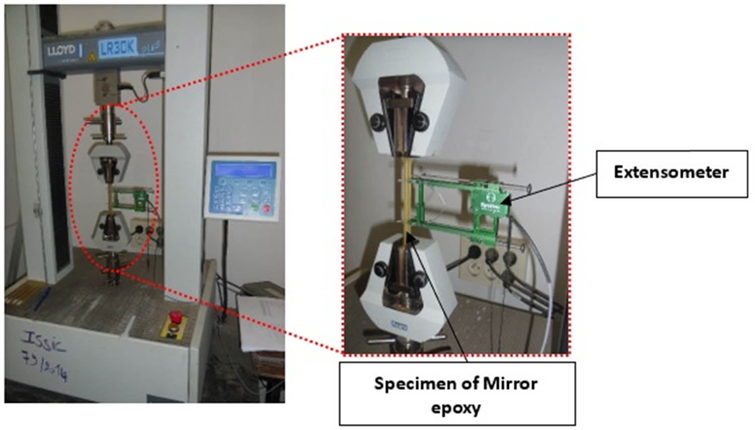
Experimental equipment.

The test specimens were manufactured according to ISO 527-2: 2012 [26]. The specimens were produced by laser cutting a mirror epoxy plate already obtained by molding to avoid roughness along the edges and to have the maximum match [27].

Figure 2 highlights the effect of an increase in the loading speed, revealing a strongly time-dependent behavior of the mirror epoxy resin. Viscoelasticity involves both elastic and viscous behaviors. At higher loading speeds, viscous effects can become more pronounced, affecting material deformation and response. Tensile tests at different speeds make it possible to evaluate the impact of viscosity on the behavior of the material. The viscoelastic zone of a material exhibits both elastic and viscous behavior. By choosing stresses in this area, one can observe how the material deforms over time under constant load, allowing the study of nonlinear viscosity and its impact on material behavior. The stresses 4, 7, 9, 11, and 13 MPa belong to and cover the viscoelastic zone, as well as the strain levels 0.25, 0.5, 0.75, 1, and 1.25%. A loading speed of 1 mm/min with an elastic modulus (E) of 1,500 MPa is chosen, assuming that Poisson’s ratio (ʋ) is constant of the order of 0.3 [28].

Figure 2

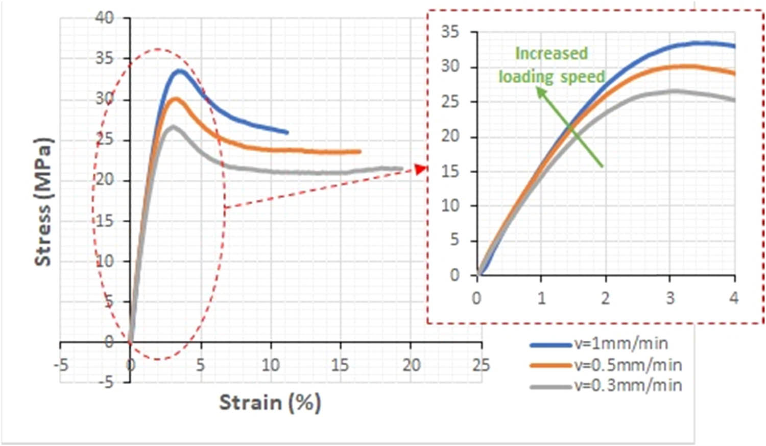
Mirror epoxy tensile tests at different speeds and a temperature of 23°C.

4 Method of resolution of the nonlinear viscoelastic behavior law of creep type

Creep is a phenomenon that describes the time-dependent deformation of a material instantaneously subjected to a constant stress [29,30,31]. Schapery’s viscoelastic formulation is most widely used to model the nonlinear viscoelastic behavior of polymers [32]. Based on the principles of irreversible thermodynamics [33], and in the case of a uniaxial loading, Schapery proposed in his works [34,35,36,37] the nonlinear viscoelastic constitutive law of creep type as follows:

where the coefficients g 0 ( σ ) , g 1 ( σ ) , and g 2 ( σ ) are the nonlinear viscoelastic material parameters, which depend on the level of applied stress ( σ ) .

ψ and ψ * are reduced times expressed as follows:

a σ is a stress σ-dependent factor expressing the reduction in time. For solid viscoelastic materials (polymers) and in the case of isothermal deformation, this factor is equal to 1.

Thus, Eq. (1) becomes

It is interesting to apply this formula for the constant stress creep case and to determine the factors of nonlinearity.

In the case of creep under constant stress,

Let us suppose that g = g 1 ( σ ) g 2 ( σ ) ; then, the new equation is

∆ D ( t ) represents the transient creep flexibility and is an exponential function that can be expressed by a 5-term Prony series. To identify the parameters D i and τ i , it is possible to arbitrarily choose a distribution of the relaxation times τ i according to a power law such that τ i = 10 ⁱ [38]:

where the material constants D i a nd τ i represent the transient flexibility and the relaxation times, respectively, associated with a viscous mechanism. We finally obtain

To determine the nonlinearity coefficients g 0 ( σ ) and g ( σ ) , and by analogy with the iterative procedure of Gmir et al. [23], five constant stress creep tests on mirror epoxy were carried out (Figure 2). Then, for each test (k = 5), we note the strains ε k * ( t j ) associated with the times t _j , with j = 1, …, n (n = 16).

The experimental value of the creep rigidity for test k measured at each time t _j is given by

For each test k,

Thus, the sum over all times tj and all tests k of the differences to the squares of the theoretical values D k ( t ) and the experimental values D k * ( t i ) is determined.

The minimization condition of the difference between the theoretical and experimental rigidity values is

∂ S ∂ D i = 0 for i = 0, …, m.

The result is a linear system of m + 1 (m = 5) equations, which are written in the following matrix form:

with ⨂ denoting the operation between two matrices obtained by the element-by-element multiplication.

The different matrices are as follows:

G = g 00 g 0 … g 0 g 01 g 1 … g 1 … … … … g 0 p g p … g p , a dimension matrix (m + 1) × (p + 1),

A = 1 1 − e − t 1 τ 1 … 1 − e − t 1 τ m 1 1 − e − t 2 τ 1 ⋯ 1 − e − t 2 τ m ⋯ ⋯ ⋯ ⋯ 1 1 − e − t n τ 1 ⋯ 1 − e − t n τ m , a dimension matrix (m + 1) × n,

D * = D 0 * ( t 1 ) D 1 * ( t 1 ) … D p * ( t 1 ) D 0 * ( t 2 ) D 1 * ( t 2 ) … D p * ( t 2 ) … … … … D 0 * ( t n ) D 1 * ( t n ) … D p * ( t n ) , a dimension matrix (p + 1) × n.

The vectors u → and d → are expressed as

The method used to solve this system assumes that the first test is performed at low stress, so the linear behavior law [39,40] can be applied. In this case,

Subsequently, the linear rigidity D 0 l ( t ) is written as

Therefore, the boundary conditions are expressed in the following form:

At the instant t = 0, D 0 l = D 0 , ε 0 l ( 0 ) = σ 0 D 0 .

At the instant t = ∞ ,

For the other k = 1, …, p tests (p = 4), the behavior of the material is nonlinear. The rigidities at the extreme times t = 0 and t = ∞ are expressed by

For a first approximation,

In this approach, t n = t → ∞. The strains measured at times 0 and t n are written as

Then, the outcome is as follows:

Using the least-squares method for each test k, the result is

The minimization of S k is obtained when

The problem boils down to the following matrix:

The vectors g → k and d → k * are as follows:

The matrix A g of dimension 2 × n is written as

From Figure 3, ε k * ( t j ) associated with times t _j is determined. Then, the experimental value of the creep stiffness D k * ( t i ) is determined. Next, minimize the difference between the theoretical and experimental values of the stiffnesses in order to obtain [ ( G t · G ) ⨂ ( A t · A ) ] d → = [ G t ⨂ ( A t · D * ) ] u → .

Figure 3

Resolution algorithm of nonlinearity coefficients of Schapery’s law [28].

To solve this system, we can apply the linear constitutive law since the stress is low ( σ = 4 MPa ) ). In this case, g 00 = g 0 = 1 . For the other constraints ( σ = 7 , 9 , 11 , 13 MPa ) , the behavior is nonlinear and the rigidities at extreme times make it possible to obtain

Then, the calculation of d → is possible d i → = [ G t ⨂ ( A t · D * ) ] u → [ ( G t · G ) ⨂ ( A t · A ) ] for the first iteration (i = 1). However, a new minimization between the theoretical and experimental rigidity makes it possible to obtain ( A g t · A g ) g → k = A g t d → k * to calculate the new values of g → k = g 0 k g k , which allows us to calculate d i + 1 → = [ G t ⨂ ( A t · D * ) ] u → [ ( G t · G ) ⨂ ( A t · A ) ] .

The algorithm continues iterating until this difference ( d i + 1 − d i ) becomes less than a 10⁻⁴ [41,42] threshold, indicating that the coefficients have converged to stable values. Once this condition is verified, the algorithm programmed on MATLAB stops and the nonlinearity coefficients g 0 k and g k of the Schapery model are considered to be determined with acceptable precision. Finally, we can write and trace the Schapery model curve.

5 Method of resolution of the nonlinear viscoelastic behavior law of relaxation type

Based on the same laws of thermodynamics, Schapery developed the behavior law for a relaxation-type loading as follows:

where h 0 * ( ε ) , h 1 ( ε ) , and h 2 ( ε ) are nonlinearity factors, depending on the strain ε.

ϑ and ϑ * are reduced times expressed by

where a ε is a factor dependent on the strain ε, which expresses the reduction in time. For solid viscoelastic materials (polymers) and in the case of isothermal deformation, this factor is equal to 1.

Eq. (20) is then written in the following form:

It is interesting to apply this formula on the case of relaxation under constant strain and to determine the nonlinearity factors. In the case of relaxation under constant strain, we have

Let us suppose that h * ( ε ) = h 1 ( ε ) h 2 ( ε ) . Then, we have

∆ E ( t ) is a function expressed as an exponential series:

ultimately leading to

which can also be written in the following form:

To determine the nonlinearity coefficients h 0 ( ε ) and h ( ε ) , the following iterative procedure is adopted: Perform five constant strain relaxation tests on mirror epoxy (Figure 3); then, for each test k (k = 5), the stresses σ k * ( t j ) associated with times t _j , with j = 1, …, N (n = 16) are obtained.

The experimental value of the relaxation modulus for test k measured at each instant t _j is given by

For each test k, we can write

Thus, the sum over all times t _j and all tests k of the differences to the squares of the theoretical values E k ( t ) and the experimental values E k * ( t j ) is determined:

To minimize the difference between the theoretical and experimental values of the rigidities, it is necessary that

A linear system of (m + 1) equations is obtained, written in the following matrix form:

The different matrices are as follows:

H = h 00 h 0 … h 0 h 01 h 1 … h 1 … … … … h 0 p h p … h p , a dimension matrix (m + 1) × (p + 1) (p = 4),

B = 1 − 1 + e − t 1 τ 1 … − 1 + e − t 1 τ m 1 − 1 + e − t 2 τ 1 ⋯ − 1 + e − t 2 τ m ⋯ ⋯ ⋯ ⋯ 1 − 1 + e − t n τ 1 ⋯ − 1 + e − t n τ m , a dimension matrix (m + 1) × n,

E * = E 0 * ( t 1 ) E 1 * ( t 1 ) … E p * ( t 1 ) E 0 * ( t 2 ) E 1 * ( t 2 ) … E p * ( t 2 ) … … … … E 0 * ( t n ) E 1 * ( t n ) … E p * ( t n ) , a dimension matrix (p + 1) × n.

The vectors u → and e → are expressed by

The method used to solve this system is to assume that the first test is done at low strain and so we can apply the linear behavior law [43]. In this case,

Then, the linear relaxation modulus E 0 l ( t ) can be written as

Then,

At the instant t = 0, E 0 l ( 0 ) = E 0 , σ 0 l ( 0 ) = ε 0 E 0 .

At the instant t = ∞ , E 0 l ( ∞ ) = E 0 − ∑ i = 1 m E i , σ 0 l ( ∞ ) = ε 0 E 0 l ( ∞ ) .

For the other k = 1, …, p tests, the behavior of the material is nonlinear. The relaxation module at the extreme times t = 0 and t = ∞ is expressed by

A first approximation

In this approach, we set t n = t → ∞ . The stresses measured at times 0 and t n are written as

Then,

Using the least-squares method for each test k,

The minimization of S _k is obtained when

The problem boils down to the following matrix:

The vectors h → k and e → k * are as follows:

The matrix B h of dimension 2 × n is written as

With the approximate values of h 0 k and h k calculated using relations (34), we determine the relaxation modulus E k ( t ) of Eq. (29), and with Eq. (39), we determine the new values of h 0 k and h k . This iteration is repeated until the convergence of the procedure, which is programmed in MATLAB.

The algorithm for solving the coefficients of nonlinearities is represented in Figure 4.

Figure 4

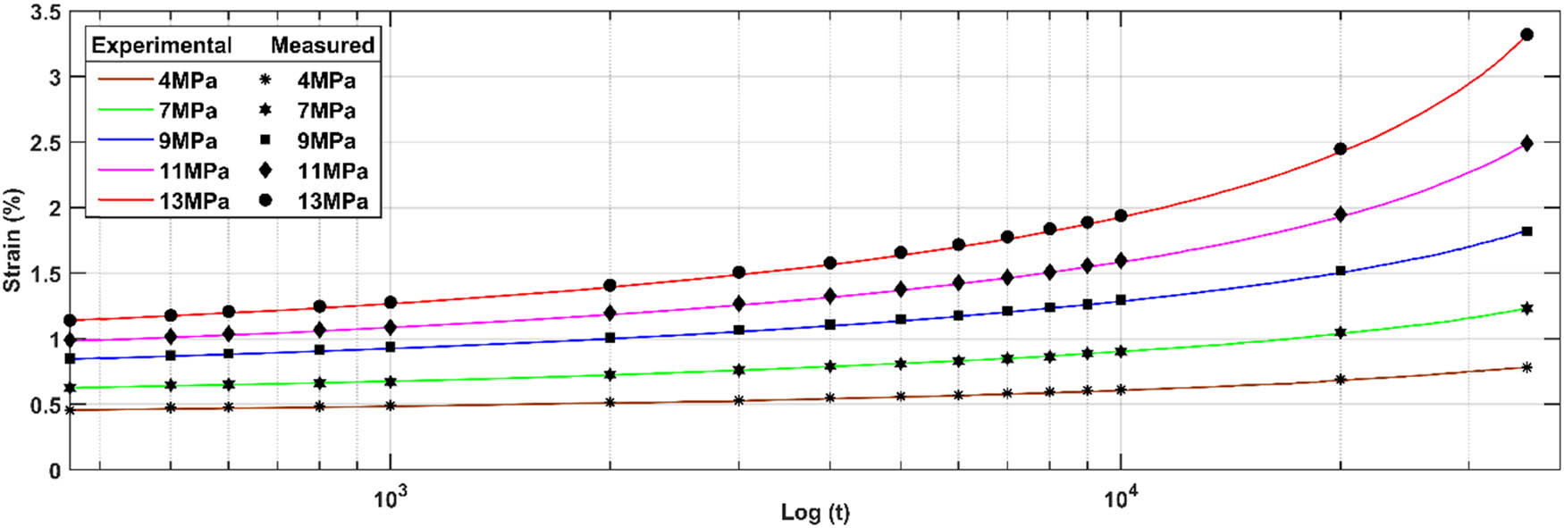
Experimental and measured creep curves of mirror epoxy with logarithmic axis.

5.1 Results and discussion

5.1.1 Creep case

The identification of the parameters ( D i , τ i ) , which is based on the method of least squares, allowed us to obtain the optimal couples ( D i , τ i ) , as shown in Table 1. The results of the nonlinear coefficients as a function of the applied loads are shown in Figure 5.

Table 1

Parameters D _i and τ i

	D i (MPa)	τ i (s)
D 0	0.1237 × 10−2	.
D 1	−0.0171 × 10−2	10
D 2	0.0069 × 10−2	100
D 3	0.0135 × 10−2	1,000
D 4	0.0065 × 10−2	10,000
D 5	0.2179 × 10−2	100,000

Figure 5

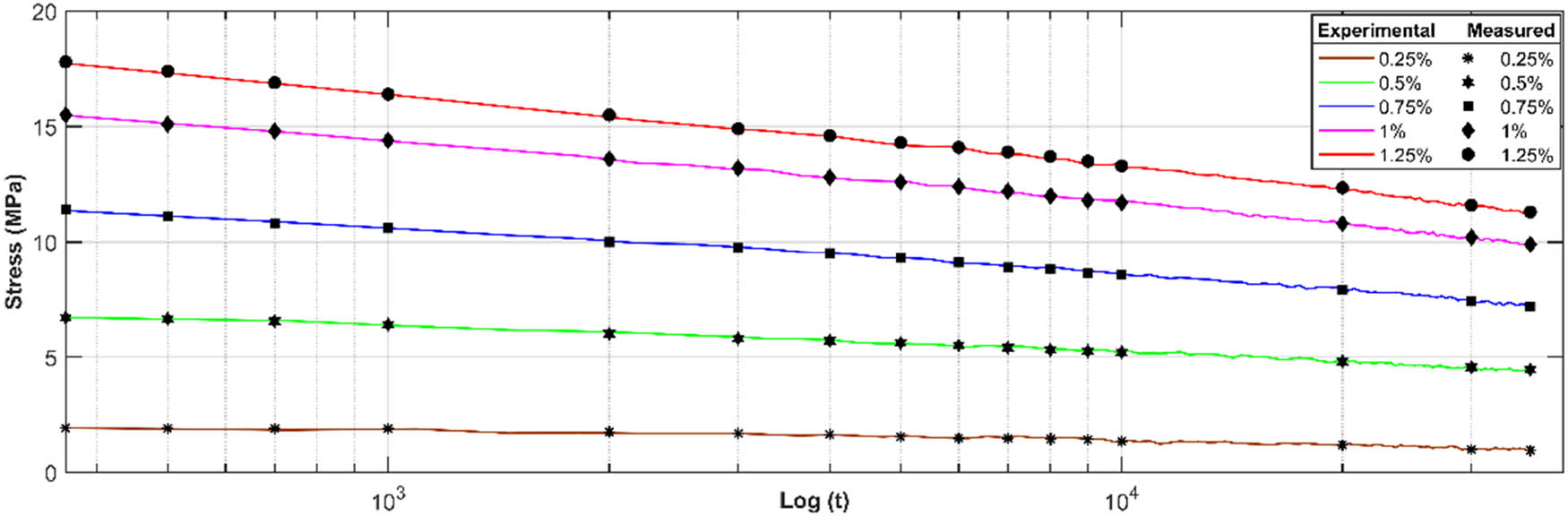
Experimental and measured relaxation curves of mirror epoxy with logarithmic axis.

An interpolation of the nonlinearity coefficients using second-degree polynomials is necessary to use them later in the numerical simulation in order to be compared with the experimental one:

g = f ( σ ) = 1 for σ ≤ 4 MPa ,

g = 0.0116 × σ 2 − 0.07989 × σ + 1.121 for σ > 4 MPa ,

g 0 = f ( σ ) = 1 for σ ≤ 4 MPa ,

g 0 = 0.001949 × σ 2 − 0.05842 × σ + 1.201 for σ > 4 MPa .

Figure 6 allows us to visualize the variation in the experimental deformations of the mirror epoxy at different loading levels (4, 7, 9, 11, and 13 MPa). The deformation increases with time and the material continues to deform gradually over time in response to different applied stresses. An increase in the applied stress generally results in an increase in strain over time, resulting in a greater slope on the strain curves.

Figure 6

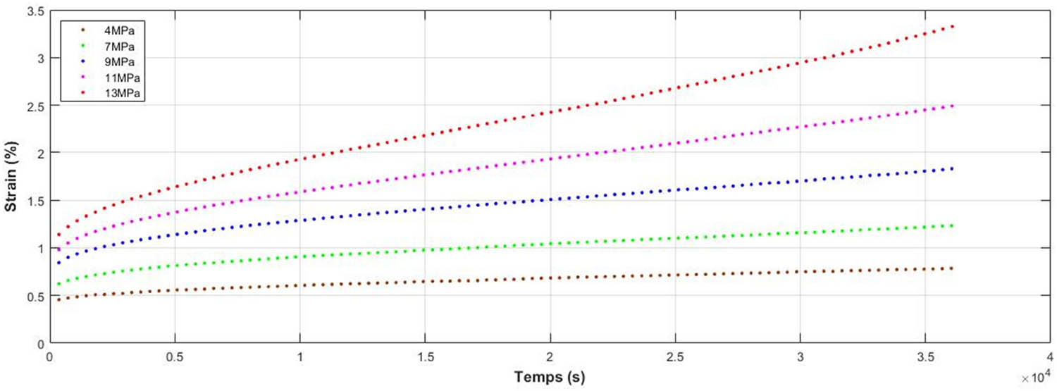
Variation of the experimental deformations of the mirror epoxy at different loading levels (4, 7, 9, 11, and 13 MPa).

This remarkable increase in slope indicates a higher strain rate, which is consistent with the viscoelastic behavior of the material. At relatively low stress levels (4 MPa), the viscoelastic behavior is linear, and the material response is proportional to the magnitude of the applied stress. As the stress level increases (7, 9, 11, and 13 MPa), the nonlinearities in the viscoelastic behavior can become more pronounced. This can manifest itself in effects such as time dependence of strain, variable strain rates, and viscoelastic responses, i.e., not proportional to the applied stress.

To confirm this interpretation, it is necessary to construct isochronous [44] curves in order to experimentally determine the nonlinearity interval of the viscoelasticity of the material studied. These curves are obtained by recording the viscoelastic deformation for each stress level, at a given time. The viscoelastic deformation is recorded for a period of 1 and 10 h. For the two moments considered, we notice in Figure 7 a strong nonlinearity from a threshold close to 4 MPa. This result allows us to consider that for creep stresses greater than 4 MPa, the viscoelastic behavior can be described as nonlinear.

Figure 7

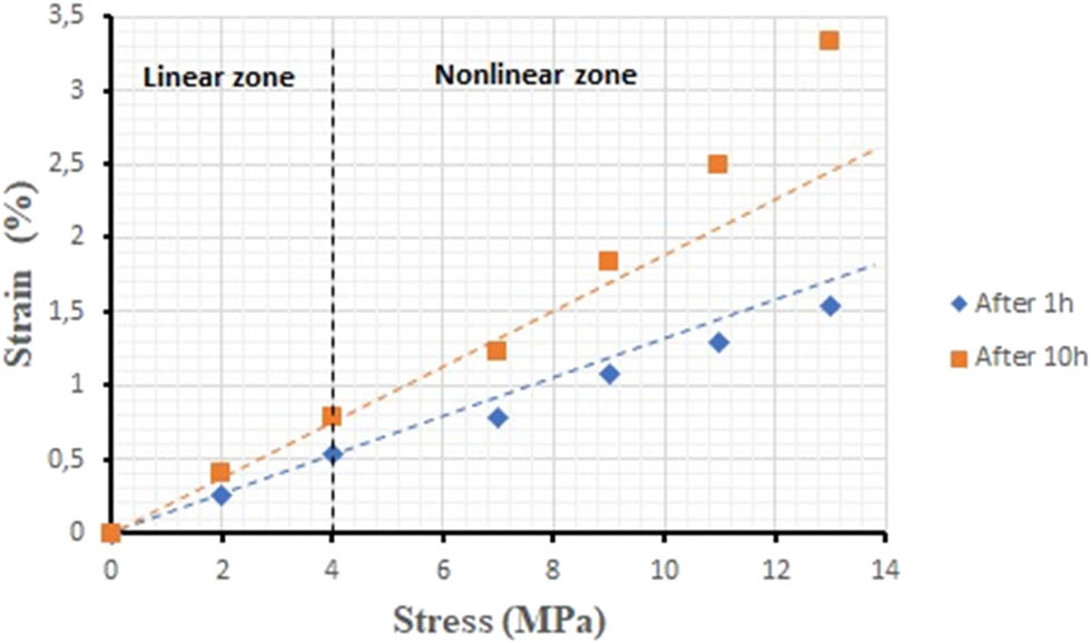
Isochronous curves at two given times and the identification of the nonlinearity limit of the creep-type viscoelasticity of mirror epoxy.

After determining the creep-type nonlinearity parameters of the material studied in Figure 8 and the parameters of the prony series ( D i , τ i ) in Table 1, the tracing of Schapery’s law is possible. A remarkable consistency is observed in Figure 9 between the variations of the experimental strain at different stress levels and this model.

Figure 8

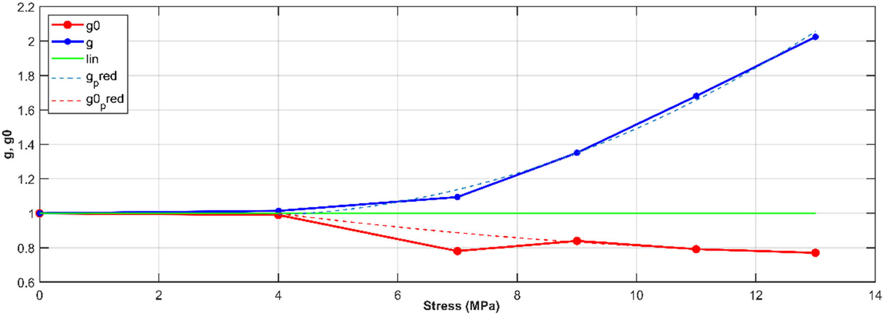
The nonlinearity coefficients of the creep-type Schapery law of mirror epoxy.

Figure 9

Variation of experimental and numerical deformations of mirror epoxy at different stress levels (4, 7, 9, 11, and 13 MPa).

Schapery’s law is effectively used to model linear viscoelastic behavior, particularly in the case of low-stress levels. At 4 MPa, the nonlinear parameters are equal to 1, and the behavior is linear. At high stress levels (7, 9, 11, and 13 MPa), Schapery’s law can also be used to describe the nonlinear viscoelastic behavior of materials under study. In this stress range, where strain is large and loading times longer, nonlinear viscoelastic effects become significant. Schapery’s law allows us to predict these nonlinear behaviors by including nonlinear creep-type coefficients g and g ₀, which take into account the dependence of the viscoelastic response on stress and time.

On the microscopic scale, intermolecular bond tensions play a crucial role. In epoxy, polymer chains are held together by intermolecular bonds. When these bonds are subjected to stress, they can deform, break, or rearrange, resulting in the viscoelastic behavior of the material. However, beyond the linearity threshold, deformations can become irreversible due to the breakdown of intermolecular bonds or their reorganization, which leads to nonlinear viscoelastic behavior [45].

5.1.2 Relaxation case

The identification of the parameters ( E i , τ i ) , which is based on the method of least squares, makes it possible to obtain the couples ( E i , τ i ) optimal, as shown in Table 2. Also, the results of the nonlinear coefficients as a function of the applied strain are shown in Figure 9.

Table 2

Parameters E i and τ i

	E i	τ i
E0	6.8822 × 10−2
E1	−3.1959 × 10−2	10
E2	1.6271 × 10−2	100
E3	1.4841 × 10−2	1,000
E4	2.0405 × 10−2	10,000
E5	2.8984 × 10−2	100,000

An interpolation of the nonlinearity coefficients using second-degree polynomials is necessary to use them later in the numerical simulation in order to be compared with the experimental one.

h = f ( ε ) = 1 for ε ≤ 0.25 % ,

h = − 0 , 8673 × ε 2 + 1 , 6137 × ε + 0 , 6671 for ε > 0.25 % ,

h 0 = f ( ε ) = 1 for ε ≤ 0.25 % ,

h 0 = − 2 , 3143 × ε 2 + 4 , 2257 × ε + 0 , 1427 for ε > 0.25 % .

Other mechanical tests make it possible to highlight the time-dependent behavior of materials, such as relaxation, to confirm the viscoelastic behavior of the material studied. Figure 10 allows one to visualize the evolution of the stress as a function of time at different deformation levels (0.25, 0.5, 0.75, 1 and 1.25%). The results indicate that during these tests, the material undergoes stress relaxation, confirming a very time-dependent behavior. At relatively low strain levels (0.25%), the relaxation rate is very high, the curve reaches a steady state in a very short time, and the behavior tends towards linearity. As the level of strain increases (0.5, 0.75, 1, and 1.25%), the nonlinearities of the viscoelastic behavior can become more pronounced. This can manifest itself in effects, such as stress dependence, on time variable strain rates.

Figure 10

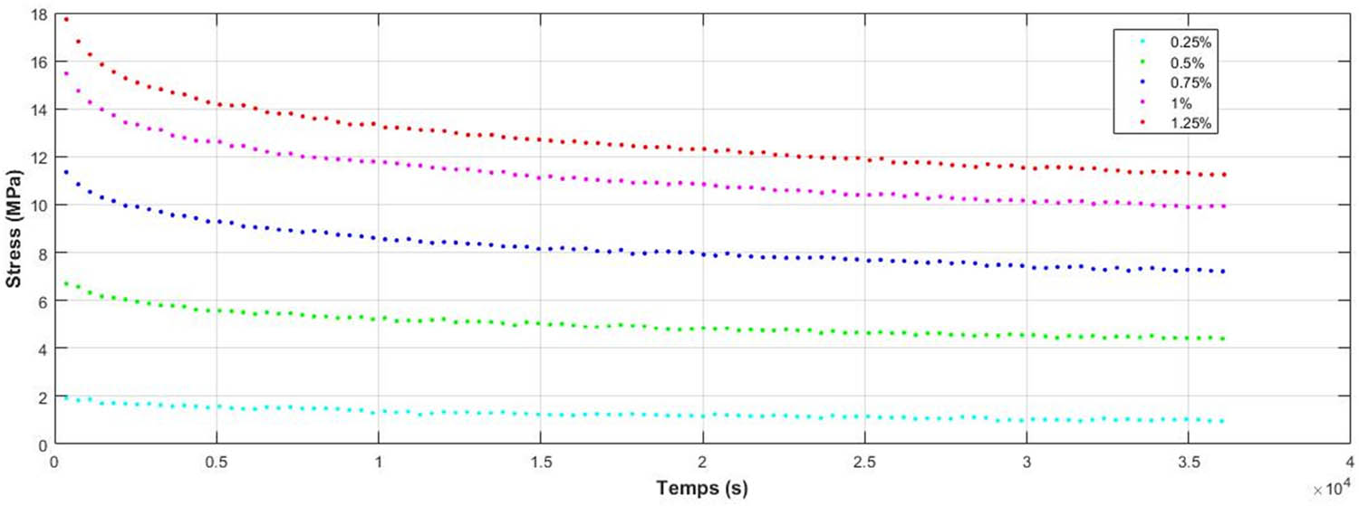
Experimental relaxation curves of mirror epoxy at different strain levels (0.25, 0.5, 0.75, 1 and 1.25%).

To confirm this interpretation, it is necessary to construct isothermal curves in order to experimentally determine the nonlinearity interval of the viscoelasticity of the material studied. These curves are obtained by recording the stresses for each level of strain at a given time. The constraints are noted for times 1 and 10 h. For the two moments considered, we observe in Figure 11 a strong nonlinearity from a threshold close to 0.25%. This result allows us to consider that for strain greater than 0.25%, the relaxation-type viscoelastic behavior can be qualified as nonlinear.

Figure 11

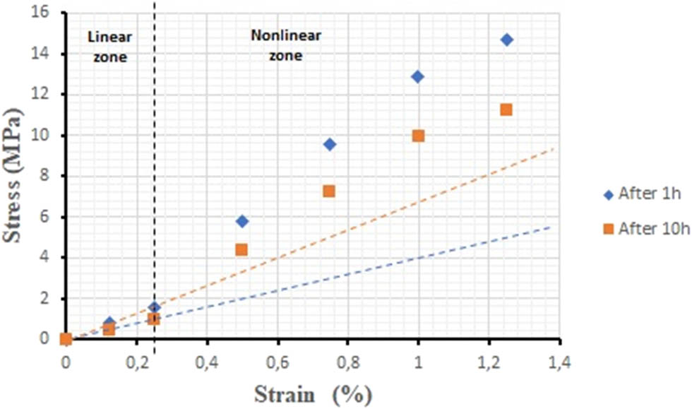
Isothermal curves at two given times and the identification of the nonlinearity limit of the relaxation type viscoelasticity of the mirror epoxy.

After determining the relaxation-type nonlinearity parameters of the material studied in Figure 12 and the parameters of the Prony series ( E i , τ i ) in Table 2, the tracing of Schapery’s law is possible. A remarkable consistency in seen Figure 13 between the variations of experimental stresses at different strain levels and this model.

Figure 12

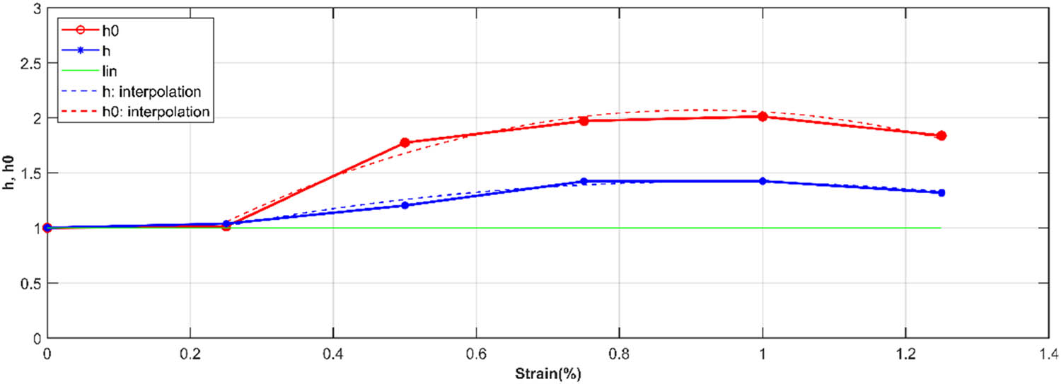
The coefficients of nonlinearity of Schapery law of the relaxation type of mirror epoxy.

Figure 13

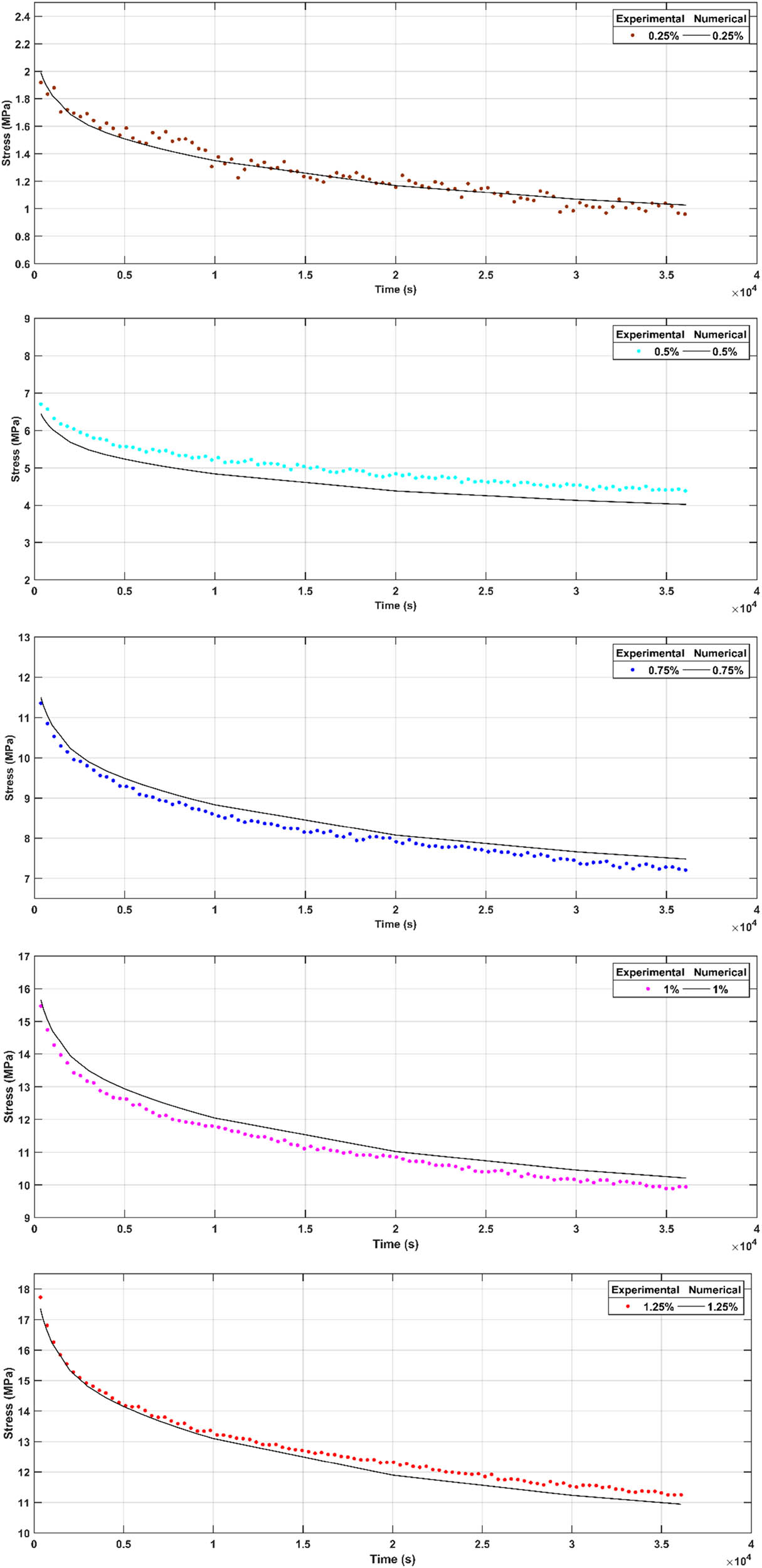
Variation in the experimental and numerical stress of mirror epoxy at different strain levels (0.25, 0.5, 0.75, 1, and 1.25%).

Schapery’s law is effectively used to model linear viscoelastic behavior, particularly in the case of low strain levels. At 0.25%, the nonlinear parameters are equal to 1, and the behavior is linear. At high strain levels (0.5, 0.75, 1, and 1.25%), Schapery’s law can also be used to describe the nonlinear viscoelastic behavior of materials studied. In this strain range, where the loads are large and the strain times are longer, the nonlinear viscoelastic effects become significant. Schapery’s law makes it possible to predict these nonlinear behaviors by including nonlinear relaxation-type coefficients h and h ₀, which take into account the dependence of the viscoelastic response on strain and time.

On the microscopic scale, relaxation is associated with molecular rearrangements and the reduction of internal tensions in the material.

6 Conclusion

The long-term creep tests on mirror epoxy specimens at different stress levels (4, 7, 9, 11, and 13 MPa) allowed us to determine numerically the coefficients of nonlinearity of the creep type. A remarkable consistency between the variations in the experimental strains at different stress levels and the Schapery numerical model allowed us to conclude that this describes the nonlinear viscoelastic behavior of the creep type of mirror epoxy.

Likewise, the long-term relaxation tests carried out under the same conditions on the same specimens at different levels of strains (0.25, 0.5, 0.75, 1, and 1.25%) allowed us to determine numerically the coefficients of nonlinearity of relaxation type. An excellent agreement was observed between the variations of the experimental stresses at different strain levels and the Schapery numerical model.

Thus, this model satisfactorily describes the nonlinear viscoelastic behavior of the creep type and that of the relaxation type, which proves the validation of this model for the real viscoelastic behavior of the studied material.

Validation of the Schapery model to describe the nonlinear viscoelastic behavior of mirror epoxy used in 3D flooring can provide important information to address the low-velocity mass impact phenomenon. This could lead to more resilient and safer flooring designs in various applications.

References

[1] Amaro AM, Bernardo L, Pinto DG, Lopes S, Rodrigues J. The influence of curing agents in the impact properties of epoxy resin nanocomposites. Compos Struct. 2017;174:26–32.10.1016/j.compstruct.2017.04.050Search in Google Scholar
[2] Verma A, Negi P, Singh VK. Experimental investigation of chicken feather fiber and crumb rubber reformed epoxy resin hybrid composite: Mechanical and microstructural characterization. J Mech Behav Mater. 2018;27(3–4):1–24.10.1515/jmbm-2018-0014Search in Google Scholar
[3] Sukanto H, Raharjo WW, Ariawan D, Triyono J. Investigation of cycloaliphatic amine-cured bisphenol-A epoxy resin under quenching treatment and the effect on its carbon fiber composite lamination strength. J Mech Behav Mater. 2023;32:1.10.1515/jmbm-2022-0266Search in Google Scholar
[4] Aldosari MA, Sawsan S, Darwish SS, Adam MA, Elmarzugi NA, Ahmed SM. Re-assembly of archaeological massive limestones using epoxy resin modified with nanomaterials—part 1: experimental. Green Sustainable Chem. 2020;10(1):24–38.10.4236/gsc.2020.101003Search in Google Scholar
[5] Jin FL, Park SJ. Recent advances in carbon-nanotube-based epoxy composites. Carbon Lett. 2013;14(1):1–13.10.5714/CL.2012.14.1.001Search in Google Scholar
[6] Park SJ, Kim MH, Lee JR, Choi S. Effect of fiber-polymer interactions on fracture toughness behavior of carbon fiber-reinforced epoxy matrix composites. J Colloid Interface Sci. 2000;228(2):287–91.10.1006/jcis.2000.6953Search in Google Scholar PubMed
[7] Keziz A, Heraiz M, Sahnoune F, Rasheed M. Characterization and mechanisms of the phase’s formation evolution in sol-gel derived mullite/cordierite composite. Ceram Int. 2023;49(20):32989–3003.10.1016/j.ceramint.2023.07.275Search in Google Scholar
[8] Kherifi D, Keziz A, Rasheed M, Oueslati A. Thermal treatment effects on Algerian natural phosphate bioceramics: A comprehensive analysis. Ceram Int. 2024;50(17):30175–87.10.1016/j.ceramint.2024.05.317Search in Google Scholar
[9] Sellam M, Rasheed M, Azizii S, Saidani T. Improving photocatalytic performance: Creation and assessment of nanostructured SnO2 thin films, pure and with nickel doping, using spray pyrolysis. Ceram Int. 2025;50(12):20917–35.10.1016/j.ceramint.2024.03.094Search in Google Scholar
[10] Keziz A, Rasheed M, Heraiz M, Sahnoune F, Latif A. Structural, morphological, dielectric properties, impedance spectroscopy and electrical modulus of sintered Al6Si2O13–Mg2Al4Si5O18 composite for electronic applications. Ceram Int. 2023;49(23):37423–34.10.1016/j.ceramint.2023.09.068Search in Google Scholar
[11] Alshalal I, Al-Zuhairi HMI, Abtan AA, Rasheed M, Asmail MK. Characterization of wear and fatigue behavior of aluminum piston alloy using alumina nanoparticles. J Mech Behav Mater. 2023;32(1):20220280.10.1515/jmbm-2022-0280Search in Google Scholar
[12] Al Zubaidi FN, Asaad LM, Alshalal I, Rasheed M. The impact of zirconia nanoparticles on the mechanical characteristics of 7075 aluminum alloy. J Mech Behav Mater. 2023;32(1):20220302.10.1515/jmbm-2022-0302Search in Google Scholar
[13] Pabel MM JA, Agudo JAR, Gude M. Measuring and understanding cure-dependent viscoelastic properties of epoxy resin: A review. Polym Test. 2022;114:107701.10.1016/j.polymertesting.2022.107701Search in Google Scholar
[14] Nguyen HG. Micromechanical approach for modeling the elastoplastic behavior of composites: application to resin mortars [dissertation]. France: University of Cergy-Pontoisepp; 2008.Search in Google Scholar
[15] Saleh NJ, Razak AAA, Tooma MA, Aziz ME. A study mechanical properties of epoxy resin cured at constant curing time and temperature with different hardeners. Eng Tech J. 2011;29(9):1804–18.10.30684/etj.29.9.15Search in Google Scholar
[16] Pereira AAC, D’Almeida JRM. Effect of the hardener to epoxy monomer ratio on the water absorption behavior of the DGEBA/TETA epoxy system. Polimeros. 2016;26(1):30–7.10.1590/0104-1428.2106Search in Google Scholar
[17] Leaderman H. Elastic and creep properties of filamentous materials [dissertation]. England: University of cambridge; 1941.Search in Google Scholar
[18] Bernstein B, Kearsley EA, Zapas JL. A study of stress relaxation with finite strain. Rubber Chem Technol. 1963;7(1):391.10.1122/1.548963Search in Google Scholar
[19] Green AE, Rivlin RS. The mechanics of non-linear materials with memory. Arch Ration Mech Anal. 1959;4(1):387–404.10.1007/BF00281398Search in Google Scholar
[20] Jafaripour M, Behrooz FT. Creep behavior modeling of polymeric composites using Schapery model based on micro-macromechanical approaches. Eur J Mech A/Solids. 2020;81:103963.10.1016/j.euromechsol.2020.103963Search in Google Scholar
[21] Sun T, Yu C, Yang W, Zhong J, Xu Q. Experimental and numerical research on the nonlinear creep response of polymeric composites under humid environments. Compos Struct. 2020;251:112673.10.1016/j.compstruct.2020.112673Search in Google Scholar
[22] Zink T, Kehrer L, Hirschberg V, Wilhelm M, Böhlke T. Nonlinear Schapery viscoelastic material model for thermoplastic polymers. J Appl Polym Sci. 2022;139(17):1–7.10.1002/app.52028Search in Google Scholar
[23] Gmir F, Aloui A, Haddar M. A nonlinear creep of PMMA under cyclic loading. IJESAT. 2012;2(5):1192–8.Search in Google Scholar
[24] Cruz R, Correia L, Fonseca SC, Cruz JS. Effects of the preparation, curing and hygrothermal conditions on the viscoelastic response of a structural epoxy adhesive. Int J Adhes Adhes. 2021;110:102961.10.1016/j.ijadhadh.2021.102961Search in Google Scholar
[25] Lu F, Hou Y, Zhang B, Huang L, Qin F, Song D. Study on the ratchetting behavior of glass fiber-reinforced epoxy composites: Experiment and theory. Polym Test. 2023;117:107875.10.1016/j.polymertesting.2022.107875Search in Google Scholar
[26] Silva P, Valente T, Azenha M, Cruz JS, Barros J. Viscoelastic response of an epoxy adhesive for construction since its early ages: Experiments and modelling. Compos Part B Eng. 2017;116:266–77.10.1016/j.compositesb.2016.10.047Search in Google Scholar
[27] Hu J, Chen W, Fan P, Gao J, Fang G, Cao Z, et al. Epoxy shape memory polymer (SMP): Material preparation, uniaxial tensile tests and dynamic mechanical analysis. Polym Test. 2017;62:335–41.10.1016/j.polymertesting.2017.07.001Search in Google Scholar
[28] Gmir F. Static and dynamic analysis of cracked structures in viscoelastic materials [dissertation]. Tunisia: University of Sfax; 2014.Search in Google Scholar
[29] Gu HH, Wang RZ, Zhu SP, Wang XW, Wang DM, Zhang GD, et al. Machine learning assisted probabilistic creep-fatigue damage assessment. Int J Fatigue. 2022;156:106677.10.1016/j.ijfatigue.2021.106677Search in Google Scholar
[30] Wang RZ, Gu HH, Zhu SP, Li KS, Wang J, Wang XW, et al. A data-driven roadmap for creep-fatigue reliability assessment and its implementation in low-pressure turbine disk at elevated temperatures. Reliab Eng Syst Saf. 2022;225:108523.10.1016/j.ress.2022.108523Search in Google Scholar
[31] Meng D, Yang S, Yang H, De Jesus AMP, Correia J, Zhu SP. Intelligent-inspired framework for fatigue reliability evaluation of offshore wind turbine support structures under hybrid uncertainty. Ocean Eng. 2024;307:118213.10.1016/j.oceaneng.2024.118213Search in Google Scholar
[32] Schapery RA. On the characterization of nonlinear viscoelastic materials. Polym Eng Sci. 1969;9(4):295–310.10.1002/pen.760090410Search in Google Scholar
[33] Gacem H, Chevalier Y, Dion JL, Soula M, Rezgui B. Long term prediction of nonlinear viscoelastic creep behaviour of elastomers: Extended Schapery model. Mec Ind. 2008;9(5):407–16.10.1051/meca/2009003Search in Google Scholar
[34] Schapery RA. A theory of nonlinear thermoviscoelasticity based on irreversible thermodynamics. Proc. 5th U.S. National Congress of applied mechanics. March, lafayette: 1966.Search in Google Scholar
[35] Schapery RA. An engineering theory of nonlinear. Int J Solids Struct. 1966;2(3):407–25.10.1016/0020-7683(66)90030-8Search in Google Scholar
[36] Schapery RA. Application of thermodynamics to thermomechanical, fracture, and birefringent phenomena in viscoelastic media. J Appl Phys. 1964;35(5):1451–65.10.1063/1.1713649Search in Google Scholar
[37] Bruggeman M, Yang Q, Zaoutsos S, Boulpaep F, Dumortier S, Cardon HA. Study of the non-linear meterial behaviour of fidredux 920-C-TS-5-42. J Mech Behav Mater. 1998;1:1–6.10.1515/JMBM.1998.9.1.91Search in Google Scholar
[38] Albouy W. On the contribution of visco-elasto-plasticity to the fatigue behavior of thermoplastic and thermosetting matrix composites [dissertation]. France: Normandy University; 2013.Search in Google Scholar
[39] Albouy W, Vieille B, Taleb L. Experimental study of the creep/recovery behavior of C/TP composites and evaluation of the Schapery model. 20th French Congress of Mechanics. Besançon. Association Française de Mécanique; 2011. Aug 29 to September 2.Search in Google Scholar
[40] Chen Y, Smith LV. A nonlinear viscoelastic–viscoplastic model for adhesives. Mech Time-Depend Mater. 2021;25(4):565–79.10.1007/s11043-020-09460-2Search in Google Scholar
[41] Akoussan K. Modeling and design of viscoelastic composite structures with high damping power [dissertation]. France: University of Lorraine; 2015.Search in Google Scholar
[42] Sabri LA, Al-Tamimi ANJ, Alshamma FA, Mohammed MN, Salloomi KN, Abdullah OI. Performance evaluation of nonlinear viscoelastic materials using finite element method. Int J Appl Mech Eng. 2024;29(1):142–58.10.59441/ijame/184138Search in Google Scholar
[43] Pupure L, Varna J, Joffe R. Applications and limitations of non-linear viscoelastic model for simulation of behaviour of polymer composites. 20th International Conference on Composite Materials. Copenhagen: 2015 July.Search in Google Scholar
[44] Abdessemed K, Allaoui O, Guerira B, Ghelani L. Characterization of the thermal, water absorption, and viscoelastic behavior of short date palm fiber reinforced epoxy. Mech Time-Depend Mater. 2023;1–25.10.1007/s11043-023-09656-2Search in Google Scholar
[45] Bouvet G. Relationships between microstructure and physicochemical and mechanical properties of model epoxy coatings [dissertation]. France: Rochelle university Rochelle; 2014.Search in Google Scholar
© 2024 the author(s), published by De Gruyter
This work is licensed under the Creative Commons Attribution 4.0 International License.
Articles in the same Issue
- Research Articles
- Evaluation of the mechanical and dynamic properties of scrimber wood produced from date palm fronds
- Performance of doubly reinforced concrete beams with GFRP bars
- Mechanical properties and microstructure of roller compacted concrete incorporating brick powder, glass powder, and steel slag
- Evaluating deformation in FRP boat: Effects of manufacturing parameters and working conditions
- Mechanical characteristics of structural concrete using building rubbles as recycled coarse aggregate
- Structural behavior of one-way slabs reinforced by a combination of GFRP and steel bars: An experimental and numerical investigation
- Effect of alkaline treatment on mechanical properties of composites between vetiver fibers and epoxy resin
- Development of a small-punch-fatigue test method to evaluate fatigue strength and fatigue crack propagation
- Parameter optimization of anisotropic polarization in magnetorheological elastomers for enhanced impact absorption capability using the Taguchi method
- Determination of soil–water characteristic curves by using a polymer tensiometer
- Optimization of mechanical characteristics of cement mortar incorporating hybrid nano-sustainable powders
- Energy performance of metallic tubular systems under reverse complex loading paths
- Enhancing the machining productivity in PMEDM for titanium alloy with low-frequency vibrations associated with the workpiece