Mechanical behavior of designed AH32 steel specimens under tensile loading at low temperatures: Strength and failure assessments based on experimentally verified FE modeling and analysis
-
Muhammad Fauzan Arfandi Ahzhan
 ,
Teguh Muttaqie
,
Teguh Muttaqie

Abstract
This research investigates the mechanical behavior and performance of AH32 steel when subjected to low temperatures, particularly in the context of ship hull structures operating in cryogenic environments. The study uses experimental procedures and advanced numerical simulations through ABAQUS CAE to evaluate vital mechanical properties such as Young’s modulus, yield stress, ultimate tensile strength, and fracture toughness across temperatures ranging from 20 to −160°C. The results reveal a consistent trend of increasing strength and decreasing ductility at lower temperatures, with validation achieved through an error margin of less than 10%. The findings underscore the material’s suitability for cryogenic applications but highlight the potential for brittle fracture, necessitating careful design considerations in Arctic or liquefied natural gas transport conditions. However, the study is limited to specific geometric configurations and loading conditions, suggesting that future research should explore additional geometries, fatigue behavior, and long-term performance under varying environmental conditions to assess the material’s viability in extreme environments fully.
1 Introduction
Liquefied Natural Gas (LNG) stands out as a promising alternative energy source due to its lower greenhouse gas emissions compared to traditional fossil fuels like coal and oil [1,2,3,4,5]. Primarily composed of methane, natural gas is highly efficient and burns cleanly, producing minimal nitrogen and sulfur emissions [6,7,8]. LNG is created by transforming natural gas into a liquid state by cooling it to −161°C (−259°F). The process reduces it to 1/600th of its original un-liquified volume and half the weight of water, making it easier to store and transport [9,10,11,12]. This conversion has enabled LNG to find applications in various industrial sectors, including power generation, shipping, and as an alternative fuel source, thereby becoming an essential part of the global energy market [13,14,15,16,17]. LNG generates electricity in power plants, providing a lower-carbon alternative to coal. It provides grid stability and flexibility, helping to address the intermittency of renewable power sources in electricity generation. LNG and natural gas significantly enable energy transition and quickly switch from dirtier energy sources like coal or heavy fuels to a cleaner alternative. Natural gas emits 45–55% lower greenhouse gas emissions than coal in power generation. In the industrial sector, LNG and natural gas provide a clean solution to those industrial sectors that need high-calorific fuel in their production process and are the most difficult to electrify. In developing economies, it will replace traditional biomass in heating and cooking, helping to reduce the health impacts of localized emissions from other fuels. In the transport sector, LNG has also shown a significant reduction in emissions (both greenhouse and particulate) compared to traditional fuels and is helping diversify the fuel mix and reduce air pollution as a fuel for heavy-duty road transport and shipping [18]. The European Commission’s plan to boost its energy resilience rests on diversifying gas supplies while continuing to boost renewables and improve energy efficiency. The sudden surge in demand for LNG has been felt worldwide, not least in Asia, which has been LNG’s core market for years. The scramble for LNG has left some Asian countries priced out of the market; in a highly unusual development, a recent $1 billion LNG purchase tender by state-owned Pakistan LNG did not receive a single bid. The same happened in India. Other countries are turning to coal to meet their energy needs without LNG being available on the spot market [19].
The growing demand for LNG is paralleled by the expansion of global trade [20]. LNG is transported mainly via pipelines and carriers [21]. Pipelines are practical and economical for distances under 1,000 km, but for longer distances, carriers are more feasible [22]. The Northern Sea Route (NSR) has emerged as a significant shipping lane for LNG, offering notable reductions in travel time and costs compared to traditional routes like the Suez Canal [23,24,25]. The NSR is located in the Arctic Ocean. It stretches from the North Pole to the Bering Strait, passing through Russia, Norway, Sweden, Finland, Denmark, Germany, Poland, Latvia, Estonia, Lithuania, Belarus, Ukraine, Kazakhstan, Mongolia, China, Japan, South Korea, and the United States. It covers an area of approximately 24,000 nautical miles and is one of the world’s busiest shipping routes, carrying millions of tons of cargo every year. Due to climate change, the NSR is now largely ice-free for a limited time each year. This has allowed ships using the NSR to save substantial distance/fuel for voyages between North European and Asian ports, compared to the route via Suez. However, navigating the NSR poses unique challenges due to its Arctic location, including unpredictable weather and sea ice [26,27,28,29,30]. More than 20 ships are either stuck or having difficulty navigating the sea ice along the NSR, which is growing in thickness daily. In recent years, the transportation of goods along the NSR in late October and early November has gone smoothly. However, this year, the situation has changed. Most of the remote areas of the Arctic were covered with sea ice. The white cover is rapidly growing thicker, making navigation difficult. Judging by the ice maps, a significant part of the Laptev and East Siberian Sea is covered with ice over 15 cm thick. In the eastern part of the East Siberian Sea are areas with first-year ice up to 70 cm thick and two-meter perennial ice. Recent studies underscore the importance of specialized icebreakers and safety measures for secure passage through this route [31].
The choice of materials in shipbuilding is critical, especially for vessels operating in harsh environments like the Arctic or those used for transporting LNG [32]. Among the various materials, AH32 steel is one of the preferred options for constructing ship hull structures. AH32 is a high-strength, low-alloy steel widely utilized in the maritime industry due to its excellent balance of strength, toughness, and weldability. These properties make it well-suited for withstanding the intense stress and strain that ships experience in extreme conditions, including rough seas, high pressures, and low temperatures. One of the primary reasons for choosing AH32 steel in this study is its typical application in environments where ships are exposed to cryogenic temperatures, such as the NSR or during the transport of LNG. At low temperatures, materials often exhibit reduced ductility, leading to brittle fractures [33]. Ensuring the steel maintains its integrity under these conditions is vital to preventing catastrophic failures. This makes studying AH32’s mechanical behavior at cryogenic temperatures, ranging from 20 to −160°C, essential for safety and performance.
This paper uses numerical methods to discuss the response material used in ship structure, mainly its hull, to shallow and cryogenic temperatures. A previous study has carried out AH32 Steel as a material that responds it to low temperatures, which will be used to evaluate this study [34]. Previously, similar research has been conducted using 6061-T6 alloy material, employing both experimental and numerical methods [35]. This research will be structured as follows. Section 2 outlines the methodology and mechanical properties and geometries employed in the tests. Section 3 shows the results and discussion of the study. The temperatures used in the tests include 20, −40, −80, −100, −130, and −160°C. The geometric variations include dog bone, central hole, notched tension, plane strain tension, and notched tensile specimens. Section 4 will present the results and discussion. It will analyze the data obtained from the experimental and numerical studies, comparing the findings and drawing conclusions based on the observed trends and discrepancies. Recommendations for future research and potential improvements to the testing methodology will also be provided.
2 Benchmark study
The results of the current simulation are closely aligned with previous experimental observations. The specimen was subjected to stress throughout the simulation until it fractured, resulting in a stress–strain curve, as shown in Figure 1. This curve can be divided into two sections: linear and non-linear. The stress and strain relationship slope identifies the linear section, while the non-linear section shows a different pattern. The yield strength is where the linear section transitions to the non-linear section. In the non-linear part, stress increases with strain, a phenomenon known as strain hardening, indicating that the material’s resistance grows. Afterward, a slight increase in load causes a substantial increase in strain. Assuming a constant volume, this increased strain reduces the cross-sectional area, known as necking. The stress at the point of maximum load is called tensile strength. Following this peak, the stress–strain curve drops off until failure occurs.

Stages of the specimen during the simulation.
The engineering stress–strain curve was created from the local stress–strain curve, which was determined piece by piece. The initial segment assumed a yield stress slope, and simulations were conducted in ABAQUS. The resulting elongation and forces were then compared to the actual measured values. By iteratively adjusting the slope of the curve, the simulated forces and elongations were made to match the measured values within acceptable tolerances.
The engineering stress (σ) is determined by the applied force (F) relative to the cross-sectional area of the gauge length (A). This relationship is mathematically expressed in Eq. (1) [36].
Engineering strain (ε) is calculated by the change in gauge length (Δl) divided by the original gauge length (l 0). The formula for this is presented in Eq. (2) [37].
When the simulation results were compared with the experimental results, the stress–strain values were similar. Therefore, the ultimate strength and fracture strain values are very important in the following simulations. The data for the experiment are presented in Table 1.
Comparison of ultimate strength with previous study by Suryanto et al. [38]
| Temperature (°C) | Ultimate strength (MPa) | ||
|---|---|---|---|
| Previous study | Current simulation | Errors (%) | |
| 20 | 498 | 505.47 | 1.50 |
| −40 | 540 | 561.31 | 3.95 |
| −80 | 583 | 620.77 | 6.48 |
| −100 | 610 | 615.99 | 0.98 |
| −130 | 654 | 692.84 | 5.94 |
| −160 | 745 | 765.03 | 2.69 |
In addition to ultimate strength and fracture strain, other mechanical properties can be obtained through tensile testing. The hardness and ductility of the material are both critical aspects of its mechanical properties. Toughness refers to the ability of a material to absorb energy and undergo plastic deformation before fracturing. At the same time, ductility can be quantitatively measured based on the percentage of elongation (Eq. (3)) or the percentage of reduction in area from Eq. (4) [39].
where l f represents the fracture length, l 0 is the initial gauge length, A 0 denotes the original cross-sectional area, and A f is the cross-sectional area at the fracture point. The percentage elongation %EL depends on the initial gauge length (l 0), while the percentage reduction in area %A is independent of both the original cross-sectional area (A 0) and the initial gauge length (l 0). However, another method to determine the strength and toughness of a material is by estimating the material characterization on the stress–strain curve. If a specimen has a higher fracture strain value, the material tends to be more ductile, and vice versa. From the stress–strain curve, it is possible to determine the deformation energy absorbed by the specimen until failure, which can be calculated through the area under the curve, as formulated in Eq. (5) [40].
The area under the curve provides information on each specimen regarding the value and characteristics of the material. In this test, results were obtained by comparing different temperatures, specifically 20°C vs −40°C, −80°C vs −100°C, −130°C vs −160°C, and all temperatures on a single graph, as shown in Figure 2.

Comparison of shaded areas indicating mechanical properties from each temperature (a) 20°C vs −40°C (b) −80°C vs −100°C (c) −130°C vs −160°C, and (d) all temperatures.
Figure 3 indicates the ratio comparison from each temperature perspective and the overall temperatures. Based on the strain value of the specimens, the material has the highest strain value at −80°C, reaching approximately ±0.42, while the lowest strain value is obtained at −160°C, only around ±0.27. However, based on the stress value or the material’s strength, the highest stress is at −160°C, with a peak value of approximately ±750 MPa. Meanwhile, the lowest stress is observed in the specimens at 20°C, with a peak value of approximately ±450 MPa. Based on the shaded area above, it can be concluded that the material at −160°C has the highest ultimate strength value compared to the others while having a lower strain value than all other specimens at different temperatures. This also indicates that specimens at lower temperatures will have increased strength, but on the other hand, the material becomes brittle, resulting in a lower strain value.

The Area under engineering stress–strain curve at all temperatures.
Temperature changes will affect the ductility and strength of a material, as observed in the research and simulations conducted. In Figure 3, dog-bone specimens were used at temperatures of 20, −40, −80, −100, −130, and −160°C, each with values of 134.32, 164.93, 203.21, 129.34, 190.49, and 118.61, respectively. The specimen at 20°C has the smallest area value, while at −80°C, it has the largest shaded area. Therefore, the larger the shaded area, the stronger the material (in the y-direction), and the wider the area (in the x-direction), the more ductile the material becomes. Conversely, if the area is smaller, the material becomes more brittle.
3 Mesh convergence study
Mesh convergence analysis is essential for ensuring the accuracy and efficiency of numerical simulations. This study examined mesh sizes from 2 to 10 mm to assess their impact on maximum axial force values and identify the optimal mesh size. In Figure 4, in the range of 2–5 mm, axial force variations were minimal at 0.5%, indicating high accuracy, though with higher computational demands. At 6 mm, the variation increased slightly to 1.2%, reflecting a trade-off between accuracy and efficiency. For mesh sizes between 6 and 10 mm in Figure 5, the axial force differences plateaued at around 1.5%, indicating diminishing returns in accuracy with further refinement while significantly increasing computational costs.

Stress–strain curve of mesh 2, 3, 4, and 5 mm.
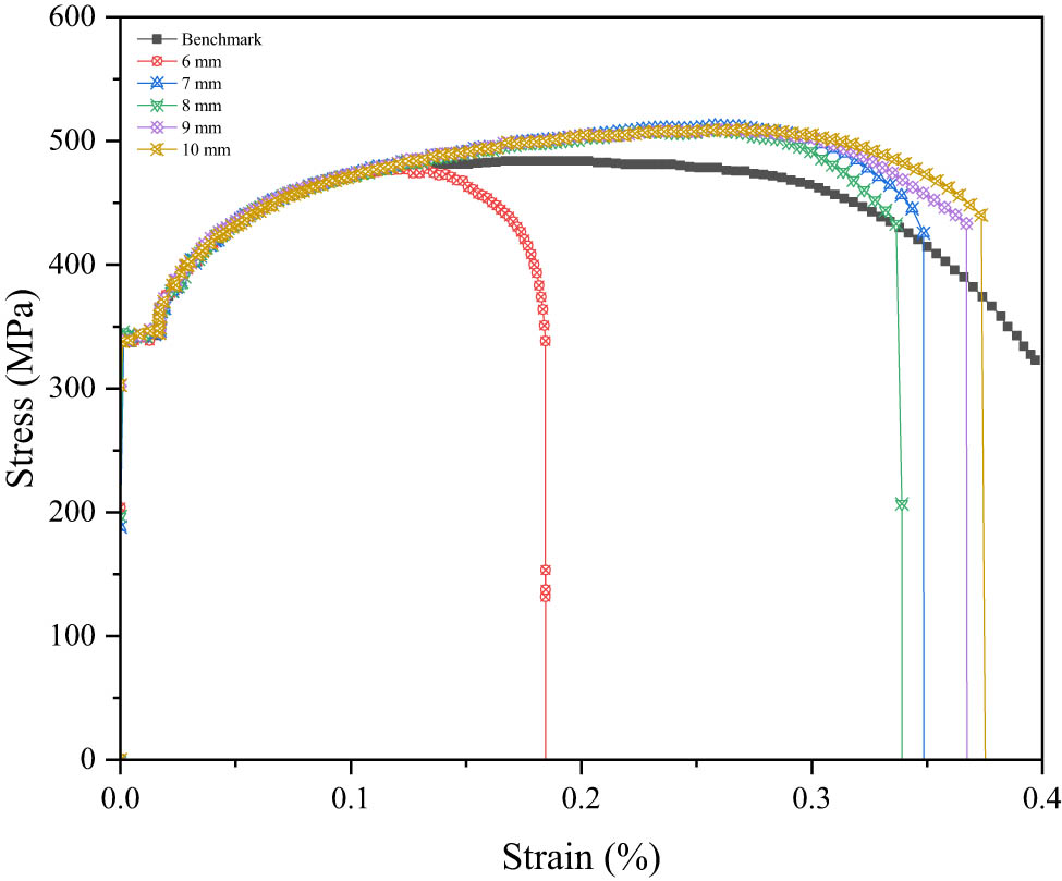
Stress–strain curve of mesh 6, 7, 8, 9, and 10 mm.
4 Research methodology
4.1 Laboratory experiment set-up
Cryogenic tensile testing experiments were previously conducted by Paik et al. with temperature variations of 20, −40, −80, −100, −130, and −160°C using AH32 material. However, the study only used specimens conforming to the ASTM E8/E8M Dog-bone standard, which is commonly used. Further research was conducted by Cerik et al. and Kõrgesaar et al., where the studies included several modifications and changes in geometry to create characterizations for each modified tensile specimen shape. The simulated specimens’ geometric variations will include shapes from Cerik et al. [41] in Figure 6a, such as Central Hole (CH), Notched Tensile (NT20), and Plane Strain Tension (PST). Additionally, shapes from Kõrgesaar et al. [42] Figure 6b shows several geometries that will be used, including Dog Bone (DB), CH, and Notched Tensile (NT). Several geometries, such as Central Hole and Central Hole, have similar geometries but different dimensions, which should be considered in the simulation. Similarly, PST and Notched Tensile are comparable in their geometric modifications.
![Figure 6
Geometry specimens: (a) designed based on Cerik et al. [41], and (b) designed based on Kõrgesaar et al. [42].](/document/doi/10.1515/jmbm-2024-0018/asset/graphic/j_jmbm-2024-0018_fig_006.jpg)
The test values were from Paik et al. [32]. The mechanical properties of the AH32 steel specimen (Table 2) were obtained from a series of tensile testing. Testing was conducted using a universal testing machine equipped with a cooling chamber to lower the temperature to a specified point, as shown in Figure 7a. Following the tests conducted by Paik, the acquired engineering stress–strain curve is illustrated in Figure 7b.
Mechanical properties of AH32 at various temperatures from tension tests done by Paik et al. [32]
| Property | 20°C | −40°C | −80°C | −100°C | −130°C | −160°C |
|---|---|---|---|---|---|---|
| Elastic modulus, E (GPa) | 205.8 | 205.8 | 205.8 | 205.8 | 205.8 | 205.8 |
| Yield strength, σ Y (MPa) | 358.03 | 391.02 | 433.48 | 472.52 | 546.74 | 672.96 |
| Ultimate tensile strength, σ T (MPa) | 497.07 | 537.81 | 579.13 | 605.10 | 652.28 | 739.36 |
| Ultimate tensile strain, ε τ | 0.193 | 0.207 | 0.222 | 0.223 | 0.211 | 0.163 |
| Fracture strain (−), ε f | 0.376 | 0.423 | 0.430 | 0.448 | 0.409 | 0.336 |
![Figure 7
Experimental setup and results [31]: (a) universal testing machine with cooling chamber, and (b) engineering stress–strain curve.](/document/doi/10.1515/jmbm-2024-0018/asset/graphic/j_jmbm-2024-0018_fig_007.jpg)
Experimental setup and results [31]: (a) universal testing machine with cooling chamber, and (b) engineering stress–strain curve.
4.2 Numerical configuration
This study utilizes ABAQUS FEA for nonlinear numerical analysis. The formulas in Eqs. (6) and (7) provide the algorithm used in this simulation testing [43].
In this algorithm, the acceleration at time t
where
Boundary conditions in this study are shown in Figure 8, where the nodal axial force is applied to both sides until the specimen fails. The axial nodal force values are chosen using a uniform load force on each side. Script “RP-1” indicates that the specimen will be pulled in the positive y-axis direction (right), while script “RP-2” will pull the specimen in the negative y-axis direction (left). The software performs the meshing process automatically using a 3 mm mesh. Additionally, the simulation is completed when the specimen fails, with a completion time of 1 × 10⁻⁴ s. This condition is applied to all specified variations. The output data, plotted on the x-axis and y-axis, will show the plastic strain and normal stress values.

Boundary condition of tensile test with ABAQUS Unified FEA.
Additionally, the material and specimen model settings can be configured in ABAQUS software using engineering data. The material model settings are briefly explained in Figure 9. Starting with the stress–strain curve from previous research, the geometry for testing is determined before specifying the mechanical parameters of the specimen. Parameters such as Young’s modulus, yield stress, ultimate strength, and others are defined. After converting the engineering stress–strain curve to a true stress–strain curve, this can be entered into the plasticity table (multilinear isotropic hardening). This process is repeated for the various temperatures and geometries specified.

Flowchart for the FE methodology for the current work.
5 Results and discussion
5.1 Effect of the designed specimen geometry
Further studies were conducted using ABAQUS simulations with the same material but with different temperature variations and geometries to determine each specimen’s characteristics. The designed temperatures used were 20, −40, −80, −100, −130, and −160°C. Additionally, various designed geometries were also used to investigate their characteristics, including CH, Notched Tension (NT20), PST, DB, and Notched Tensile (NT). The FE simulation results are summarized in Tables 3–6.
Post-mortem necking images from testing at 20°C
| Designed specimen based on [41] – 20°C | Designed specimen based on [42] – 20°C |
|---|---|
 |
 |
 |
 |
 |
 |
Post-mortem failure images from testing at 20°C
| Designed specimen based on [41] – 20°C | Designed specimen based on [42] – 20°C |
|---|---|
 |
 |
 |
 |
 |
 |
Post-mortem necking images from testing at −40°C
| Designed specimen based on [41] – minus 40°C | Designed specimen based on [42] – minus 40 °C |
|---|---|
 |
 |
 |
 |
 |
 |
Post-mortem failure images from testing at −40°C
| Designed specimen based on [41] – minus 40°C | Designed specimen based on [42] – minus 40°C |
|---|---|
 |
 |
 |
 |
 |
 |
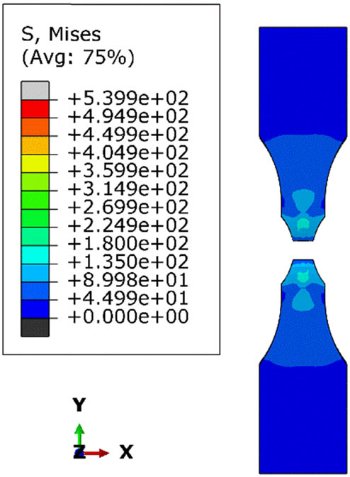
During necking at temperatures of 20 and −40°C, the CH specimen exhibited similar contours in terms of stress distribution and the forces affecting each specimen. However, the values differed for each contour; at 20°C, the red contour had a value of 4.565 × 10², while at −40°C, it had a value of 4.945 × 10². This indicates that lower temperatures result in higher stress values. At the point of failure, the same specimen showed similar contour values with some differences, but the resulting fractures were identical. Therefore, it can be concluded that temperature in this simulation only affects the hardness of the specimen or the stress and force it experiences. In notched tension test specimens at 20 and −40°C, the stress distribution during necking at 20°C shows a uniform spread in the neck area with the highest stress value of 4.980 × 10². At failure, the maximum stress is distributed over a wider area around the neck with the same value, indicating that the material at this temperature can withstand high stress before failing. At −40°C, the stress distribution during necking is similar to that at 20°C but with a higher stress value of 5.399 × 10², showing higher stress concentration in the neck area. At failure, the stress distribution is similar to that at 20°C but with a higher maximum stress value, indicating that the material at lower temperatures is stiffer and more resistant to plastic deformation before failing.
In-plane strain tension test specimens at 20 and −40°C, the stress distribution during necking at 20°C shows a uniform spread in the neck area, with the highest stress value being 4.805 × 10². Upon failure, the maximum stress extends over a broader area around the neck, maintaining the same value, indicating the material’s ability to withstand high stress before failure at this temperature. At −40°C, the stress distribution during necking is similar to that at 20°C but with a higher stress value of 5.395 × 10², indicating a higher stress concentration in the neck area. At failure, the stress distribution remains similar to that at 20°C but with a higher maximum stress value, suggesting that the material is stiffer and more resistant to plastic deformation at lower temperatures.
In DB specimens tested at 20°C, the stress distribution during necking displays a uniform spread in the neck area, with the peak stress reaching 4.980 × 10². At failure, the maximum stress extends over a broader region around the neck while maintaining the same value, indicating that the material can endure high-stress levels before breaking at this temperature. For the specimens tested at −40°C, the stress distribution during necking shows a similar pattern to that at 20°C but with a higher peak stress value of 5.395 × 10², indicating increased stress concentration in the neck region. During failure, the stress distribution remains similar to that at 20°C but with a higher maximum stress value, suggesting that the material at lower temperatures is stiffer and more resistant to plastic deformation before failure.
For the CH specimens tested at 20°C, the stress distribution during necking shows a uniform spread in the neck area, with the highest stress value reaching 4.980 × 10². When failure occurs, the maximum stress extends across a broader region around the neck, maintaining the same value, indicating that the material at this temperature can withstand high-stress levels before failing. In contrast, for the specimens tested at −40°C, the stress distribution during necking is similar to that at 20°C. Still, it exhibits a higher peak stress value of 5.395 × 10², suggesting an increased stress concentration in the neck area. At the point of failure, the stress distribution remains similar to that at 20°C but with a higher maximum stress value, implying that the material at lower temperatures is stiffer and more resistant to plastic deformation before breaking.
For the Notched Tensile specimens at 20°C, the stress distribution during necking shows a uniform spread in the neck area with the highest stress value of 4.980 × 10². At failure, the maximum stress is distributed over a broader region around the neck while maintaining the same value, indicating that the material at this temperature can withstand high-stress levels before failing. In contrast, for the specimens tested at −40°C, the stress distribution during necking is similar to that at 20°C. Still, it exhibits a higher peak stress value of 5.395 × 10², suggesting an increased stress concentration in the neck area. At failure, the stress distribution remains similar to that at 20°C but with a higher maximum stress value, implying that the material at lower temperatures is stiffer and more resistant to plastic deformation before breaking.
5.2 Effect of the selected low-temperature conditions
Figure 10(a) displays the stress–strain curves for three different geometries (CH, NT20, and PST) tested at 20°C. The CH specimen shows a gradual increase in stress up to a peak value of approximately 600 MPa, followed by a gradual decrease, indicating ductile behavior with significant necking and strain hardening and a total strain before failure around 0.25, demonstrating high ductility. The NT20 specimen reaches a peak stress of approximately 500 MPa, with a more pronounced drop after the peak stress, indicating less ductility than the CH specimen and a total strain before failure around 0.15, suggesting moderate ductility. The PST specimen shows a peak stress of approximately 650 MPa, the highest among the three geometries, with a sharp drop after the peak stress, indicating brittle behavior and a total strain before failure around 0.10, showing the least ductility.

Comparison of stress–strain curves from designed geometry results of CH, Notched Tension (NT20), PST, DB, Notched Tensile (NT): (a) at 20°C, (b) at −40°C, (c) at −80°C, and (d) at −160°C.
Figure 10(b) presents the stress–strain curves for the same geometries tested at −40°C. The CH specimen shows a peak stress of approximately 650 MPa, with a more abrupt drop after the peak stress than the 20°C test, suggesting reduced ductility and a total strain before failure around 0.20, indicating less ductility. The NT20 specimen reaches a peak stress of approximately 550 MPa, with a significant drop after the peak stress similar to the behavior at 20°C but more pronounced, indicating lower ductility and a total strain before failure around 0.12, less than at 20°C, suggesting reduced ductility at lower temperatures. The PST specimen exhibits a peak stress of approximately 700 MPa, the highest among the three geometries, with a sharp drop after the peak stress indicating brittle behavior, similar to the test at 20°C but more severe, and a total strain before failure around 0.08, showing the least ductility and indicating that lower temperatures significantly reduce the material’s ability to deform plastically.
Figure 10(c) presents the stress–strain curves for three different geometries (CH, DB, and NT) tested at 20°C. The CH specimen exhibits a gradual increase in stress, reaching a peak value of approximately 550 MPa. There is a gradual decline after reaching the peak stress, indicating ductile behavior with significant necking and strain hardening. The total strain before failure is around 0.25, demonstrating high ductility. The DB specimen shows a peak stress of approximately 450 MPa. The stress–strain curve reveals a steady decrease after the peak stress, indicating moderate ductility and the total strain before failure is around 0.30, which is higher than the CH specimen, suggesting more excellent ductility. The NT (Notched Tension) specimen reaches a peak stress of approximately 600 MPa, the highest among the three geometries. The stress–strain curve exhibits a sharp drop after the peak stress, indicating brittle behavior, with the total strain before failure around 0.10, indicating the least ductility among the three geometries.
Figure 10(d) shows the stress–strain curves for the same three geometries tested at −40°C. The CH specimen shows a peak stress of approximately 650 MPa. The stress–strain curve indicates a more abrupt decline after the peak stress than the 20°C test, suggesting reduced ductility and the total strain before failure is around 0.35, higher than at 20°C, indicating better ductility at lower temperatures. The DB specimen reaches a peak stress of approximately 550 MPa. The curve shows a significant drop after the peak stress, similar to the behavior at 20°C but more pronounced, indicating lower ductility. The total strain before failure is around 0.25, less than at 20°C, suggesting reduced ductility at lower temperatures. The NT (Notched Tension) specimen exhibits a peak stress of approximately 700 MPa, the highest among the three geometries. The stress–strain curve shows a sharp drop after the peak stress, indicating brittle behavior, similar to the test at 20°C but more severe. The total strain before failure is around 0.15, showing the least ductility and indicating that lower temperatures significantly reduce the material’s ability to deform plastically. In summary, PST and NT specimens exhibit the highest peak stress values at both temperatures, indicating the strongest but most brittle behavior. CH specimens demonstrate the highest ductility with a higher total strain before failure but lower peak stress than PST and NT. Lower temperatures (−40°C) increase the peak stress values for all geometries but significantly reduce their ductility, leading to more brittle failure modes. NT20 and DB specimens exhibit intermediate behavior, with moderate peak stress and ductility, but show a more pronounced drop in stress after reaching the peak, especially at lower temperatures.
The temperature variations in material behavior based on the stress–strain curves for designed geometries were tested at various temperatures: 20, −40, −80, and −160°C. This analysis aims to understand how temperature affects the strength and ductility of the material, as well as to identify the failure characteristics occurring at each temperature variation. In Figure 11(a), designed geometry at 20°C, the CH specimen exhibits high ductility with a peak stress of approximately 600 MPa and a gradual decline. The NT20 (Notched Tension at 20°C) specimen shows moderate ductility with a peak stress around 500 MPa and a pronounced drop after the peak. The PST specimen demonstrates the highest peak stress at around 650 MPa but with a sharp decline, indicating more brittle behavior. In Figure 11(b), designed geometry at −40°C, the CH specimen displays reduced ductility with peak stress of approximately 650 MPa and a more abrupt decline. In contrast, the NT20 specimen indicates lower ductility with a peak stress around 550 MPa and a significant drop after the peak. The PST specimen again shows the highest peak stress, approximately 700 MPa, with a sharp decline, indicating brittle behavior. In Figure 11(c), designed geometry at −80°C, the DB specimen demonstrates moderate ductility with a peak stress around 700 MPa and a steady decline. In contrast, the NT (Notched Tension) specimen exhibits brittle behavior with a peak stress of around 600 MPa and a sharp drop. The CH specimen shows high ductility with a gradual decline after reaching a peak stress of around 650 MPa. In Figure 11(d), designed geometry at −160°C, the DB specimen indicates reduced ductility with a peak stress of around 650 MPa and a significant drop. In contrast, the CH specimen exhibits high ductility with a peak stress around 700 MPa and a gradual decline. The NT specimen shows a peak stress of around 600 MPa with a sharp decline, indicating very brittle behavior at this low temperature.

Comparison of stress–strain curves from designed temperature results of CH, Notched Tension (NT20), PST, DB, Notched Tensile (NT): (a) at 20°C, (b) at −40°C, (c) at −80°C, and (d) at −160°C.
Therefore, across all temperatures, lower temperatures (−40, −80, and −160°C) generally increase peak stress values but significantly reduce ductility, leading to more brittle failure modes. CH Specimens typically demonstrate higher ductility with gradual stress declines, while NT and DB specimens show higher peak stresses with more pronounced drops, indicating more brittle behavior at lower temperatures. The current methodology may be extended to investigate critical materials, which may be used in renewable energy harvest infrastructure, such as photovoltaic [45,46,47,48,49,50,51], and in advanced material development, e.g., optic, composite, and polymer testing [52,53,54,55,56,57]. Optimization and decision-making can be considered to be deployed to select the best according to the main criteria (e.g., durability, crashworthiness, lifetime, etc.) of several proposed material configurations so that the findings can be implemented in real-world case applications [58,59,60,61].
6 Conclusions
This study investigated the behavior of AH32 steel and other materials at cryogenic temperatures for ship hull applications, combining experimental testing and ABAQUS Unified FEA simulations. Key findings include increased yield stress and ultimate tensile strength for AH32 steel at lower temperatures but with a notable reduction in ductility, raising concerns about brittle fracture. ABAQUS simulations effectively replicated experimental conditions, underscoring the importance of selecting appropriate mesh sizes for accuracy.
Geometrical variations provided critical insights: central hole specimens exhibited significant stress concentration and higher crack initiation risk, notched tensile specimens showed a pronounced reduction in fracture toughness, and plane strain tension specimens offered insights into uniform stress distribution. Standard dog-bone specimens confirmed trends of increased strength and reduced ductility at lower temperatures. These findings highlight the need for careful material selection and design strategies to mitigate brittle fracture risks in Arctic conditions.
Overall, this study advances the understanding of material behavior at cryogenic temperatures, providing valuable information for marine structures’ design and safety standards. Future research should explore additional materials and advanced simulation techniques to enhance the resilience and performance of structures in extreme environments.
Acknowledgments
This work's analysis was also completed by the collaborations between Universitas Sebelas Maret (UNS) and the National Research and Innovation Agency (BRIN) under Cooperation Agreement Contract Number 179/V/KS/06/2024 from BRIN and 541/UN27.08.1/HK.07.00/2024 from UNS. The authors are grateful for the reviewer's valuable comments, which improved the manuscript.
-
Funding information: The publication funding of this article is supported by internal funding of Universitas Sebelas Maret (UNS).
-
Author contributions: All authors have accepted responsibility for the entire content of this manuscript and consented to its submission to the journal reviewed all the results and approved the final version of the manuscript. MFAA: Formal analysis, Writing – Original Draft, Writing – Review & Editing; SS: Formal analysis, Investigation, Writing – Original Draft; ARP: Methodology, Writing – Original Draft, Writing – Review – Editing, Supervision, Funding acquisition; TM: Methodology, Software, Supervision, Resources; QTD: Conceptualization, Methodology; BS: Writing – Review & Editing, Visualization; FBL: Methodology, Funding acquisition; HN: Data Curation, Visualization.
-
Conflict of interest: The authors state no conflict of interest.
-
Data availability statement: The authors declare that the data supporting the findings of this study are available within the article.
References
[1] Tseng PH, Cullinane K. Key criteria influencing the choice of Arctic shipping: a fuzzy analytic hierarchy process model. Mar Pol Manag. 2018;45:422–38. 10.1080/03088839.2018.1443225.Suche in Google Scholar
[2] Noh Y, Kim J, Kim J, Chang D. Economic evaluation of BOG management systems with LNG cold energy recovery in LNG import terminals considering quantitative assessment of equipment failures. Appl Therm Eng. 2018;143:1034–45. 10.1016/j.applthermaleng.2018.08.029.Suche in Google Scholar
[3] Chaebi H, Namin AS, Rostamzadeh H. Exergoeconomic optimization of a novel cascade Kalina/Kalina cycle using geothermal heat source and LNG cold energy recovery. J Clean Prod. 2018;189:279–96. 10.1016/j.jclepro.2018.04.049.Suche in Google Scholar
[4] Ma G, Lu H, Cui G, Huang K. Multi-stage Rankine cycle (MSRC) model for LNG cold-energy power generation system. Energy. 2018;165:673–88. 10.1016/j.energy.2018.09.203.Suche in Google Scholar
[5] Gritsenko D. Explaining choices in energy infrastructure development as a network of adjacent action situations: The case of LNG in the Baltic Sea region. Energy Pol. 2018;112:74–83. 10.1016/j.enpol.2017.10.014.Suche in Google Scholar
[6] Gunnarsson B. Recent ship traffic and developing shipping trends on the Northern Sea Route—Policy implications for future arctic shipping. Mar Pol. 2021;124:104369. 10.1016/j.marpol.2020.104369.Suche in Google Scholar
[7] Pospíšil J, Charvát P, Arsenyeva O, Klimeš L, Špiláček M, Klemeš JJ. Energy demand of liquefaction and regasification of natural gas and the potential of LNG for operative thermal energy storage. Renew Sustain Energy Rev. 2019;99:1–15. 10.1016/j.rser.2018.09.027.Suche in Google Scholar
[8] Lu H, Guo L, Azimi M, Huang K. Oil and Gas 4.0 era: A systematic review and outlook. Comput Ind. 2019;111:68–90. 10.1016/j.compind.2019.06.007.Suche in Google Scholar
[9] Wang K, Qian X, He Y, Shi T, Zhang X. Failure analysis integrated with prediction model for LNG transport trailer and thermal hazards induced by an accidental VCE: A case study. Eng Fail Anal. 2020;108:104350. 10.1016/j.engfailanal.2019.104350.Suche in Google Scholar
[10] Zhang J, Meerman H, Benders R, Faaij A. Comprehensive review of current natural gas liquefaction processes on technical and economic performance. Appl Therm Eng. 2020;166:114736. 10.1016/j.applthermaleng.2019.114736.Suche in Google Scholar
[11] Yang JH, Yoon Y, Ryu M, An SK, Shin J, Lee CJ. Integrated hydrogen liquefaction process with steam methane reforming by using liquefied natural gas cooling system. Appl Energy. 2019;255:113840. 10.1016/j.apenergy.2019.113840.Suche in Google Scholar
[12] Wang Q, Song Q, Zhang J, Liu R, Zhang S, Chen G. Experimental studies on a natural gas liquefaction process operating with mixed refrigerants and a rectifying column. Cryogenic. 2019;99:7–17. 10.1016/j.cryogenics.2019.02.007.Suche in Google Scholar
[13] Botão RP, Costa HK, Santos EM. Global Gas and LNG markets: Demand, supply dynamics, and implications for the future. Energy. 2023;16:5223. 10.3390/en16135223.Suche in Google Scholar
[14] Lee K, Murakami S, Ölҫer AI, Dong T, Estebanez G, Schönborn A. Hydrogen enriched LNG fuel for maritime applications – A life cycle study. Int J Hydrogen Energy. 2024;78:333–43. 10.1016/j.ijhydene.2024.06.273.Suche in Google Scholar
[15] Li T, He X, Gao P. Analysis of offshore LNG storage and transportation technologies based on patent informatics. Clean Eng Technol. 2021;5:100317. 10.1016/j.clet.2021.100317.Suche in Google Scholar
[16] Aneziris O, Gerbec M, Koromila I, Nivolianitou Z, Pilo F, Salzano E. Safety guidelines and a training framework for LNG storage and bunkering at ports. Saf Sci. 2021;138:105212. 10.1016/j.ssci.2021.105212.Suche in Google Scholar
[17] Peng Y, Zhao X, Zuo T, Wang W, Song X. A systematic literature review on port LNG bunkering station. Transp Res D: Transp Environ. 2021;91:102704. 10.1016/j.trd.2021.102704.Suche in Google Scholar
[18] IGLNGI. Benefits of LNG. Neuilly-sur-Seine: International Group of Liquefied Natural Gas Importers; 2024.Suche in Google Scholar
[19] IEF. LNG: A versatile energy source comes into its own. Riyadh: International Energy Forum; 2023.Suche in Google Scholar
[20] Zou Q, Yi C, Wang K, Yin X, Zhang Y. Global LNG market: Supply-demand and economic analysis. IOP Conf Ser Earth Environ Sci. 2022;983:012051. 10.1088/1755-1315/983/1/012051.Suche in Google Scholar
[21] Lakhal SY. A study on the maritime transport network design under different charter rates: The case of LNG transport between Qatar & Turkey. Oper Suppl Chain Manag. 2018;11:13–25. 10.31387/oscm0300196.Suche in Google Scholar
[22] Meza A, Ari I, Sada MA, Koç M. Disruption of maritime trade chokepoints and the global LNG trade: An agent-based modeling approach. Mar Transp Res. 2022;3:100071. 10.1016/j.martra.2022.100071.Suche in Google Scholar
[23] Wu D, Wang N, Yu A, Wu N. Vulnerability analysis of global container shipping liner network based on main channel disruption. Mar Pol Manag. 2019;46(4):394–409. 10.1080/03088839.2019.1571643.Suche in Google Scholar
[24] Bae DM, Prabowo AR, Cao B, Sohn JM, Zakki AF, Wang Q. Numerical simulation for the collision between side structure and level ice in event of side impact scenario. Lat Am J Solid Struct. 2016;13:2691–704. 10.1590/1679-78252975.Suche in Google Scholar
[25] Cao B, Bae DM, Sohn JM, Prabowo AR, Chen TH, Li H. Numerical analysis for damage characteristics caused by ice collision on side structure. Proc Int Conf Offshore Mech Arct Eng. 2016;8:V008T07A019. 10.1115/OMAE2016-54727.Suche in Google Scholar
[26] Pruyn JFJ. Will the Northern Sea Route ever be a viable alternative? Mar Pol Manag. 2016;43:661–75. 10.1080/03088839.2015.1131864.Suche in Google Scholar
[27] Prabowo AR, Tuswan T, Ridwan R. Advanced development of sensors’ roles in maritime‐based industry and research: From field monitoring to high‐risk phenomenon measurement. Appl Sci. 2021;11:3954. 10.3390/app11093954.Suche in Google Scholar
[28] Prabowo AR, Sohn JM, Byeon JH, Bae DM, Zakki AF, Cao B. Structural analysis for estimating damage behavior of double hull under ice-grounding scenario models. Key Eng Mat. 2017;754:303–6. 10.4028/www.scientific.net/KEM.754.303.Suche in Google Scholar
[29] Prabowo AR, Bahatmaka A, Cho JH, Sohn JM, Bae DM, Samuel S, et al. Analysis of structural crashworthiness on a non-ice class tanker during stranding accounting for the sailing routes. Marit Transp Harvest Sea Res. 2016;1:645–54.Suche in Google Scholar
[30] Prabowo AR, Byeon JH, Cho HJ, Sohn JM, Bae DM, Cho JH. Impact phenomena assessment: Part I-Structural performance of a tanker subjected to ship grounding at the Arctic. MATEC Web Conf. 2018;159:02061. 10.1051/matecconf/201815902061.Suche in Google Scholar
[31] Shu Y, Zhu Y, Xu F, Gan L, Lee PTW, Yin J, et al. Path planning for ships assisted by the icebreaker in ice-covered waters in the Northern Sea Route based on optimal control. Ocean Eng. 2023;267:113182. 10.1016/j.oceaneng.2022.113182.Suche in Google Scholar
[32] Paik JK, Lee DH, Park DK, Ringsberg JW. Full-scale collapse testing of a steel stiffened plate structure under axial-compressive loading at a temperature of −80°C. Ship Offshore Struct. 2021;16:255–70. 10.1080/17445302.2020.1791685.Suche in Google Scholar
[33] Nubli H, Suryanto S, Fajri A, Sohn JM, Prabowo AR. A review on the hull structural steels for ships carrying liquefied gas: Materials performance subjected to low temperatures. Proc Struct Integr. 2023;48:73–80. 10.1016/j.prostr.2023.07.112.Suche in Google Scholar
[34] Barat K, Bar HN, Mandal D, Roy H, Sivaprasad S, Tarafder S. Low temperature tensile deformation and acoustic emission signal characteristics of AISI 304LN stainless steel. Mat Sci Eng A. 2014;597:37–45. 10.1016/j.msea.2013.12.067.Suche in Google Scholar
[35] Yan JB, Kong G, Zhang L. Low-temperature tensile behaviours of 6061-T6 aluminium alloy: Tests, analysis, and numerical simulation. Structures. 2023;56:105054. 10.1016/j.istruc.2023.105054.Suche in Google Scholar
[36] Callister WD. Materials science and engineering: An introduction. 8th edn. New Jersey: Wiley; 2019.Suche in Google Scholar
[37] Hibbeler RC. Mechanics of materials. 9th edn.. New Jersey: Pearson Prentice Hall; 2013.Suche in Google Scholar
[38] Suryanto S, Prabowo AR, Muttaqie T, Istanto I, Adiputra R, Muhayat N, et al. Evaluation of high-tensile steel using nonlinear analysis: Experiment-FE materials benchmarking of LNG carrier structures under low-temperature conditions. Energy Rep. 2023;9:149–61. 10.1016/j.egyr.2023.05.252.Suche in Google Scholar
[39] ASTM. ASTM E8/E8M-16a - Standard test methods for tension testing of metallic materials. Pennsylvania: ASTM International; 2016.Suche in Google Scholar
[40] Dieter GE. Mechanical metallurgy. 3rd edn.. New Jersey: McGraw-Hill; 1961.10.5962/bhl.title.35895Suche in Google Scholar
[41] Cerik BC, Park B, Park SJ, Choung J. Modeling, testing and calibration of ductile crack formation in grade DH36 ship plates. Mar Struct. 2019;66:27–43. 10.1016/j.marstruc.2019.03.003.Suche in Google Scholar
[42] Kõrgesaar M, Romanoff J, Remes H, Palokangas P. Experimental and numerical penetration response of laser-welded stiffened panels. Int J Impact Eng. 2018;114:78–92. 10.1016/j.ijimpeng.2017.12.014.Suche in Google Scholar
[43] Prabowo AR, Bae DM, Sohn JM, Zakki AF. Evaluating the parameter influence in the event of a ship collision based on the finite element method approach. Int J Technol. 2016;7:253–72. 10.14716/ijtech.v7i4.2104.Suche in Google Scholar
[44] Prabowo AR, Muttaqie T, Sohn JM, Bae DM. Nonlinear analysis of inter-island roro under impact: Effects of selected collision’s parameters on the crashworthy double-side structures. J Braz Soc Mech Sci Eng. 2018;40:248. 10.1007/s40430-018-1169-6.Suche in Google Scholar
[45] Rasheed M, Shihab S, Alabdali O, Hassan HH. Parameters extraction of a single-diode model of photovoltaic cell using false position iterative method. J Phy Conf Ser. 2021;1879:032113. 10.1088/1742-6596/1879/3/032113.Suche in Google Scholar
[46] Rasheed M, Shihab S, Mohammed OY, Al-Adili A. Parameters estimation of photovoltaic model using nonlinear algorithms. J Phy Conf Ser. 2021;1795:012058. 10.1088/1742-6596/1795/1/012058.Suche in Google Scholar
[47] Bouras D, Fellah M, Mecif A, Barillé R, Obrosov A, Rasheed M. High photocatalytic capacity of porous ceramic-based powder doped with MgO. J Korean Ceram Soc. 2023;60(1):155–68. 10.1007/s43207-022-00254-5.Suche in Google Scholar
[48] Sarhan MA, Shihab S, Kashem BE, Rasheed M. New exact operational shifted pell matrices and their application in astrophysics. J Phys Conf Ser. 2021;1879:022122. 10.1088/1742-6596/1879/2/022122.Suche in Google Scholar
[49] Shihab S, Rasheed M, Alabdali O, Abdulrahman AA. A novel predictor-corrector hally technique for determining the parameters for nonlinear solar cell equation. J Phys Conf Ser. 2021;1879:022120. 10.1088/1742-6596/1879/2/022120.Suche in Google Scholar
[50] Rasheed M, Al-Darraji MN, Shihab S, Rashid A, Rashid T. Solar PV modelling and parameter extraction using iterative algorithms. J Phys Conf Ser. 2021;1963:012059. 10.1088/1742-6596/1963/1/012059.Suche in Google Scholar
[51] Prasetyo SD, Arifin Z, Prabowo AR, Budiana EP. Investigation of the addition of fins in the collector of water/Al2O3-based PV/T system: Validation of 3D CFD with experimental study. Case Stud Therm Eng. 2024;60:104682. 10.1016/j.csite.2024.104682.Suche in Google Scholar
[52] Bouras D, Rasheed M, Barille R, Aldaraji MN. Efficiency of adding DD3 + (Li/Mg) composite to plants and their fibers during the process of filtering solutions of toxic organic dyes. Opt Mater. 2022;131:112725. 10.1016/j.optmat.2022.112725.Suche in Google Scholar
[53] Naufal AM, Prabowo AR, Muttaqie T, Hidayat A, Purwono J, Adiputra R, et al. Characterization of sandwich materials – Nomex-Aramid carbon fiber performances under mechanical loadings: Nonlinear FE and convergence studies. Rev Adv Mat Sci. 2024;63:20230177. 10.1515/rams-2023-0177.10.1515/rams-2023-0177Suche in Google Scholar
[54] Smaradhana DF, Prabowo AR, Ganda ANF. Exploring the potential of graphene materials in marine and shipping industries – A technical review for prospective application on ship operation and material-structure aspects. J Ocean Eng Sci. 2021;6(3):299–316. 10.1016/j.joes.2021.02.004.10.1016/j.joes.2021.02.004Suche in Google Scholar
[55] Naufal AM, Prabowo AR, Muttaqie T, Hidayat A, Adiputra R, Muhayat N, et al. Three-point bending assessment of cold water pipe (CWP) sandwich material for ocean thermal energy conversion (OTEC). Proc Struct Integr. 2023;47:133–41. 10.1016/j.prostr.2023.07.004.Suche in Google Scholar
[56] Sakuri S, Surojo E, Ariawan D, Prabowo AR. Experimental investigation on mechanical characteristics of composite reinforced cantala fiber (CF) subjected to microcrystalline cellulose and fumigation treatments. Compos Commun. 2020;21:100419. 10.1016/j.coco.2020.100419.Suche in Google Scholar
[57] Akbar HI, Surojo E, Ariawan D, Prabowo AR. Experimental study of quenching agents on Al6061–Al2O3 composite: Effects of quenching treatment to microstructure and hardness characteristics. Res Eng. 2020;6:100105. 10.1016/j.rineng.2020.100105.Suche in Google Scholar
[58] Alabdali O, Shihab S, Rasheed M, Rashid T. Orthogonal Boubaker-Turki polynomials algorithm for problems arising in engineering. AIP Conf Proc. 2022;2386:050019. 10.1063/5.0066860.Suche in Google Scholar
[59] Rahmaji T, Prabowo AR, Tuswan T, Muttaqie T, Muhayat N, Baek SJ. Design of fast patrol boat for improving resistance, stability, and seakeeping performance. Designs. 2022;6(6):105. 10.3390/designs6060105.Suche in Google Scholar
[60] Nubli H, Sohn JM, Prabowo AR. Layout optimization for safety evaluation on LNG-fueled ship under an accidental fuel release using mixed-integer nonlinear programming. Int J Nav Arch Ocean Eng. 2022;14:100443. 10.1016/j.ijnaoe.2022.100443.Suche in Google Scholar
[61] Diatmaja H, Prabowo AR, Adiputra R, Muhayat N, Baek SJ, Huda N, et al. Comparative evaluation of design variations in prototype fast boats: A hydrodynamic characteristic-based approach. Math Model Eng Prob. 2023;10(5):1487–507. 10.18280/mmep.100501.Suche in Google Scholar
© 2024 the author(s), published by De Gruyter
This work is licensed under the Creative Commons Attribution 4.0 International License.
Artikel in diesem Heft
- Research Articles
- Evaluation of the mechanical and dynamic properties of scrimber wood produced from date palm fronds
- Performance of doubly reinforced concrete beams with GFRP bars
- Mechanical properties and microstructure of roller compacted concrete incorporating brick powder, glass powder, and steel slag
- Evaluating deformation in FRP boat: Effects of manufacturing parameters and working conditions
- Mechanical characteristics of structural concrete using building rubbles as recycled coarse aggregate
- Structural behavior of one-way slabs reinforced by a combination of GFRP and steel bars: An experimental and numerical investigation
- Effect of alkaline treatment on mechanical properties of composites between vetiver fibers and epoxy resin
- Development of a small-punch-fatigue test method to evaluate fatigue strength and fatigue crack propagation
- Parameter optimization of anisotropic polarization in magnetorheological elastomers for enhanced impact absorption capability using the Taguchi method
- Determination of soil–water characteristic curves by using a polymer tensiometer
- Optimization of mechanical characteristics of cement mortar incorporating hybrid nano-sustainable powders
- Energy performance of metallic tubular systems under reverse complex loading paths
- Enhancing the machining productivity in PMEDM for titanium alloy with low-frequency vibrations associated with the workpiece
- Long-term viscoelastic behavior and evolution of the Schapery model for mirror epoxy
- Laboratory experimental of ballast–bituminous–latex–roving (Ballbilar) layer for conventional rail track structure
- Eco-friendly mechanical performance of date palm Khestawi-type fiber-reinforced polypropylene composites
- Isothermal aging effect on SAC interconnects of various Ag contents: Nonlinear simulations
- Sustainable and environmentally friendly composites: Development of walnut shell powder-reinforced polypropylene composites for potential automotive applications
- Mechanical behavior of designed AH32 steel specimens under tensile loading at low temperatures: Strength and failure assessments based on experimentally verified FE modeling and analysis
- Review Article
- Review of modeling schemes and machine learning algorithms for fluid rheological behavior analysis
- Special Issue on Deformation and Fracture of Advanced High Temperature Materials - Part I
- Creep–fatigue damage assessment in high-temperature piping system under bending and torsional moments using wireless MEMS-type gyro sensor
- Multiaxial creep deformation investigation of miniature cruciform specimen for type 304 stainless steel at 923 K using non-contact displacement-measuring method
- Special Issue on Advances in Processing, Characterization and Sustainability of Modern Materials - Part I
- Sustainable concrete production: Partial aggregate replacement with electric arc furnace slag
- Exploring the mechanical and thermal properties of rubber-based nanocomposite: A comprehensive review
- Experimental investigation of flexural strength and plane strain fracture toughness of carbon/silk fabric epoxy hybrid composites
- Functionally graded materials of SS316L and IN625 manufactured by direct metal deposition
- Experimental and numerical investigations on tensile properties of carbon fibre-reinforced plastic and self-reinforced polypropylene composites
- Influence of plasma nitriding on surface layer of M50NiL steel for bearing applications