The Relationship Between Stock Performance and Money Supply Based on VAR Model in the Context of E-commerce
-
Lianshi Qiu


Abstract
With the development of network technology, electronic money as a payment and settlement tool based on the network has been developing at an unprecedented speed. Based on the background of e-commerce, this study uses the data from June 2012 to June 2022 to establish a vector autoregressive model to study the interaction between oil prices, stock performance, and money supply. Such a model can not only further our understanding of the complex relationship between these important variables but also shed light on future oil prices. Granger causality test, impulse response function analysis, and variance decomposition analysis have been applied to variables in the model. The main finding is that oil price responds to changes in stock performance and money supply, stock performance is affected by both oil price and money supply, and changes in money supply can be explained by stock performance fluctuations. Such a relationship can help inform traders in e-commerce and investment banking to generate better predictions of future oil prices.
1 Introduction
Given its role as an indispensable raw industrial material, oil is a valuable commodity in the international economy, and oil price fluctuations can have a profound impact on economic performance of global economy. In many cases, oil supply shocks negatively affected global economy, resulting in higher inflation and lower economic growth. Therefore, establishing models that investigate the relationship between oil price and other economic variables can facilitate economists to implement effective fiscal and monetary policies that can mitigate the economic fluctuations stemming out from oil price changes. Moreover, investors can profit financially from correctly predicting the rise or fall in oil prices, providing incentives to research into this area. For these reasons, the relationship between oil price and other macroeconomic variables has been the topic of myriads of academic and corporate research for decades. With the development of network technology, it would also be meaningful to investigate such relationship in the context of e-commerce since it is a relatively new means of transaction. The higher efficiency of transactions conducted in e-commerce makes it even more important to generate reliable predictions of future oil prices to avoid potential losses because gains and losses can happen in a relatively shorter time frame.
This research aims to utilize the latest data collected between June 2012 and June 2022 to establish a vector autoregression (VAR) model with three lags that investigate the interactive relationship between oil prices, stock market performance, and money supply in the United States. The period June 2012–June 2022 is selected because past research that utilizes relatively outdated data may fail to reflect current changes in the relationship between oil price, stock market performance, and money supply. The escalation of Russo-Ukrainian war starting from 24 February 2022, in particular, is a crisis that caused severe disruption to global energy market and economy. The soaring energy prices adversely affected global supply chain, resulting in soaring inflation and constraining economic recovery from COVID-19 pandemic recession (Korosteleva, 2022). Therefore, it would be meaningful to construct a VAR model that examines the interactive relationship between oil price, stock market, and money supply under current circumstances. Such a model could not only further our understanding of the complex relationship between these important variables but also shed light on future oil prices. Granger causality test, impulse response function (IRF) analysis, and variance decomposition analysis have been applied to variables in the model. The main finding is that oil price responds to changes in stock performance and money supply, stock performance is affected by both oil price and money supply, and changes in money supply can be explained by stock performance fluctuations. This research is organized by the following structure: first, by reviewing existing literature, this article analyzes the theoretical mechanism of the research. Then, a VAR model that examines the interactive relationship between oil price, stock performance, and money supply under current circumstances is constructed. Finally, empirical analysis is conducted on the VAR model using the Granger causality test, IRF analysis, and variance decomposition analysis to derive further implications regarding the interactions between the variables.
2 Literature Review
The economic impact of oil prices has been studied in various research focusing on different countries and time periods. Much established research is dedicated to the relationship between oil price and macroeconomic indicators, including real gross domestic product (GDP) growth rate, inflation rate, unemployment rate, foreign exchange rate, and stock prices. Myriads of methods are adopted to investigate the impact of oil price fluctuation on economic performance, but the most common methods include VAR developed by Sims (1980), general autoregressive conditional heteroskedasticity (GARCH) developed by Bollerslev (1986), and autoregressive integrated moving average (ARIMA) invented by Box et al. (2015). The following section will summarize some past research that examines the relationship between oil price and economic performance.
Given the profound signal effect of oil price fluctuation on stock performance, the relationship between oil price and stock performance is the topic of much research focusing on different countries. Focusing on the impact of oil price on the US stock market, Sadorsky (1999) established a VAR model to show that oil prices and oil price volatilities both play significant roles in affecting stock returns, explaining a greater proportion of forecast error variance than interest rate after 1986. Examining on the relationship between oil price and stock performance, Hammoudeh and Aleisa (2004) studied the relationship between oil prices and stock performance in six Gulf states and concluded that the Saudi stock market is most linked with oil price while Oman has the weakest link. Cong et al. (2008) used multivariate VAR to investigate the interactive relationship between oil price shocks and the performance of the Chinese stock market and concluded that oil price shocks do not show a statistically significant impact on the real stock return of most Chinese stock market indices, except for manufacturing index and some oil companies. Fascinated by the influence of oil price fluctuations on stock performance in Brazil, Russia, India, China, and South Africa countries, Ono (2011) used data collected between 1999 and 2009 to perform a VAR analysis and found that while stock markets of China, India, and Russia are highly responsive to changes in oil price, the Brazilian stock market is not as responsive. Wang et al. (2013) established VAR models to study whether the quantity of oil produced would impact the relationship between oil price and stock performance, and it was substantiated that the effects of oil price uncertainty are stronger for oil-exporting countries. Singhal and Ghosh (2016) investigated the time-varying co-movements between crude oil and Indian stock market returns both at aggregate and individual sector levels to show the precise impact of oil price change on the stock market, proving that the impact of oil price fluctuation on the financial market is not uniform. Delgado et al. (2018) analyzed the variables of oil price, exchange rate, and stock market index with a VAR model, showing that oil price fluctuation has a significant impact on both the exchange rate and the stock market. Mahmoudi and Ghaneei (2022) focused on the impact of crude oil prices on the stock performance in Canada. They established a Markov-switching VAR model to analyze monthly data from 1970 to 2021 and concluded that oil price has a significant impact on stock market performance (Galindo-Martín et al., 2021). Overall, based on research conducted by the authors, it can be generalized that stock market performance and oil price are linked in different time periods and countries.
Apart from demonstrating the relationship between oil price and stock market performance, the link between oil price and other macroeconomic variables can be revealed by VAR models. Eltony and Al-Awadi (2001) used VAR and vector error correction models to show the impact of oil prices on real GDP, money supply, and consumer price index (CPI) of Kuwait and substantiated that the variance of oil price is primarily determined by the variable itself. Cologni and Manera (2008) developed a structurally cointegrated VAR model for G-7 countries to study the direct effects of oil price shocks on output and prices and the reaction of monetary variables to external shocks. The model showed that the null hypothesis that oil price has influenced on inflation rate and other macroeconomic indicators cannot be rejected. Du et al. (2010) investigated the relationship between the world oil price and China’s macroeconomy using the method of VAR and found that oil price changes nonlinearly impact the inflation and economic growth of China. Kilishi (2010) summarized the relationship between oil prices and real GDP, money supply, unemployment, and CPI of the Nigerian economy using VAR and established that fluctuations in oil prices have a significant impact on real GDP, money supply, and unemployment, yet CPI seems to be affected by a lesser degree by changes in oil prices. Jebabli et al. (2014) studied the relationship between oil price and food price by presenting a time-varying perimeter VAR model with a stochastic volatility approach and concluded that oil volatility spillovers increase considerably during economic crisis and can cause significant changes in food price. Degiannakis et al. (2018) investigated the relationship between economic uncertainty and oil price shocks in the United States with a structural VAR model and a time-varying perimeter VAR model. The findings of the study reveal that the models do not show the full dynamics of the oil price shocks’ effects on the US economic/financial uncertainty. Nyangarika (2019) studied the relationship between world oil price and Russian GDP with VAR model and Dickey–Fuller test using data from 1991 to 2016 and indicated a positive and long-term relationship between world oil price and Russian GDP. Yildirim and Arifli (2021) conducted an empirical analysis on Azerbaijan using VAR and suggested that the Azerbaijan economy is adversely affected by oil price decline. A brief look at these research works reveals that it is common to establish VAR models that examine the relationship between oil prices and other variables, and various tests can be applied to examine the validity of the models (Martishin et al., 2022).
In addition to VAR model, other approaches have been utilized to study the interaction between oil price and other economic indicators. Many authors used ARIMA and autoregressive conditional heteroskedasticity (ARCH)/GARCH to study the relationship between oil price, stock price, and other economic indicators. Yu et al. (2005) employed the ARIMA approach to analyze the monthly West Texas Intermediate (WTI) index from January 1970 to December 2003 and concluded that ARIMA model has less predictive power compared with nonlinear models. Farjamnia et al. (2007) utilized ARIMA model and ability of artificial neural networks (ANN) to daily crude oil prices from April 1983 to June 2005. Results yielded from the models showed that ANN model generates a more accurate oil price forecast than ARIMA model. Xiang and Zhuang (2013) made an analysis and prediction of Brent oil crude oil price with ARIMA model based on Brent oil price data and substantiated that model ARIMA (1,1,1) has a decent predictive ability for short-term Brent oil prices. Leneenadogo and Lebari (2019) applied ARIMA intervention in modeling the crude oil prices of Nigeria from January 1986 to June 2017 and successfully substantiated that ARIMA model can more accurately predict Nigerian oil prices before the intervention and lose some predictive power after the intervention. Faisal (2021) focused on ARIMA model used in the post-1991 LPG reform to determine the crude petroleum values and their primary effect on the Indian economy and summarized that ARIMA is overall accurate when yielding predictions for Indian oil prices and economic performances.
Another group of autoregressive models commonly used to forecast oil prices is ARCH/GARCH. Giot and Laurent (2003) compared the forecasting ability of ARCH-type models on several commodity markets, including Brent, WTI oil, aluminum, and copper, and the results of analysis indicate that skewed Student asymmetric power autoregressive conditional heteroskedasticity (APARCH) model provides better prediction of future prices compared with other subtypes of ARCH models. Fan et al. (2008) concentrated on daily WTI and Brent crude oil spot prices from May 1987 to August 2006 and compared the forecasting ability of different GARCH models, including generalized error distribution GARCH, threshold generalized error distribution GARCH, and historical simulation with ARMA forecasts (HSAF) model. Their work confirmed that GARCH-type models are overall more reliable than HSAF models. Hou and Suardi (2012) focused on WTI and Brent and showed that the out-of-sample volatility forecast of the nonparametric GARCH model yielded superior results than the parametric GARCH models, suggesting a valuable alternative to the traditional GARCH models. Klein and Walther (2016) expanded the literature on volatility and value-at-risk forecasting of oil price returns by comparing mixture memory GARCH model with other forecasting models. The historic data from WTI and Brent oil prices are used for analysis. Nademi and Nademi (2018) used a semiparametric Markov switching AR-ARCH model to forecast the prices of organization for petroleum export countries, WTI, and Brent crude oils. Pan et al. (2022) derived the spillover effects of international crude oil prices on refined oil prices of China through the VAR, Baba, Engle, Kraft, Kroner and GARCH models.
In general, despite the quantity of research focusing on the relationship between oil price and other variables, few focus on the relationship between oil, price, stock performance, and money supply. Oil price represents the energy market, stock performance is an accurate reflection of the financial market, and money supply sheds light on monetary policy, so a VAR model based on the three variables could help explain the complex interactions between different markets and the impact of central bank policies. Moreover, most of the research used data before 2022, so they had not taken the effects of recent fluctuations in oil price and stock performance into account, facilitating the need for new research that incorporates the latest data.
3 Data
3.1 Variables
There are three variables used by the research: oil price indicated by the monthly average price of WTI, stock performance reflected by the monthly average of S&P 500 index, and money supply of the United States. The range of the data for the variables is from June 2012 to June 2022, and the frequency of the data is monthly.
The monthly average of WTI is chosen to reflect oil price, given its importance as a major oil price index. Rather than daily data, the monthly average of WTI is used in the model because the relatively long duration of a month could dampen temporary fluctuations in daily oil price to provide a more reliable representation of the oil market in a given period of time, which would be conducive to construction of VAR model. The monthly average of WTI is computed from the daily average of WTI extracted from Federal Reserve Economic Data. While the research could benefit from incorporating other indicators of oil prices, WTI is an authentic measure of oil price that is used under many professional circumstances, so it is selected as the measure for oil price in this research.
The stock performance is represented by the monthly average of S&P 500 index. Since the stock market is highly sensitive to shifts in oil prices, the inclusion of a stock index in the model can contribute to an accurate forecast of oil prices. S&P 500 is chosen to represent the stock market because it is a portfolio tracing the performance of 500 large companies listed on the stock exchange in the United States, so the inclusion of the index in model can reflect the relationship between oil price and stock performance of major companies in the United States. Similar to the oil market, the stock market often experiences significant fluctuations in the short run, affecting the reliability of analysis based on daily data. Therefore, the monthly average of S&P 500 is computed from daily historic data of S&P 500, which is extracted from the historic database of investing.com. While investing.com is an authentic source of information, there may be minor errors due to the fact that it is a secondary data source.
The third variable in the model is money supply. Money supply is incorporated in the model because it can reflect the role played by the central bank in the economy. Money supply is often changed by the central bank as part of monetary policies that serve as an official response to economic fluctuations caused by changes in oil price or stock market performance. Therefore, it would be meaningful to include money supply in the model and analyze its interaction with the two other variables. In this research, money supply is reflected by M2 of the United States. The source of the data is Federal Reserve Economic Data, and the frequency of the data is monthly.
3.2 Linearization of Data
As indicated in Table 1, the data for stock performance and money supply are substantially greater in value than those in oil price. To facilitate the creation of VAR model, the research would take the natural log of monthly average of S&P 500 and money supply and use them to represent oil price and money supply. Without taking natural log and linearization, the data would not be stationary, and a VAR model can only be created with stationary data. The list of variables is presented in Table 1.
Variables of the VAR model and their key statistics, including number of observations, mean, and standard deviation. Three variables mentioned here are linearized by taking their natural logarithm
| Variable | Indicator | Detonation | Observation | Mean | Standard deviation |
|---|---|---|---|---|---|
| Oil price | WTI (USD) | WTI | 121 | 66.020 | 22.675 |
| Stock performance | ln.S&P 500 | lnSP | 121 | 7.812 | 0.326 |
| Money supply | ln.Money Supply | lnMS | 121 | 9.544 | 0.226 |
3.3 Stationarity Test
In order to employ the data to establish VAR model and perform relevant analysis, the stationarity of the variables needs to be tested; otherwise, the results yielded by the model would be inaccurate. The p-value of the variables would be derived to shed light on their stability as part of the stability test. If the p-value of a variable is smaller than 0.8, it is stationary and is thus appropriate to be used in the model. If not, first-degree differentiation would be applied to the variable to facilitate its stationarity.
The results of the stationarity test show that the natural logarithm of stock price passed the test without having to undergo differentiation. However, due to yielding a p-value greater than 0.8, variables oil price and money supply fail the stationarity test, facilitating the need to take their first difference and use the resulted data to represent the variables in the model. Ultimately, the process of the stationarity test examines if the variables are adequate to serve as inputs for the VAR model and modifies them if they fail to qualify, as shown in Table 2.
Results yielded from stationary tests when applied to the three variables used in the VAR model of the research. If the variable fails the stationarity test by possessing a p-value greater than 0.8, then take the first difference of the variable, which will have an updated p-value
| Variable | Test result | p-Value | First difference denotation | Updated p-value |
|---|---|---|---|---|
| Oil price | Failed | 0.806 | d_WTI | 0.000 |
| Stock performance | Pass | 0.594 | NA | NA |
| Money supply | Fail | 0.999 | d_lnMS | 0.000 |
4 VAR model
4.1 Establishment of Model
Since data for the dependent and independent variables of the VAR model have been tested and processed, a VAR model can be established to capture the relationship between the difference in oil price, the natural logarithm of the monthly average of S&P 500 index, and the difference in natural logarithm of money supply.
4.2 Determination of Lag
After establishing the basic parameters of the VAR model, the optimal number of lags of the VAR model should be determined. If the lag is too great, then the degree of freedom would be reduced to the extent that the effectiveness of the estimation of the model would be hampered. If the lag is too small, the autocorrection of the error term would be too significant. Therefore, the essay would run the VAR model using five different lags from lag 2 to lag 3, then select the optimum lag via examination of the Schwarz information criterion (SIC) (Schwarz,1978) and Akaike information criterion (AIC) (Akaike,1998) of the models. Theoretically, the lag that yields the model with the least SIC and AIC should be applied.
Table 3 indicates that the VAR model with three lags has the least SIC and AIC. Therefore, it is the optimal model for this research.
Basic information of the VAR model with lags 2–3. Specifically, the log likelihood, final prediction error (FPE), SIC, AIC, and Hannen Quinn information criteria of the models
| Lag | Log likelihood | FPE | SIC | AIC | HQIC |
|---|---|---|---|---|---|
| 2 | 268.693 | 1.280 × 10⁻⁶ | −4.501 | −5.055 | −4.831 |
| 3 | 265.290 | 9.010 × 10⁻⁷ | −4.559 | −5.409 | −5.067 |
4.3 Results of Model
After lag 3 is chosen to be the lag of the model, the research applies STATA to solve the model. The result is as follows:
d_WTI = 0.452d_WTI(−1) + 0.109d_WTI(−2) + 0.112d_WTI(−3) – 15.882 lnSP (−1) + 6.914 lnSP(−2) + 5.429lnSP(−3) − 174.311d_lnMS(−1) + 452.115d_lnMS(−2) + 5.43 d_lnMS(−3) + 14.004
lnSP = 0.013d_WTI(−1) + 0.003d_WTI(−2) + 0.002d_WTI(−3) + 0.503lnSP(−1) + 0.214lnSP(−2) + 0.224lnSP(−3) – 4.705d_lnMS(−1) + 13.250d_lnMS(−2) – 5.597d_lnMS(−3) + 0.223
d_lnMS = 0.000184d_WTI(−1) – 0.000025d_WTI(−2) – 0.000145d_WTI(−3) − 0.031lnSP(−1) + 0.033lnSP(−2) – 0.003lnSP(−3) + 0.745d_lnMS(−1) – 0.252d_lnMS(−2) + 0.164d_lnMS(−3) + 0.005
As shown in Table 4, the relatively small r 2 value of 0.247 proved the difficulty of forecasting future oil prices by simply using historic oil prices because a relatively low proportion of variance in future oil prices can be attributed to past oil prices. Indeed, based on the coefficient derived in the model, past lags of oil price have a relatively small impact on future oil prices, making it difficult to use past oil prices as the sole indication for future oil price. With the addition of other explanatory variables, the model should have more significant predictive power. From the relatively more significant coefficients of −15.882, 6.914, and 5.429, it can be inferred that the relationship between the oil price and stock performance indicated by lnSP is comparatively more salient because the model shows that a unit change in lnSP leads to the greatest change in oil price, making it possible to forecast oil price with stock performance. This is understandable because changes in the stock market would impact the speculator’s forecast of economic outlook and oil demand, resulting in changes in oil prices. For example, when stock market performance worsens, speculators may speculate about the arrival of an impending economic crisis, which changes their position in oil futures because futures can be used to hedge stock performance. The coefficients between oil price and stock performance are also significant, highlighting the interactions between the two variables. Changes in oil prices can alter the overall economic performance, inviting monetary agencies to change money supply as part of monetary tools that serve to dampen adverse economic fluctuations. For example, if there is an economic downturn, the central bank can increase money supply to decrease the interest rate and stimulate the economy. On the other hand, monetary policies enacted by central banks could send a strong signal to speculators of oil futures regarding the upcoming economic situation, causing them to change their speculation of future oil demand and affect future oil prices. For example, if the central bank changes the target interest rate through monetary policies, speculators should change their position in oil futures to respond to the potential change in economic performance. Therefore, the interactive relationship between oil price and money supply is reasonable.
The r 2 values of the variables in the model
| Variable | r 2 |
|---|---|
| Oil price | 0.247 |
| Stock performance | 0.935 |
| Money supply | 0.717 |
The high r 2 value of 0.935 indicates the strong relationship between stock performance measured by lnSP and the other two variables in the model. Although the coefficients of three lags of oil price are not significant enough to justify their ability to forecast future stock prices, the coefficients of three lags of money supply (−4.705, 13.250, −5.597) show the impact of monetary policies on stock market performance, which is reasonable as investors often make investment decisions based on economic policies and the current economic environment. For example, expansionary monetary policy often results in the recovery of the economy from downturns, inviting investors in the stock market to grasp the opportunity and invest in stocks that are promising to increase in value. This would cause stock performance to overall increase.
The variable of money supply has an r 2 value of 0.717, indicating that, to some extent, it can be inferred based on data of the oil price and stock performance. Indeed, central banks often respond to changes in economy caused by oil and stock market fluctuations. When there is economic downturn caused by oil price and stock market fluctuations, the central bank can alter the money supply to mitigate negative economic impact. However, since the policies of central banks are independent of public opinion and tend to focus on the long run, it might be difficult to use oil price and stock price in a comparatively short time frame to estimate money supply.
4.4 Granger Causality Test
Although the VAR model establishes the relationship between oil price, stock performance, and money supply, it does not necessarily warrant causality between the variables. To examine causality, the Granger causality test is applied to show whether one variable in the VAR model can be forecasted by other variables. Devised by Granger (1969), the Granger causality test has turned out to be a useful notion in characterizing dependent relations between time series in econometrics (Diks & Panchenko, 2006). Although there are debates regarding its reliability, it is a widely used method to examine the forecast capability of variables in the VAR model.
The criterion for Granger causality test is simple. If the significance value of a variable is smaller than 0.1, then it passes the Granger causality test, and it can be generalized that the variable can be used to forecast the variable concerned.
Based on the results of Granger causality test (Tables 5–7), it can be inferred that oil price reflected by d_WTI can be explained by money supply, stock performance can be explained by oil price and money supply, and money supply can only be explained by stock performance.
Results of Granger causality test applied to the variable of oil price yield by STATA
| Test variable | Variable | Significance value | Result |
|---|---|---|---|
| Oil price | Stock performance | 0.132 | Fail |
| Oil price | Money supply | 0.032 | Pass |
Results of Granger causality test applied to the variable of stock performance yield by STATA
| Test variable | Variable | Significance value | Result |
|---|---|---|---|
| Stock performance | Oil price | 0.007 | Pass |
| Stock performance | Money supply | 0.000 | Pass |
Results of Granger causality test applied to the variable of money supply yield by STATA
| Test variable | Variable | Significance value | Result |
|---|---|---|---|
| Money supply | Oil price | 0.563 | Fail |
| Money supply | Stock performance | 0.010 | Pass |
The results of Granger causality test are overall consistent with the results indicated by the VAR model despite the presence of some discrepancies. Although the r 2 of oil price is low, the Granger causality test shows that it can be explained by changes in money supply, despite not being significant enough to be revealed in the VAR model. Such discrepancy is caused by differences in the fundamental mechanisms of the two methods. This also follows economic reasoning, because changes in monetary policy suggested by a shift in money supply would send signals to investors of oil futures, who make predictions of future oil demand and prices based on the current economic situations. They may be incentivized to change their speculation of future oil demand based on changes in current monetary policies, resulting in a change in oil prices. For example, if the central bank changes the target interest rate through monetary policies, speculators should change their position in oil futures to respond to the potential change in economic performance. Therefore, the explanatory role played by money supply in WTI oil prices suggested by Granger causality test seems valid.
On the variables that can explain fluctuations in stock performance measured by lnSP, the results yielded from Granger causality test matched those indicated by the VAR model: both indicate that stock performance is responsive to changes in oil price and money supply. This result is reasonable because investors in the stock market respond sensitively to changes in macroeconomy to yield profits. Changes in oil price and monetary policies indicated by shift in money supply all send signals to stock investors that their investment decisions might need to be changed, resulting in changes in stock prices. Moreover, changes in oil price and economic policy would influence the performance of major enterprises included in the S&P 500 index, causing their investors to change the amount of investment in the enterprises and resulting in changes in stock prices. Changes in oil price would also impact the stock performance of oil companies, affecting stock indices in the process. For these reasons, it is understandable that stock performance can be reflected by oil price and money supply.
On money supply, the Granger causality test indicates that the difference in natural logarithm of money supply in the United States can be explained by stock performance. Although not revealed by the r 2 of money supply in the VAR model, this result is understandable because monetary policies respond to changes in macroeconomy that can be caused by stock market fluctuation and the speculation resulting from it. Despite its independence from government and public opinion, central banks do have the obligation to maintain the normal functioning of macroeconomy, so its monetary policies should be responsive to stock market fluctuations and dampen the potential adverse effects of such fluctuation, causing money supply to be affected by changes in stock market performance.
4.5 IRF Analysis
To understand how the impact of the variables on each other changes across time lags, IRF analysis is conducted. The IRF can describe the responsiveness of endogenous variables in the VAR model to changes in error, which is the impact resulting from an impulse with the size of one standard deviation. The model is selected to capture how the impact of independent variables on dependent variables changes across various lags. To show the respective impacts on other variables caused by impulses with the size of one standard deviation originated from differences in oil price, stock performance, and money supply, this research uses STATA software to generate IRFs. The results are shown in Figures 1–3.
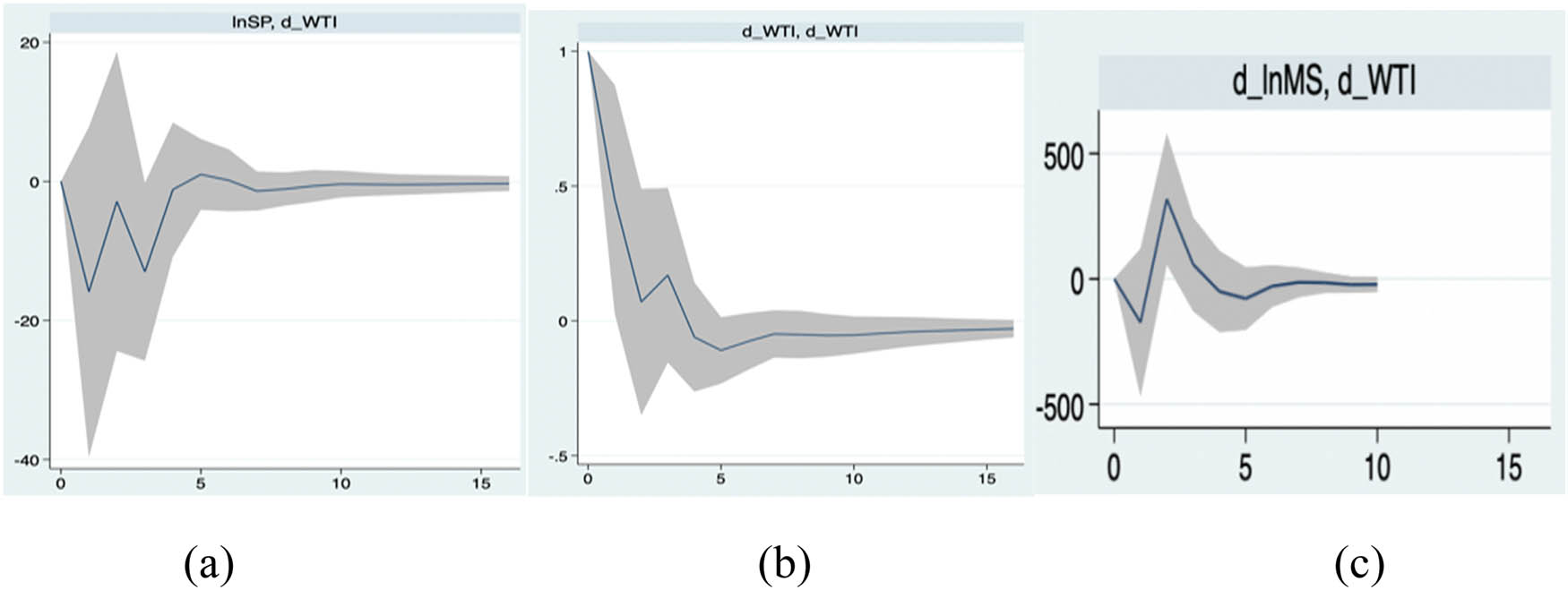
The graphs show the impact on oil price caused, by oil price (a), stock performance (b), and money supply (c). The shaded region represents 95% confidence interval.
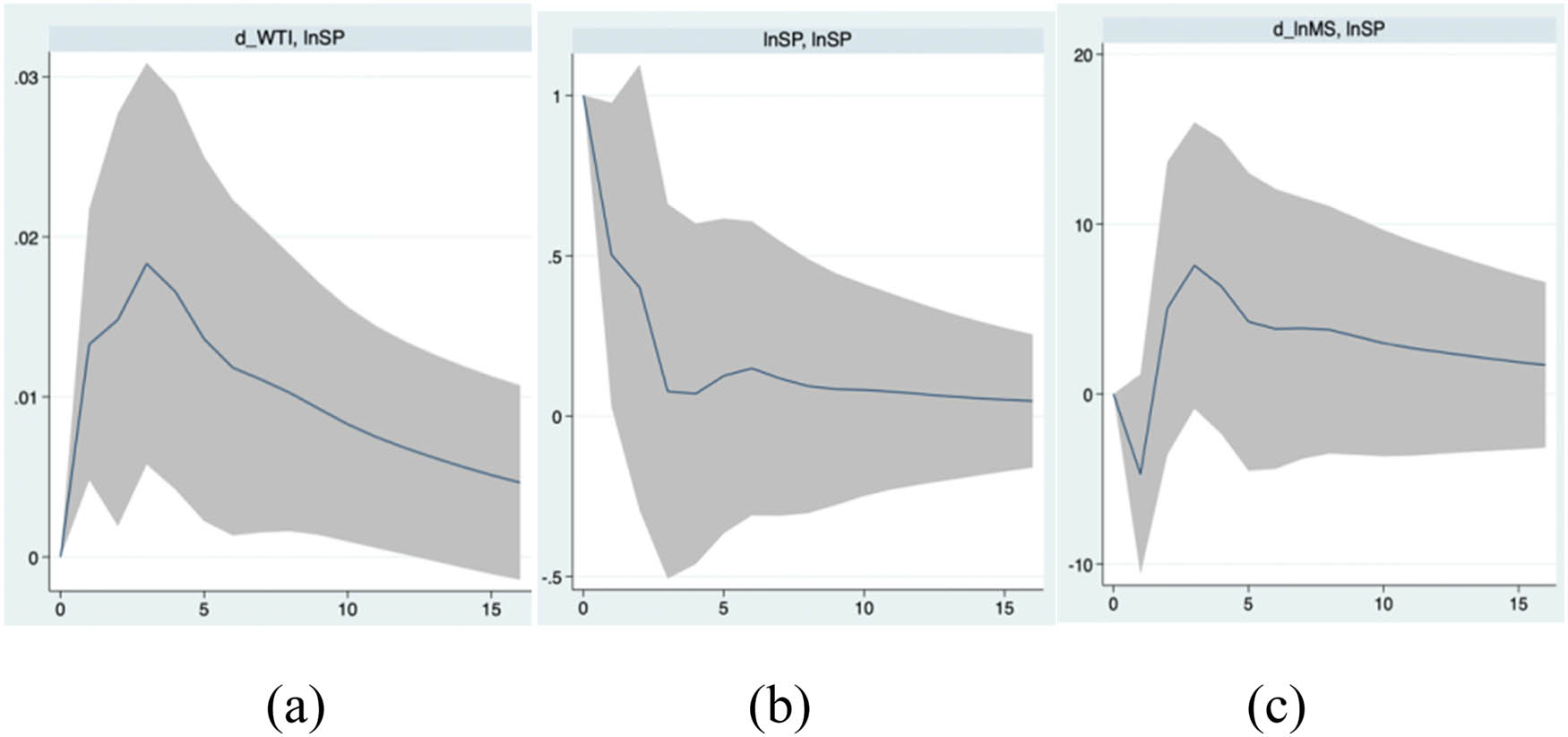
The graphs show the impact on stock performance caused, by oil price (a), stock performance (b), and money supply (c). The shaded region represents 95% confidence interval.
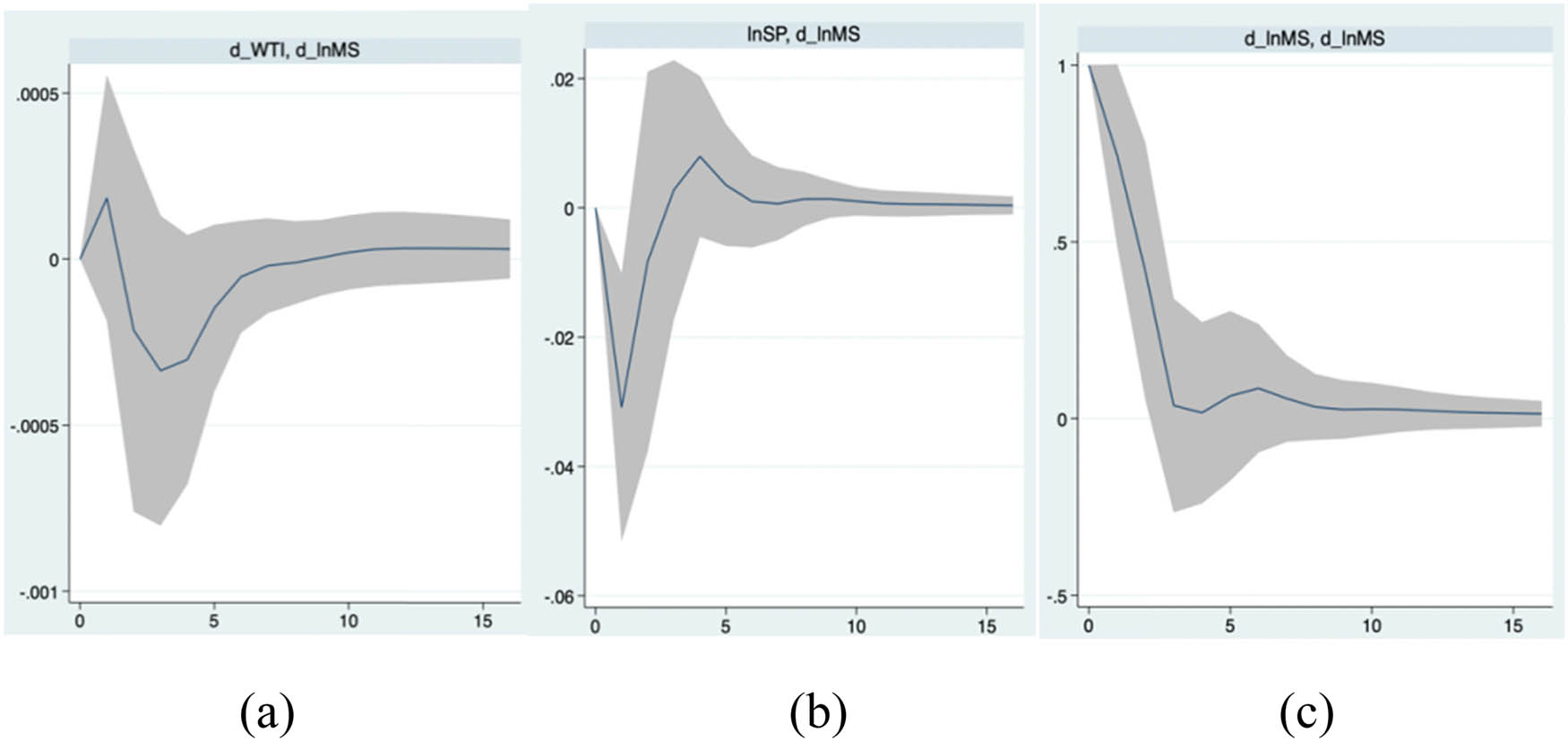
The graphs show the impact on money supply caused, by oil price (a), stock performance (b), and money supply (c). The shaded region represents 95% confidence interval.
The results of IRF analysis shed light on the interaction between the variables. The analysis shows that oil price responds to both stock performance and money supply. In the first five steps of IRF, the oil price would respond to a positive signal caused by stock performance, and the effect of the impulse gradually dampens after step 7. The fluctuation in oil price responding to stock price fluctuation shows that speculations play a role in the determination of future oil prices, which is supported by the work of Fawley et al. (2021). Although Granger causality test fails to identify stock performance as an explanatory factor of oil price, this does not interfere with the results yielded from IRF analysis due to the presence of inherent shortcomings of the test (Maziarz, 2015). Similarly, oil price responds strongly to an impulse of money supply. In the first five steps, oil price rises sharply to a positive impulse of money supply before dampening after step 7. This shows how oil price responds to expansionary monetary policy. Since expansionary monetary policies can cause economic boom and increase demand for oil, oil investors would invest more in oil future and cause oil price to rise, resulting in the IRF shown in Figure 1(c).
The IRF of stock performance shows the factors that affect the variable. In the first five steps, a positive impulse of oil price would cause a minor increase in stock performance before its effects dampen after step 5. This is somewhat different from the results from Granger causality test because the effects of oil price fluctuation on stock performance are not reflected by IRF analysis. However, money supply does have significant impact: In the first five steps, a positive impulse of money supply would result in an increase in stock performance. Since expansionary monetary policy would often result in economic recovery and expansion, the stock market would naturally react positively to the change.
Finally, the results of money supply to impulses show that money supply is overall independent from oil price fluctuation and is slightly influenced by stock market performance. As shown in Figure 3(a), a positive impulse in oil price fails to result in a significant change in the money supply. However, a positive impulse in stock performance does cause money supply to drop slightly in the first three steps. Money supply drops because of contractionary monetary policies, which are usually used by the central bank to slow down the overheating economy that can be signaled by rising stock prices. Overall, results from IRF analysis on money supply match those yielded by Granger causality test.
4.6 Variance Decomposition Analysis
The variance decomposition analysis of VAR model can reveal important information regarding the relative importance of random information. The key process is to decompose the variance of endogenous variables in the model into components that can be explained by other variables in the model and therefore substantiate the extent of impact on endogenous variables caused by other variables in the model (Omisakin, 2008). This research utilizes STATA to complete the variance decomposition analysis for oil price, stock performance, and money supply with a total of five steps.
As shown in Tables 8–10, the variance decomposition analysis provides new insights into factors that can explain the variance of the variables in the VAR model and is overall consistent with results yielded from previous analysis.
Results of variance decomposition of oil price with a step of 5
| Step | Oil price | Stock performance | Money supply |
|---|---|---|---|
| 1 | 1 | 0 | 0 |
| 2 | 0.983 | 0.005 | 0.012 |
| 3 | 0.910 | 0.041 | 0.049 |
| 4 | 0.887 | 0.064 | 0.048 |
| 5 | 0.887 | 0.064 | 0.049 |
Results of the variance decomposition of stock performance with a step of 5
| Step | Oil price | Stock performance | Money supply |
|---|---|---|---|
| 1 | 0.719 | 0.281 | 0 |
| 2 | 0.814 | 0.177 | 0.010 |
| 3 | 0.862 | 0.124 | 0.014 |
| 4 | 0.870 | 0.105 | 0.025 |
| 5 | 0.877 | 0.093 | 0.029 |
Results of variance decomposition of money supply with a step of 5
| Step | Oil price | Stock performance | Money supply |
|---|---|---|---|
| 1 | 0.048 | 0.395 | 0.557 |
| 2 | 0.152 | 0.476 | 0.373 |
| 3 | 0.214 | 0.442 | 0.344 |
| 4 | 0.245 | 0.424 | 0.330 |
| 5 | 0.254 | 0.420 | 0.325 |
First, the results of variance decomposition of oil price show that in the first five steps, the majority of the variance in oil price can be accounted for by oil price itself, but the other two variables still account for almost 10% of the variance of oil price, substantiating their impact on oil prices. This is consistent with the results from Granger causality test and IRF analysis that stock price and money supply have noticeable influence on oil price, although the intensity and duration of such impact are not persistent. Combined, the results indicate that oil price is influenced not only by its own supply–demand interaction but also by macroeconomic changes indicated by other economic variables.
Second, the variance decomposition of stock performance indicates the role played by oil price in inducing variance in stock prices. In the first five steps, oil price accounts for more than 80% of the variance in stock performance, while money supply plays a relatively minor role. This is different from outcomes in IRF, where money supply is identified as a greater impacting factor on stock performance. Still, both tests show that stock prices are somewhat correlated and influenced by oil price and money supply changes. An increase in the money supply will affect stock prices through a series of economic variables. Initially, it caused a temporary negative impact on the stock price, causing the stock price to decline, and then a strong positive impact, driving the stock price to rise. Subsequently, the impact decreased, or even decreased to a negative value, indicating that the stock market would fluctuate under the impact of the money supply. An increase in the price level will also cause the stock price to rise first and then fall. Theoretically, rising price levels, i.e., increasing inflation, will lead to the devaluation of the currency held by residents. The awareness of maintaining value will encourage people to spend more money to purchase financial assets and real estate, thereby driving up stock prices. However, as inflation continues to increase, the currency continues to depreciate, resulting in a large amount of currency issuance, leading to excess liquidity. At this time, inflation has a greater inhibitory effect on stock prices than a stimulating effect, leading to a decline in stock prices. An increase in interest rates will have a negative impact on stock prices, which will briefly raise stock prices, followed by a negative impact on stock prices. This is basically consistent with the trend of increasing the money supply’s impact on stock prices and is inconsistent with practical experience. The main reason for this phenomenon is that in the past interest rate, marketization was low. Only when economic development deviated from the normal track, the central bank would adjust and control the economy by changing interest rates, and there was a significant time lag in this regulation.
Lastly, the variance decomposition of money supply confirmed the impact of stock performance variation on money supply. In the first five lags, the percentage of variance of money supply that can be accounted for stock performance first increases from 0.395 to 0.476 before gradually decreasing. This corresponds to the results of both Granger causality test and IRF analysis, which both indicate stock performance as a factor that has a significant impact on money supply. The major difference between variance decomposition and IRF on money supply is the role played by oil price. While the IRF function suggests that oil price has a weak impact on money supply, variance decomposition suggests that the influence of oil price on money supply was significant, although not as substantial as stock performance and money supply itself. Such difference stems from the fact that the fundamental mechanisms of the models are different, which naturally lead to some discrepancies in the results generated. This would invite a combined analysis of results yielded from Granger causality test, IRF, and variance decomposition analysis, which should be presented in the conclusion.
5 Conclusion
To conclude, this research has established a VAR model to analyze the interactive relationship between oil price, stock performance, and money supply. Granger causality test, IRF analysis, and variance decomposition have been applied to the model to understand the specific interactive relationships between the variables. The main finding of the research is that oil price responds to changes in stock performance and money supply, stock performance is affected by both oil price and money supply, and money supply is influenced by stock performance. These relationships can help facilitate transactions in e-commerce, which happens at a faster pace and relies on more accurate prediction results.
First, the results of the model and analysis suggest that oil price responds to changes in stock performance (lnSP) and money supply (d_lnMS). Granger causality test identifies money supply as an explanatory factor of oil price; IRF analysis indicates that oil price would respond to impulses of both stock performance and money supply; variance decomposition analysis substantiates that a relatively small yet significant proportion of variance in oil price can be attributed to stock performance and money supply changes. Therefore, it can be reasonably concluded that oil price responds to changes in stock performance and money supply. Results from the analysis emphasize the effect of speculation in the determination of oil prices. Rather than solely determined by the supply and demand of oil, oil prices can be influenced by the speculation of traders who invest in oil futures and contracts. As the IRF analysis indicates, oil price would respond to changes in stock price and rise when the money supply increases. Increased money supply usually means expansionary monetary policy and a better economic outlook, creating the speculation that oil demand would increase as more economic transactions happen. This would cause oil price to rise and match outcomes yielded from empirical analysis. Based on the results of the tests, traders of oil futures in e-commerce should pay attention to fluctuations in stock performance and money supply, given the interactive relationship between the variables.
Second, the impact of oil price and money price on stock performance, as indicated by S&P 500 index, has been proven. Granger causality test indicates that both oil price and money supply are explanatory factors of stock market performance; IRF shows that positive impulse in oil price and money supply can result in an increase in stock performance; variance decomposition credits majority of variance in stock performance to oil price fluctuations. While the analysis together indicates that oil price and money supply can both influence stock price, they suggest different degrees of influence: IRF suggests a minor influence of oil price and a significant influence of money supply, while variance decomposition attributes majority of the variance in stock performance to oil price changes. Regardless, it can be concluded that both oil price and money supply can influence stock performance, which has been demonstrated by many previous studies summarized in the literature review. The conclusion is consistent with economic theory: As oil price rises, the stock value of oil companies would rise, driven stock prices up in the first few time periods. As the IRF analysis reveals, the rise in stock performance caused by a rise in oil price would diminish after a few time periods because companies that manufacture products that use oil as a raw material are harmed by higher production costs resulting from oil price hike. The positive relationship between stock performance and money supply is more obvious because the increase in money supply signals expansionary monetary policy that can boost business confidence and stock performance. For this reason, traders of stocks in e-commerce should keep in mind fluctuations in oil price and money supply to prevent losses.
Finally, the VAR model and resulting analysis proved the connection between stock market performance and money supply. Granger causality test shows that stock market performance (lnSP) is an explanatory factor of money supply; IRF demonstrates that money supply would decrease to a positive impulse of lnSP; variance decomposition shows that a significant portion of the variance of money supply can be explained by stock performance. The results show that money supply, although it should be independent from government and public opinion, does respond to changes in stock market performance. A positive change in stock market performance would often signal economic expansion, so contractionary monetary policies that are carried out by decreasing money supply are used to prevent the economy from overheating. This explains the negative relationship between stock market performance and money supply indicated by the analysis.
In addition to the variables featured in the research, there are many factors that affect the interaction between oil price, stock performance, and money supply. For instance, policy and psychology can play a role in such interaction. Due to limited time and energy, the author does not consider the impact of these factors one by one but only considers the interactions between oil price, stock performance, and money supply. Considering the impact of macroeconomy and other factors on these three variables from a comprehensive and multi-angle perspective, as well as establishing economic models, is a long and arduous process, and it is also an urgent issue to be resolved in future research work. Moreover, the research could benefit from using other empirical analyses to examine the effectiveness and validity of the VAR model.
-
Funding information: The author(s) received no financial support for the research, authorship, and/or publication of this article.
-
Conflict of interest: The authors have no relevant financial or nonfinancial interests to disclose.
-
Article note: As part of the open assessment, reviews and the original submission are available as supplementary files on our website.
-
Data availability statement: The datasets generated and/or analyzed during the current study are available from the corresponding author on reasonable request.
References
Akaike, H. (1998). Information theory and an extension of the maximum likelihood principle. In Selected papers of Hirotugu Akaike (pp. 199–213). New York, NY: Springer New York.10.1007/978-1-4612-1694-0_15Search in Google Scholar
Board of Governors of the Federal Reserve System. (2023a, October 24). M2. FRED. https://fred.stlouisfed.org/series/M2SL.Search in Google Scholar
Bollerslev, T. (1986). Generalized autoregressive conditional heteroskedasticity. Journal of Econometrics, 31(3), 307–327.10.1016/0304-4076(86)90063-1Search in Google Scholar
Box, G. E., Jenkins, G. M., Reinsel, G. C., & Ljung, G. M. (2015). Time series analysis: forecasting and control. John Wiley & Sons.Search in Google Scholar
Cologni, A., & Manera, M. (2008). Oil prices, inflation and interest rates in a structural cointegrated VAR model for the G-7 countries. Energy Economics, 30(3), 856–888.10.1016/j.eneco.2006.11.001Search in Google Scholar
Cong, R. G., Wei, Y. M., Jiao, J. L., & Fan, Y. (2008). Relationships between oil price shocks and stock market: An empirical analysis from China. Energy Policy, 36(9), 3544–3553.10.1016/j.enpol.2008.06.006Search in Google Scholar
Degiannakis, S., Filis, G., & Panagiotakopoulou, S. (2018). Oil price shocks and uncertainty: How stable is their relationship over time?. Economic Modelling, 72, 42–53.10.1016/j.econmod.2018.01.004Search in Google Scholar
Delgado, N. A. B., Delgado, E. B., & Saucedo, E. (2018). The relationship between oil prices, the stock market and the exchange rate: Evidence from Mexico. The North American Journal of Economics and Finance, 45, 266–275.10.1016/j.najef.2018.03.006Search in Google Scholar
Diks, C., & Panchenko, V. (2006). A new statistic and practical guidelines for nonparametric Granger causality testing. Journal of Economic Dynamics and Control, 30(9–10), 1647–1669.10.1016/j.jedc.2005.08.008Search in Google Scholar
de Castro Sobrosa Neto, R., de Lima, C. R. M., Bazil, D. G., & de Andrade Guerra, J. B. S. O. (2020). Sustainable development and corporate financial performance: A study based on the Brazilian Corporate Sustainability Index (ISE). Sustainable Development, 28(4), 960–977.10.1002/sd.2049Search in Google Scholar
Du, L., Yanan, H., & Wei, C. (2010). The relationship between oil price shocks and China’s macro-economy: An empirical analysis. Energy Policy, 38(8), 4142–4151.10.1016/j.enpol.2010.03.042Search in Google Scholar
Eltony, M. N., & Al‐Awadi, M. (2001). Oil price fluctuations and their impact on the macroeconomic variables of Kuwait: A case study using a VAR model. International Journal of Energy Research, 25(11), 939–959.10.1002/er.731Search in Google Scholar
Faisal, S. M. (2021). Overview of the ARIMA model average crude oil price forecast and its implications on the Indian economy post-liberalization. International Journal of Multidisciplinary: Applied Business and Education Research, 2(2), 118–127.10.11594/ijmaber.02.02.06Search in Google Scholar
Fan, Y., Zhang, Y. J., Tsai, H. T., & Wei, Y. M. (2008). Estimating ‘Value at Risk’ of crude oil price and its spillover effect using the GED-GARCH approach. Energy Economics, 30(6), 3156–3171.10.1016/j.eneco.2008.04.002Search in Google Scholar
Farjamnia, I., Naseri, M., & Ahmadi, S. M. M. (2007). Oil price forecasting; A comparison between ARIMA and ANN models. Iranian Journal of Economic Research, 9(32), 161–183.Search in Google Scholar
Fawley, B. W., Juvenal, L., & Petrella, I. (2021, December 9). When oil prices jump, is speculation to blame?: St. Louis Fed. Saint Louis Fed Eagle. http://www.stlouisfed.org/publications/regional-economist/april-2012/when-oil-prices-jump-is-speculation-to-blame.Search in Google Scholar
Galindo-Martín, M. Á., Castaño-Martínez, M. S., & Méndez-Picazo, M. T. (2021). Effects of the pandemic crisis on entrepreneurship and sustainable development. Journal of Business Research, 137, 345–353.10.1016/j.jbusres.2021.08.053Search in Google Scholar
Giot, P., & Laurent, S. (2003). Market risk in commodity markets: A VaR approach. Energy Economics, 25(5), 435–457.10.1016/S0140-9883(03)00052-5Search in Google Scholar
Granger, C. W. (1969). Investigating causal relations by econometric models and cross-spectral methods. Econometrica: Journal of the Econometric Society, 3, 424–438.10.2307/1912791Search in Google Scholar
Hammoudeh, S., & Aleisa, E. (2004). Dynamic relationships among GCC stock markets and NYMEX oil futures. Contemporary Economic Policy, 22(2), 250–269.10.1093/cep/byh018Search in Google Scholar
Hou, A., & Suardi, S. (2012). A nonparametric GARCH model of crude oil price return volatility. Energy Economics, 34(2), 618–626.10.1016/j.eneco.2011.08.004Search in Google Scholar
S&P 500 historical rates (SPX). Investing.com. (2022). http://www.investing.com/indices/us-spx-500-historical-data.Search in Google Scholar
Jebabli, I., Arouri, M., & Teulon, F. (2014). On the effects of world stock market and oil price shocks on food prices: An empirical investigation based on TVP-VAR models with stochastic volatility. Energy Economics, 45, 66–98.10.1016/j.eneco.2014.06.008Search in Google Scholar
Kilishi, A. A. (2010). Oil price shocks and the Nigeria economy: A variance autoregressive (VAR) model. International Journal of Business and management, 5(8), 39.10.5539/ijbm.v5n8p39Search in Google Scholar
Klein, T., & Walther, T. (2016). Oil price volatility forecast with mixture memory GARCH. Energy Economics, 58, 46–58.10.1016/j.eneco.2016.06.004Search in Google Scholar
Korosteleva, J. (2022). The implications of Russia’s invasion of Ukraine for the EU energy market and businesses. British Journal of Management, 33(4), 1678–1682.10.1111/1467-8551.12654Search in Google Scholar
Leneenadogo, W., & Lebari, T. (2019). Modelling the Nigeria crude oil prices using ARIMA, pre-intervention and post-intervention model. Asian Journal of Probability and Statistics, 3(1), 1–12.10.9734/ajpas/2019/v3i130083Search in Google Scholar
Mahmoudi, M., & Ghaneei, H. (2022). Detection of structural regimes and analyzing the impact of crude oil market on Canadian stock market: Markov regime-switching approach. Studies in Economics and Finance, 39(4), 722–734.10.1108/SEF-09-2021-0352Search in Google Scholar
Martishin, E. M., Gladkaya, S. V., Yeletsky, A. N., Zotova, T. A., & Yatsenko, A. B. (2022). Evolutionary management in managing economic growth and sustainable development. In Innovative trends in international business and sustainable management (pp. 363–371). Singapore: Springer Nature Singapore.10.1007/978-981-19-4005-7_40Search in Google Scholar
Maziarz, M. (2015). A review of the Granger-causality fallacy. The Journal of Philosophical Economics: Reflections on Economic and Social Issues, 8(2), 86–105.10.46298/jpe.10676Search in Google Scholar
Nademi, A., & Nademi, Y. (2018). Forecasting crude oil prices by a semiparametric Markov switching model: OPEC, WTI, and Brent cases. Energy Economics, 74, 757–766.10.1016/j.eneco.2018.06.020Search in Google Scholar
Nyangarika, A., Mikhaylov, A., & Henning Richter, U. (2019). Influence oil price towards macroeconomic indicators in Russia. International Journal of Energy Economics and Policy, 9(1), 123–129.Search in Google Scholar
Omisakin, D. O. A. (2008). Oil price shocks and the Nigerian economy: A forecast error variance decomposition analysis. Journal of Economic Theory, 2(4), 124–130.Search in Google Scholar
Ono, S. (2011). Oil price shocks and stock markets in BRICs. The European Journal of Comparative Economics, 8(1), 29–45.Search in Google Scholar
Pan, X. Z., Ma, X. R., Wang, L. N., Lu, Y. C., Dai, J. Q., & Li, X. (2022). Spillover of international crude oil prices on China’s refined oil wholesale prices and price forecasting: Daily-frequency data of private enterprises and local refineries. Petroleum Science, 19(3), 1433–1442.10.1016/j.petsci.2022.03.013Search in Google Scholar
Sadorsky, P. (1999). Oil price shocks and stock market activity. Energy Economics, 21(5), 449–469.10.1016/S0140-9883(99)00020-1Search in Google Scholar
Schwarz, G. (1978). Estimating the dimension of a model. The Annals of Statistics, 6, 461–464.10.1214/aos/1176344136Search in Google Scholar
Singhal, S., & Ghosh, S. (2016). Returns and volatility linkages between international crude oil price, metal and other stock indices in India: Evidence from VAR-DCC-GARCH models. Resources Policy, 50, 276–288.10.1016/j.resourpol.2016.10.001Search in Google Scholar
Sims, C. A. (1980). Macroeconomics and reality. Econometrica: Journal of the Econometric Society, 48, 1–48.10.2307/1912017Search in Google Scholar
U.S. Energy Information Administration: West Texas Intermediate (WTI) - cushing, Oklahoma. FRED. (2023, November 1). https://fred.stlouisfed.org/series/DCOILWTICO.Search in Google Scholar
Wang, Y., Wu, C., & Yang, L. (2013). Oil price shocks and stock market activities: Evidence from oil-importing and oil-exporting countries. Journal of Comparative Economics, 41(4), 1220–1239.10.1016/j.jce.2012.12.004Search in Google Scholar
Xiang, Y., & Zhuang, X. H. (2013). Application of ARIMA model in short-term prediction of international crude oil price. Advanced Materials Research, 798, 979–982.10.4028/www.scientific.net/AMR.798-799.979Search in Google Scholar
Yildirim, Z., & Arifli, A. (2021). Oil price shocks, exchange rate and macroeconomic fluctuations in a small oil-exporting economy. Energy, 219, 119527.10.1016/j.energy.2020.119527Search in Google Scholar
Yu, L., Wang, S., & Lai, K. K. (2005). A rough-set-refined text mining approach for crude oil market tendency forecasting. International Journal of Knowledge and Systems Sciences, 2(1), 33–46.Search in Google Scholar
© 2024 the author(s), published by De Gruyter
This work is licensed under the Creative Commons Attribution 4.0 International License.
Articles in the same Issue
- Regular Articles
- Political Turnover and Public Health Provision in Brazilian Municipalities
- Examining the Effects of Trade Liberalisation Using a Gravity Model Approach
- Operating Efficiency in the Capital-Intensive Semiconductor Industry: A Nonparametric Frontier Approach
- Does Health Insurance Boost Subjective Well-being? Examining the Link in China through a National Survey
- An Intelligent Approach for Predicting Stock Market Movements in Emerging Markets Using Optimized Technical Indicators and Neural Networks
- Analysis of the Effect of Digital Financial Inclusion in Promoting Inclusive Growth: Mechanism and Statistical Verification
- Effective Tax Rates and Firm Size under Turnover Tax: Evidence from a Natural Experiment on SMEs
- Re-investigating the Impact of Economic Growth, Energy Consumption, Financial Development, Institutional Quality, and Globalization on Environmental Degradation in OECD Countries
- A Compliance Return Method to Evaluate Different Approaches to Implementing Regulations: The Example of Food Hygiene Standards
- Panel Technical Efficiency of Korean Companies in the Energy Sector based on Digital Capabilities
- Time-varying Investment Dynamics in the USA
- Preferences, Institutions, and Policy Makers: The Case of the New Institutionalization of Science, Technology, and Innovation Governance in Colombia
- The Impact of Geographic Factors on Credit Risk: A Study of Chinese Commercial Banks
- The Heterogeneous Effect and Transmission Paths of Air Pollution on Housing Prices: Evidence from 30 Large- and Medium-Sized Cities in China
- Analysis of Demographic Variables Affecting Digital Citizenship in Turkey
- Green Finance, Environmental Regulations, and Green Technologies in China: Implications for Achieving Green Economic Recovery
- Coupled and Coordinated Development of Economic Growth and Green Sustainability in a Manufacturing Enterprise under the Context of Dual Carbon Goals: Carbon Peaking and Carbon Neutrality
- Revealing the New Nexus in Urban Unemployment Dynamics: The Relationship between Institutional Variables and Long-Term Unemployment in Colombia
- The Roles of the Terms of Trade and the Real Exchange Rate in the Current Account Balance
- Cleaner Production: Analysis of the Role and Path of Green Finance in Controlling Agricultural Nonpoint Source Pollution
- The Research on the Impact of Regional Trade Network Relationships on Value Chain Resilience in China’s Service Industry
- Social Support and Suicidal Ideation among Children of Cross-Border Married Couples
- Asymmetrical Monetary Relations and Involuntary Unemployment in a General Equilibrium Model
- Job Crafting among Airport Security: The Role of Organizational Support, Work Engagement and Social Courage
- Does the Adjustment of Industrial Structure Restrain the Income Gap between Urban and Rural Areas
- Optimizing Emergency Logistics Centre Locations: A Multi-Objective Robust Model
- Geopolitical Risks and Stock Market Volatility in the SAARC Region
- Trade Globalization, Overseas Investment, and Tax Revenue Growth in Sub-Saharan Africa
- Can Government Expenditure Improve the Efficiency of Institutional Elderly-Care Service? – Take Wuhan as an Example
- Media Tone and Earnings Management before the Earnings Announcement: Evidence from China
- Review Articles
- Economic Growth in the Age of Ubiquitous Threats: How Global Risks are Reshaping Growth Theory
- Efficiency Measurement in Healthcare: The Foundations, Variables, and Models – A Narrative Literature Review
- Rethinking the Theoretical Foundation of Economics I: The Multilevel Paradigm
- Financial Literacy as Part of Empowerment Education for Later Life: A Spectrum of Perspectives, Challenges and Implications for Individuals, Educators and Policymakers in the Modern Digital Economy
- Special Issue: Economic Implications of Management and Entrepreneurship - Part II
- Ethnic Entrepreneurship: A Qualitative Study on Entrepreneurial Tendency of Meskhetian Turks Living in the USA in the Context of the Interactive Model
- Bridging Brand Parity with Insights Regarding Consumer Behavior
- The Effect of Green Human Resources Management Practices on Corporate Sustainability from the Perspective of Employees
- Special Issue: Shapes of Performance Evaluation in Economics and Management Decision - Part II
- High-Quality Development of Sports Competition Performance Industry in Chengdu-Chongqing Region Based on Performance Evaluation Theory
- Analysis of Multi-Factor Dynamic Coupling and Government Intervention Level for Urbanization in China: Evidence from the Yangtze River Economic Belt
- The Impact of Environmental Regulation on Technological Innovation of Enterprises: Based on Empirical Evidences of the Implementation of Pollution Charges in China
- Environmental Social Responsibility, Local Environmental Protection Strategy, and Corporate Financial Performance – Empirical Evidence from Heavy Pollution Industry
- The Relationship Between Stock Performance and Money Supply Based on VAR Model in the Context of E-commerce
- A Novel Approach for the Assessment of Logistics Performance Index of EU Countries
- The Decision Behaviour Evaluation of Interrelationships among Personality, Transformational Leadership, Leadership Self-Efficacy, and Commitment for E-Commerce Administrative Managers
- Role of Cultural Factors on Entrepreneurship Across the Diverse Economic Stages: Insights from GEM and GLOBE Data
- Performance Evaluation of Economic Relocation Effect for Environmental Non-Governmental Organizations: Evidence from China
- Functional Analysis of English Carriers and Related Resources of Cultural Communication in Internet Media
- The Influences of Multi-Level Environmental Regulations on Firm Performance in China
- Exploring the Ethnic Cultural Integration Path of Immigrant Communities Based on Ethnic Inter-Embedding
- Analysis of a New Model of Economic Growth in Renewable Energy for Green Computing
- An Empirical Examination of Aging’s Ramifications on Large-scale Agriculture: China’s Perspective
- The Impact of Firm Digital Transformation on Environmental, Social, and Governance Performance: Evidence from China
- Accounting Comparability and Labor Productivity: Evidence from China’s A-Share Listed Firms
- An Empirical Study on the Impact of Tariff Reduction on China’s Textile Industry under the Background of RCEP
- Top Executives’ Overseas Background on Corporate Green Innovation Output: The Mediating Role of Risk Preference
- Neutrosophic Inventory Management: A Cost-Effective Approach
- Mechanism Analysis and Response of Digital Financial Inclusion to Labor Economy based on ANN and Contribution Analysis
- Asset Pricing and Portfolio Investment Management Using Machine Learning: Research Trend Analysis Using Scientometrics
- User-centric Smart City Services for People with Disabilities and the Elderly: A UN SDG Framework Approach
- Research on the Problems and Institutional Optimization Strategies of Rural Collective Economic Organization Governance
- The Impact of the Global Minimum Tax Reform on China and Its Countermeasures
- Sustainable Development of Low-Carbon Supply Chain Economy based on the Internet of Things and Environmental Responsibility
- Measurement of Higher Education Competitiveness Level and Regional Disparities in China from the Perspective of Sustainable Development
- Payment Clearing and Regional Economy Development Based on Panel Data of Sichuan Province
- Coordinated Regional Economic Development: A Study of the Relationship Between Regional Policies and Business Performance
- A Novel Perspective on Prioritizing Investment Projects under Future Uncertainty: Integrating Robustness Analysis with the Net Present Value Model
- Research on Measurement of Manufacturing Industry Chain Resilience Based on Index Contribution Model Driven by Digital Economy
- Special Issue: AEEFI 2023
- Portfolio Allocation, Risk Aversion, and Digital Literacy Among the European Elderly
- Exploring the Heterogeneous Impact of Trade Agreements on Trade: Depth Matters
- Import, Productivity, and Export Performances
- Government Expenditure, Education, and Productivity in the European Union: Effects on Economic Growth
- Replication Study
- Carbon Taxes and CO2 Emissions: A Replication of Andersson (American Economic Journal: Economic Policy, 2019)