A Proof of Proposition 1

For pa>ϕ , an a student’s expected productivity is positive for ga=1 . Conversely, a d student’s expected productivity is w0 for gd=pdμ−w01−pd1+w0 . Given the number of job positions J, each firm compares the expected profit obtained by high-grade students with different social background: this is EPagau=1>EPdgdu=pdμ−w01−pd1+w0=w0 . Hence, all the a students are preferred in the labour market (za=1 ), while the d students are hired for the remainder of job positions available. Therefore, disadvantaged high grade students are hired with probability zd that solves

This is non-negative by Assumption 1.1., while

for

We exclude the case where J≥Ju by Assumption 1.3.

For pa<ϕ , an i student’s expected productivity is non-negative for gi=piμ−w01−pi1+w0 . Comparing the expected profit obtained by A students with different social background yields EPagau=paμ−w01−pa1+w0=EPdgdu=pdμ−w01−pd1+w0=w0 . As a consequence, firms hire a and d students in the same proportion, i. e. za=zd=z , and

This is non-negative, and it is smaller than 1 for

Again, we exclude the case where J≥J2u by Assumption 1.3.

B A model with exogenous grading

In this section, we show that the results of the baseline model are consistent with a setting where the interaction between statistical discrimination among social groups and differences in grading is exogenous, and the school does not have a specific objective function. Suppose that the school assigns a grade based on a student’s performance at the exam, but the exam performance is not a perfect signal of academic achievement. A proportion of ka,kd∈0,1 advantaged and disadvantaged low-achievers score A at the final exam. Moreover, students of privileged backgrounds perform better relative to true achievement, so that ka>kd , due to their greater access to opportunities to prepare the exam well. According to Bayes rule, students’ expected productivities are:

When piμ−w01−pi1+w0>1⟺pi>ϕ , then EPi>w0 for every ki∈0,1 . Remember though that pd<ϕ by Assumption 1.2. Thus for pa>ϕ , the firms’ strategy is za=1 , while EPd≥w0 as long as kd≤pdμ−w01−pd1+w0 . Hence disadvantaged high grade students are hired with probability zd that solves

Hiring strategy eq. (6) of course decreases with kd until, at the limit, kd=pdμ−w01−pd1+w0 and the hiring decisions mirror those of the baseline model. The same applies when pa<ϕ .

C Specific objectives

In this section, we consider a government interested in fostering specific aspects of the economy, namely, the job opportunities of a specific social group, the economic efficiency, expressed by productivity, and wage equality. As in the main text, we compare the different policies, together with the unregulated equilibrium, to evaluate which intervention is most useful for each point. Notice that, if the introduction of a policy does not change the outcome of the unregulated case, we assume that the social planner refrains from intervening. This is because any policy entails some administrative and organisational costs, which are not modelled here for simplicity.

D Job opportunities by social group

Here we assume that the government aims at evaluating policies based on their effects on the number of job offers to a specific social group, oi . A couple of preliminary caveats must be considered. First, it is not enough to observe only the hiring strategy to infer the number of jobs offered, as this is based on the number of students who scored A, whose number changes according to the grading strategy.

Second, the interaction between school and firms ensures that all job positions J are filled in the range of interest in each equilibrium configuration. This is because the school objective function is to increase the job opportunities. By considering however an exogenous grading model (see the previous section), which has the advantage of not requiring any school objective, the results are qualitatively similar for job opportunities among social groups. For convenience, define:

Figure 3:

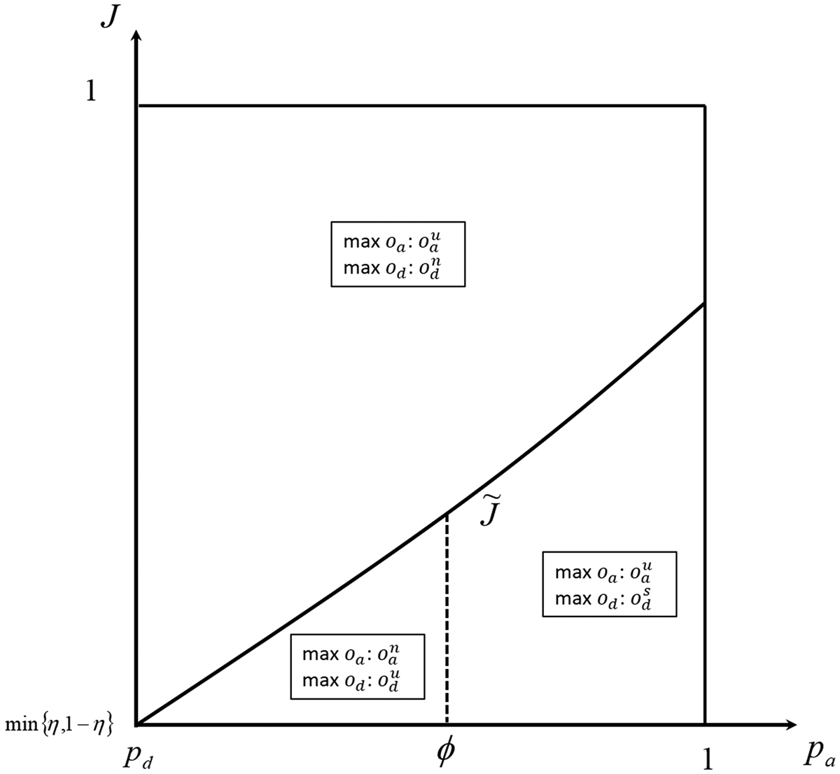
Job opportunities

Figure 3 illustrates which policy favours the job opportunities of a or d students, again in the space pa,J , in the relevant range. Each caption indicates which configuration ensures the maximum number of job offers for students coming from social group i. Proposition 6 shows that, when the social planner is concerned with the job opportunities of a specific social group, his best policy choice depends on the quality of human capital in the populations, i. e. the proportion of high achievers, together with the number of jobs available. Interestingly, with few job positions and a high number of high-achievers among the advantaged group, introducing an anti-grade salary policy favours advantaged students. Proposition 4 may help explaining this result. When there is a large proportion of high achievers among privileged students (pa>ϕ ) and the number of jobs is scarce (J<J˜ ), an anti-grade discrimination policy increases the expected productivity of a students compared to d students. In turn their appeal as labour market candidates increases. In this case, for instance, a social planner aiming at promoting the job opportunities of disadvantaged students should avoid any intervention.

E Salaries

In this section, we assume that the government is interested to compare policies according to their effects on salaries. As stressed above, the equilibrium salary corresponds to a student’s expected productivity, wi=EPigi for every i∈a,d . Therefore, unlike the analysis of job opportunities, here the hiring strategy does not play any role in determining the salary level. Moreover, since affirmative action does not affect the grading strategies, salaries do not change with the introduction of this policy compared to the unregulated equilibrium. Table 2 summarises equilibrium salaries:

To interpret the equilibrium salaries, note that the salary level is negatively related to grade inflation, as it lowers the expected productivity. This is consistent with the existing literature on grade inflation: as in Chan, Hao, and Suen (2007) and Schwager (2012), the presence of grade inflation hinders high-achievers in terms of salary. A quick check shows that pa1+μ−1>w0 for pa>ϕ . In addition,

for pa>ϕ , while

for pa<ϕ . We are now able to compare the different configurations.

The salaries of advantaged students are favoured by the adoption of an anti-grade discrimination policy, as this forces their grade inflation down. The effect is an increase in the expected productivity of advantaged students, who thus receive a better salary offer than in any other context. This result is consistent with the welfare analysis, according to which an anti-grade discrimination policy maximises welfare by raising the wages of advantaged students.

As for disadvantaged students, the introduction of an anti-wage discrimination policy is useful only when the difference in the distribution of achievement among advantaged and disadvantaged students is high, i.e. pa>ϕ . Otherwise, the presence of targeted grading is sufficient, without any policy intervention, to equate the salaries of students coming from different social groups.

F Inequality

We finally assume that the government aims at reducing inequality among social groups. The exercise here consists in comparing salaries of advantaged and disadvantaged students, wa−wd . Table 3 summarises the results.

By definition, the anti-wage discrimination policy prevents inequality on salaries, and thus it is the best choice for this goal. Notice also that, since affirmative action does not affect salaries, the adoption of this policy exhibits the same inequality level as the unregulated case. For pa>ϕ , comparing the level of inequalities with unregulated and anti-grade discrimination policy, we get

For pa<ϕ , the only policy that brings about inequalities is the anti-grade discrimination policy. The above discussion can be summarised as follows.

Proposition 8 shows that banning targeted grading spurs inequality in salaries, even if the introduction of this policy is welfare maximising. For pa<ϕ , no regulating intervention is necessary to contrast inequality. Indeed, targeted grading goes against the difference in the distribution of achievement among social groups, by raising the expected achievement of disadvantaged students at equilibrium and in turn their salaries.

G Proof of Lemma 1

Suppose otherwise. Then school maximisation implies a grading strategy that yields higher expected productivity of one group of students. Thus, a firm would strictly prefer to hire a student from this group. By Assumption 1.1., there are more jobs than such students. Hence competition among firms ensures that the wage is set to their expected productivity. As a consequence, the equilibrium wage will be higher than the expected productivity of the second group of students, who would not receive any job offer. This grading strategy would not maximise the number of employed students, by contradicting the initial hypothesis.

H Proof of Proposition 2

The condition to obtain same salaries at equilibrium is EPa=EPd . When pa>ϕ , the school may keep gas=1 as in the targeted case, and lower the level of gds until productivities are the same:

This strategy ensures the maximum level of hiring under the required constraint. Given the same productivity, firms hire a and d students in the same proportion, i. e. za=zd=z , and

This is non-negative, and it is smaller than 1 for

which holds by Assumption 1.3.

I Proof of Lemma 2

Suppose otherwise, then there are two cases. In the first case, firms may design a hiring policy, constrained by za=zd=zaf , according to the distribution of achievement of the privileged social group. Given pa>ϕ , the expected productivity of a students is higher than w0 for any level of ga . Therefore the school chooses ga=1 , as it increases the number of employed students, while firms choose zaf=1 , as in Proposition 1. However, since the hiring strategy will be the same also for underprivileged students, the school has an incentive in raising the level of grade inflation for d students to gd=1 , thus driving the expected productivity of d students to be lower than the reservation utility and equal to

It follows that all students from the disadvantaged population would refuse the job offer. Hence, in this case, zaf=za=1 , but zd=0 , which contradicts the initial assumption.

In the second case, firms may set zaf lower than one but higher than zdu . Yet, the school still has an incentive to inflate grades more than gdu=pdμ−w01−pd1+w0 , yielding again, at equilibrium, a salary offer to d students lower than their reservation utility, with zaf≠zd=0 , again a contradiction. This continuation equilibrium would drive firms to hire students coming from the two social groups according to the distribution of achievement of disadvantaged students.

J Proof of Proposition 3

The affirmative action policy requires that hiring must be the same across social groups, za=zd=z . By Lemma 2, the hiring policy must be based on the distribution of achievement of underprivileged students. Also, since the affirmative action does not put any restrictions on students’ expected productivity, then the school will keep the same grading strategy as in the unregulated case. For pa>ϕ and ga=1, gd=pdμ−w01−pd1+w0 , high grade students are hired with probability z that solves

Finally, zaf<1 for J<J1u , which holds by Assumption 1 .3.

K Proof of Lemma 3

Suppose otherwise. Then, the school will maximise the number of job offers subject to ga=gd according to the expected productivity of advantaged students. For pa>ϕ , this implies gin=1 by Proposition 1, while firms choose zan=1 . However, this level of grade inflation will drive the expected productivity of underprivileged students below their reservation utility, since EPdgd=1=pdμ−1−pd<w0 . In turn, all students from the disadvantaged population would refuse the job offer, so that zdn=0 . Hence this grading strategy does not maximise the number of employed students, by contradicting the initial hypothesis.

For pa<ϕ , a grading policy based on the expected productivity of advantaged students is

by Proposition 1.In this case, the expected productivities are

where

Following the previous reasoning, the optimal recruiting strategy is again zan=1,zdn=0 .

L Proof of Proposition 4

Here we assume that grading cannot be targeted across social groups, ga=gd=g . By Lemma 3, the best grading strategy is determined according to the distribution of achievement of disadvantaged students, irrespective of the value of pa . A d student’s expected productivity is non-negative for gn=pdμ−w01−pd1+w0 . Any grading policy g′>gn implies that none of the d students receives any job offer, as their expected productivity would be negative.

The grading policy gn=pdμ−w01−pd1+w0 entails EPagn=pdμ−w01−pd1+w0>EPdgn=pdμ−w01−pd1+w0 for every pd . Thus, all the privileged high grade students receive a job offer (zan=1 ), while disadvantaged high grade students are hired for the remainder of job positions: they are hired with probability zdn that solves

Finally, notice that zdn<1 for

As usual, point 3 of Assumption 1 ensures that this holds.

M Proof of Proposition 6

The results at equilibrium can be used to determine the job opportunities for each social group i∈a,d , i.e.:

For each range of pa , we begin by listing the job opportunities in each possible equilibrium configuration. We will then compare the four cases: unregulated equilibrium, anti-wage discrimination policy, affirmative action policy and anti-wage discrimination policy. It is useful to remember that Assumption 1.3. implies J<minJ1u,Js,Jaf,Jn .

Case pa>ϕ

Consider first the unregulated equilibrium where the school is free to target grades and there are no restrictions on salaries. This is oau=η and odu=J−η . When an anti-wage discrimination policy is implemented, the job opportunities are oas=η and ods=pd1−ηJηpa+1−ηpd . When an affirmative action policy is implemented, the job opportunities are,

Finally, consider the case where an anti-grade discrimination policy is implemented:

We are now in a position to examine the different job opportunities. Comparing the different configurations, we get, for advantaged students:

while

For disadvantaged students,

and

Finally, odn>ods for J>J˜ , where

Case pa<ϕ

The job opportunities with unregulated equilibrium are

The job opportunities do not change compared the unregulated equilibrium when introducing either an anti-wage discrimination or an affirmative action policy, oiu=ois=oiaf . As for the anti-grade discrimination policy, the job opportunities are the same as in eqs. (8) and (9).

Comparing the unregulated equilibrium with the anti-grade discrimination policy for advantaged students, we get

for J>J˜ . For disadvantaged students,

for J>J˜ .

References

Allahar, A., and J. Côté. 2007. The Ivory Tower Blues, 195–98. Toronto: University of Toronto.Suche in Google Scholar
Arrow, K. J. 1973. “The Theory of Statistical Discrimination.” In Discrimination in Labor Markets, edited by Ashenfelter and Rees. Princeton, NJ: Princeton University Press.Suche in Google Scholar
Bar, T., V. Kadiyali, and A. Zussman. 2012. “Put Grades in Context.” Journal of Labor Economics 30 (2): 445–78.10.1086/663591Suche in Google Scholar
Burgess, S., and E. Greaves. 2013. “Test Scores, Subjective Assessment and Stereotyping of Ethnic Minorities.” Journal of Labor Economics 31: 535–76.10.1086/669340Suche in Google Scholar
Carneiro, P., and J. J. Heckman. 2003. “Human Capital Policy”. In Inequality in America: What Role for Human Capital Policies?, edited by J. J. Heckman, and A. B. Krueger. The MIT Press.10.2139/ssrn.434544Suche in Google Scholar
Chan, W., L. Hao, and W. Suen. 2007. “A Signalling Theory of Grade Inflation.” International Economic Review 48: 1065–90.10.1111/j.1468-2354.2007.00454.xSuche in Google Scholar
Coate, S., and G. C. Loury. 1993. “Will Affirmative-Action Policies Eliminate Negative Stereotypes?” American Economic Review 83: 1220–40.Suche in Google Scholar
Cunha, F., J. J. Heckman, L. Lochner, and D. V. Masterov. 2006. “Interpreting the Evidence on Life Cycle Skill Formation.” Handbook of the Economics of Education 1, chapter 12: 697–812.10.3386/w11331Suche in Google Scholar
Dee, T. S., W. Dobbie, B. A. Jacob, and J. Rockoff. 2016. “The Causes and Consequences of Test Score Manipulation: Evidence from the New York Regents Examinations.” NBER Working Paper 22165.10.3386/w22165Suche in Google Scholar
Ehlers, T., and R. Schwager. 2016. “Honest Grading, Grade Inflation and Reputation.” CESifo Economic Studies 62: 506–21.10.1093/cesifo/ifv022Suche in Google Scholar
Figlio, D., and M. Lucas. 2004. “Do High Grading Standards Affect Student Performance?” Journal of Public Economics 88: 1815–34.10.3386/w7985Suche in Google Scholar
Hanna, R. N., and L. L. Linden. 2012. “Discrimination in Grading.” American Economic Journal: Economic Policy 4: 146–68.10.1257/pol.4.4.146Suche in Google Scholar
Higher Education Statistic Agency. Graduate Info in year 1996/97 and 2008/09.Suche in Google Scholar
Himmler, O., and R. Schwager. 2013. “Double Standards in Educational Standards: Are Disadvantaged Students Being Graded More Leniently?” German Economic Review 14: 166–89.10.2139/ssrn.975022Suche in Google Scholar
Hodgen, J., D. Kuchemann, M. Brown, and R. Coe. 2009. “Children’s Understandings of Algebra 30 Years on.” Research in Mathematics Education 11: 193–94.10.1080/14794800903063653Suche in Google Scholar
Singer. 2015. Welcome to the 2015 Recruiter Nation, Formerly Known as the Social Recruiting Survey. https://www.jobvite.com/jobvite-news-and-reports/welcome-to-the-2015-recruiter-nation-formerly-known-as-the-social-recruiting-survey/.Suche in Google Scholar
Johnson, V. E. 2003. Grade Inflation: A Crisis in College Education. New York: Springer-Verlag.Suche in Google Scholar
Joshi, H. E., and A. McCulloch. 2001. “Neighbourhood and Family Influences on the Cognitive Ability of Children in the British National Child Development Study.” Social Science and Medicine 53: 579–91.10.1016/S0277-9536(00)00362-2Suche in Google Scholar
Kiss, D. 2010. “Are Immigrants Graded Worse in Primary and Secondary Education? Evidence for German Schools.” Ruhr Economic Paper 223, RWI - Leibniz-Institut für Wirtschaftsforschung, Ruhr-University Bochum, TU Dortmund University, University of Duisburg-Essen.10.2139/ssrn.1711873Suche in Google Scholar
Lavy, V., and R. Megalokonomou. 2017. “Persistency in Teachers’ Grading Biases and Effect on Longer Term Outcomes: University Admission Exams and Choice of Field of Study.” Unpublished Manuscript.Suche in Google Scholar
Lavy, V., and E. Sand. 2015. “On the Origins of Gender Human Capital Gaps: Short and Long Term Consequences of Teachers’ Stereotypical Biases.” NBER Working Paper 20909.10.3386/w20909Suche in Google Scholar
Lüdemann, E., and G. Schwerdt. 2010. “Migration Background and Educational Tracking: Is There a Double Disadvantage for Second-Generation Immigrants?” Journal of Population Economics 26: 455–81.10.1007/s00148-012-0414-zSuche in Google Scholar
MacLeod, B. W., and M. Urquiola. 2015. “Reputation and School Competition.” American Economic Review 105: 3471–88.10.1257/aer.20130332Suche in Google Scholar
Modica, S. 2008. “I voti di laurea non sono normali.” La Voce. http://www.lavoce.info/articoli/pagina1000421-351.html.Suche in Google Scholar
Moro, A., and P. Norman. 2003. “Affirmative Action in a Competitive Economy.” Journal of Public Economics 87: 567–94.10.1016/S0047-2727(01)00121-9Suche in Google Scholar
Moro, A., and P. Norman. 2004. “A General Equilibrium Model of Statistical Discrimination.” Journal of Economic Theory 114: 1–30.10.1016/S0022-0531(03)00165-0Suche in Google Scholar
Norman, P. 2003. “Statistical Discrimination and Efficiency.” Review of Economic Studies 70: 615–27.10.1111/1467-937X.00258Suche in Google Scholar
Popov, S. V., and D. Bernhardt. 2013. “University Competition and Grading Standards.” Economic Inquiry 51: 1764–78.10.1111/j.1465-7295.2012.00491.xSuche in Google Scholar
Prenzel, M., J. Baumert, W. Blum, R. Lehmann, D. Leutner, M. Neubrand, Reinhard Pekrun, Jurgen Rost, and Ulrich Schiefele. 2003 PISA 2003 Ergebnisse des zweiten internationalen Vergleichs – Zusammenfassung, IPN - Leibniz-Institut für die Pädagogik der Naturwissenschaften an der Universität Kiel http://pisa.ipn.uni-kiel.de/Zusammenfassung\_2003.pdf.Suche in Google Scholar
Rojstaczer, S., and C. Healy. 2012. Teachers College Record 7. http://www.tcrecord.org.Suche in Google Scholar
Rosovsky, H., and M. Hartley. 2002. Evaluation and the Academy: Are We Doing the Right Thing? Cambridge, MA: American Academy of Arts and Sciences.Suche in Google Scholar
Schwager. 2012. “Grade Inflation, Social Background and Labour Market Matching.” Journal of Economic Behavior and Organization 82: 56–66.10.1016/j.jebo.2011.12.012Suche in Google Scholar
U.K. Parlament. Equal Pay Act 1970.Suche in Google Scholar
U.S. Equal Employment Opportunity Commission.Equal Pay Act of 1963.Suche in Google Scholar
Yang, H., and C.S. Yip. 2003. “An Economic Theory of Grade Inflation.” Working paper, University of Pennsylvania.Suche in Google Scholar
Wikström, C., and M. Wikström. 2005. “Grade Inflation and School Competition: An Empirical Analysis based on the Swedish upper Secondary Schools.” Economic of Education Review 24: 309–22.10.1016/j.econedurev.2004.04.010Suche in Google Scholar
© 2019 Walter de Gruyter GmbH, Berlin/Boston
Artikel in diesem Heft
- Research Articles
- Optimal Forestry Contract with Interdependent Costs
- Bi and Branching Strict Nash Networks in Two-way Flow Models: A Generalized Sufficient Condition
- Pay-What-You-Want in Competition
- Two Rationales for Insufficient Entry
- Students’ Social Origins and Targeted Grading
- Pricing, Signalling, and Sorting with Frictions
- On the Economic Value of Signals
- The Core in Bertrand Oligopoly TU-Games with Transferable Technologies
- Reasoning About ‘When’ Instead of ‘What’: Collusive Equilibria with Stochastic Timing in Repeated Oligopoly
- Timing Games with Irrational Types: Leverage-Driven Bubbles and Crash-Contingent Claims
- Costly Rewards and Punishments
- Blocking Coalitions and Fairness in Asset Markets and Asymmetric Information Economies
- Strategic Activism in an Uncertain World
- On Equilibrium Existence in a Finite-Agent, Multi-Asset Noisy Rational Expectations Economy
- Optimal Incentives Under Gift Exchange
- Public Good Indices for Games with Several Levels of Approval
- Vagueness of Language: Indeterminacy under Two-Dimensional State-Uncertainty
- Winners and Losers of Universal Health Insurance: A Macroeconomic Analysis
- Behavioral Theory of Repeated Prisoner’s Dilemma: Generous Tit-For-Tat Strategy
- Flourishing as Productive Tension: Theory and Model
- Notes
- A Note on Reference-Dependent Choice with Threshold Representation
- Regular Equilibria and Negative Welfare Implications in Delegation Games
- Unbundling Production with Decreasing Average Costs
- A Simple and Procedurally Fair Game Form for Nash Implementation of the No-Envy Solution
- Decision Making and Games with Vector Outcomes
- Capital Concentration and Wage Inequality
- Annuity Markets and Capital Accumulation