Generalized quasi-linear fractional Wentzell problems
-
Efren Mesino-Espinosa


Abstract
Given a bounded
where
1 Introduction
Let
We now introduce the boundary value problem under consideration in this work. Consider the following quasi-linear Wentzell-type problem, explicitly given by
where
The existence and uniqueness of a weak solution to problem (
The global boundedness of weak solutions of problem (
A
A weak comparison principle for solution to the boundary value problem (
A nonlinear Fredholm alternative associated with the equation (
In view of the above formulations, we address several important main observations concerning our equation of interest. First, we observe that problem (
for
For the classical local problem involving the
Fractional Wentzell-type boundary value problems are barely known. For the linear case (
Fractional Laplacian-type operators are very important in probability, as they are generators of
The study is organized as follows. Section 2 reviews the fundamental concepts, definitions, and known results, which will be applied in the subsequent sections. Some particular examples of non-smooth domains having the structure suitable for the study are also given in this section. In Section 3, we first state the main assumptions that will be carried out throughout the study, and then we proceed to stablish the unique solvability of problem (
2 Preliminaries
We state fundamental concepts, notations, and important tools for the development of the work in this study. We introduce some function spaces along with their essential properties. We also define fractional Sobolev spaces and Besov spaces and provide some embedding theorems. Furthermore, we introduce the regional fractional
2.1
(
ε
,
δ
)
-domains and
d
-sets
Here we will introduce two key concepts about sets that will be considered in the development of this research. For a deeper exploration of these concepts, readers are encouraged to refer [23,24].
Definition 1
[23] Let
We say that
Definition 2
[24] A closed non-empty set
The measure
Examples of sets fulfilling both of the above definitions include many non-smooth and non-Lipschitz domains, as shown here.
2.2 Fractional Sobolev spaces, Besov spaces, and other function spaces
In this section, we will introduce the concepts of fractional Sobolev spaces and Besov spaces. Additionally, we will discuss some important properties of these spaces that are essential for the development of this work. For more information, please refer [8,10,15,24,25,28,38].
First, given
Definition 3
[28,38] Let
endowed with the norm
Theorem 4
[28] The fractional Sobolev space
Definition 5
[8,9] Let
endowed with the norm
Theorem 6
[24] The Besov space
For the domains under consideration in this study, a characterization of the trace space of
Theorem 7
[8,24] Let
there exists a continuous linear operator Ext from
Definition 8
[28] Let
It is known that if
Theorem 9
[8, Theorem 1.6] Let
In some instances, for
endowed with the norm
and, if
2.3 Embedding theorems
The following embedding results are important and will be highly applied throughout the rest of the study. We will present results regarding fractional Sobolev spaces and Besov spaces.
First, we set
We first state the interior embedding result.
Theorem 10
[10, Theorem 6.7] Let
that is, the space
For the next result, we use the first part of [9, Theorem 11.1] together with the extension property and the fact that
Theorem 11
[9] Let
Remark 12
Let
From [33], one can clearly deduce that
Since the maps
(2.5)and
(2.6)for each
If
2.4 Regional fractional
p
-Laplacian
In this section, we focus on the regional fractional
Definition 13
[38] Let
Definition 14
[38] Let
provided that the limit exists. Where the positive normalized constant
and
Now, we introduce the notion of
Theorem 15
(Fractional Green formula; [8, Theorem 2.2]) Let
and its boundary
where
Remark 16
Note that if
2.5 Examples of domains
We now collect some examples of non-smooth regions exhibiting the required conditions for the validity of Theorem 15.
Example 17
We present three concrete examples of non-Lipschitz domains fulfilling all the conditions mentioned in Theorem 15.
The most known example of a locally uniform domain with fractal boundary (and thus failing to be a Lipschitz domain) is the classical Koch snowflake domain in
We consider ramified domains over
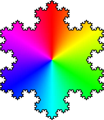
The two-dimensional Koch snowflake domain.
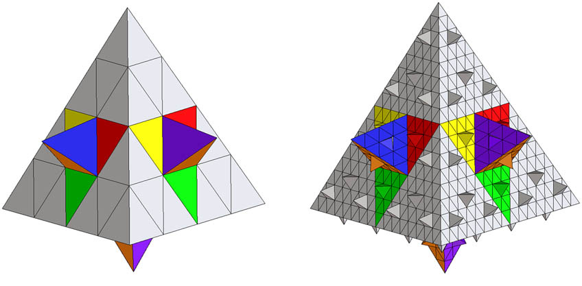
Koch 4-crystal
![Figure 3
A T-shaped domain (refer [1]) on the left-hand side and a domain with ramified fractal boundary in the critical case
a
=
a
∗
≃
0.593465
a={a}^{\ast }\simeq 0.593465
(refer [2]) on the right-hand side.](/document/doi/10.1515/anona-2025-0110/asset/graphic/j_anona-2025-0110_fig_003.jpg)
2.6 Some analytical tools
We close this section by presenting some analytical results, which will be very helpful in the subsequent sections of this study.
Lemma 18
[11] Let
for
where
Proposition 19
[5] Let
If in addition
and also, in this case, there is a constant
For
Finally, if
and
Proposition 20
[5] Let
3 Solvability
The aim of this section is to establish existence and uniqueness for weak solutions of the boundary value problem (
- (3.1)
The boundary
Next define the following nonlinear forms:
and
Then, we have the following result for the above form.
Lemma 21
The (nonlinear) form given by (3.2) satisfies
Proof
Fix
In the same way, we deduce that
For the local terms, first we apply Theorem 10 to infer that
for some constant
for some
for all
which shows that
Proving that
where
Taking
We then distinguish two cases:
Combining the above inequality with (3.9), it follows that
and thus from the above inequality with (3.9), it follows that
Therefore,
From (3.7) and (3.12), we deduce that
Since
proving that
Now, we will prove the existence and uniqueness of weak solutions to problem (
Theorem 22
Let
where
Proof
The conclusions of Lemma 21 imply particularly that for every
where
Because
A straightforward application of Hölder’s inequality together with Theorems 10 and 11 shows that
for some constant
4 A priori estimates
In this section, we are fully devoted in establishing
To begin, given
Since it is well known that the spaces
For a set
Clearly
Lemma 23
Let
If
If
Now, we are ready to give the main result of this section.
Theorem 24
Let
and
If
If
where
for
Proof
We will only prove part (b) (since part (a) follows in an easier manner). Let
where
We will assume that
Then, we define the following sets:
Then, we clearly see that
Apply Proposition 19 and Lemma 23 when necessary, for
By rearranging the above calculations, we obtain that
and by virtue of (4.6), equation (4.7) becomes
Applying Proposition 20 for
it follows that
Combining (4.9) with Lemma 23, we obtain that
Taking
Also, note that from Theorems 10,11, and the definition of the space
for
for all
and selecting
Then, substituting the previous expression in equation (4.10) results in
Letting
for
Now, by (3.7) and (4.15), we have that
Since
where
Now, on the right side of inequality (4.18), we must deal with the expression
Recalling our assumption
Substituting (4.20) in (4.18), and applying Young’s inequality, we deduce that
where
It follows that
Note that
so rewriting (4.21) and substituting (4.22), we obtain that
Applying Theorems 10 and 11 on the left-hand side of (4.23), we have that
where
Next given
Thus, combining (4.25) and (4.24), we deduce that
Setting
from (4.26), it follows that
Since
and henceforth, it follows from (4.28) that
Clearly
Applying Lemma 18 to the function
we obtain that
for some constant
and thus,
From here, combining (4.30) and (4.31), we have that
where
for some constant
Finally, combining all possibilities in this case, we can conclude that there exists a constant
such that
establishing our desired result for the case
Proceeding as before, we calculate and arrive at
As
where
for any
Selecting
Taking
Recalling the definition of
Since
it follows (similarly as in the previous case) that there exists a constant
Applying Lemma 18 to the function
we obtain that
for some constant
where
and
where
where
and consequently,
and
Substituting (4.45) and (4.46) in (4.44) gives that
where
Now, proceeding similarly as to the previous cases, if we take
Using again the function
As
we obtain that
for some constant
gives that
for some constant
where
Equation (4.52) establishes the desired result for the case
and
where
Therefore, by combining these four cases, we have proven the desired result.□
5 Maximum principle
In this section, we explore inverse positivity and a weak comparison principle for solutions of the boundary value problem (
To begin, consider the differential inequality, formally given by
where
Definition 25
A function
where
and the nonlinear form
Our first result shows that weak solutions to differential inequality (5.1) are globally nonnegative. We recall that for a measurable function
Theorem 26
Let
Proof
Let
Then, testing (5.2) with the function
Since
and thus,
Furthermore, by (3.7), there exists a constant
Combining (5.3) and (5.4), we deduce that
Taking into account the previous result, we can easily derive the following result on inverse positivity.
Corollary 27
Let
To conclude this section, we introduce a fundamental tool for analyzing the behavior of weak solutions to problem (
Theorem 28
Given
Proof
Given
and thus,
On the other hand, clearly
In particular, choosing
it follows that
Next in either
Taking into account this latest calculation, the definitions of
we obtain that
Consequently,
and similarly,
Now, for
Clearly
and similarly,
From (5.5), together with (5.7), (5.8), (5.9), and (5.10), we conclude that
Since each term in (5.11) has the same sign, this implies that
and
In the last two integrals, each term within them has a defined sign, so this implies that
6 Nonlinear Fredholm alternative
In this section, we establish a sort of “nonlinear Fredholm alternative” for our problem, assuming the conditions and structures given in (A). To begin, we define the sets
It follows that
The following simple result shows that the fractional and Besov semi-norms become norms when restricted to the spaces
Proposition 29
The norms
define equivalent norms for the spaces
Proof
If
where
We now define the Banach space
endowed with the norm
defines an equivalent norm for the space
Next we define the functional
with effective domain
Proposition 30
Let
Remark 31
Observe that the variational formulation of equation (6.4) is given by
for all
In the next two results, we establish a relation between the null space of the operator
Lemma 32
Let
that is,
Proof
By Lemma 30, we have that
First, assume that
The above equality implies that
Lemma 33
The range of the operator
Proof
Let
In particular, by setting
from which it follows that
Conversely, let
endowed with the norm
where
By Hölder’s inequality and the norm equivalence given in (6.2), it follows that
and the above inequality implies that
This result implies that
where
From this, we deduce that
which shows that the functional
Hence,
Applying the Lebesgue Dominated Convergence Theorem, we obtain
Changing
Now, let
for all
We are now ready to state and prove the main result of this section.
Theorem 34
The operator
Acknowledgments
We would like to thank Dr. Yves Achdou and Dr. Nicoletta Tchou for their help in providing us with suitable images of ramified domains.
-
Funding information: The second author (the corresponding author) was supported by The Puerto Rico Science, Technology and Research Trust, under agreement number 2022-00014, and by University of Puerto Rico - R\'io Piedras FIPI grant 2024-2026, award number 20FIP1570025.
-
Author contributions: All authors have accepted responsibility for the entire content of this manuscript and consented to its submission to the journal, reviewed all the results, and approved the final version of the manuscript. Alejandro Vélez-Santiago (corresponding author) was the author of the idea of the project, which was given to Efren Mesino-Espinosa (first author) as a topic for his Master’s thesis. Therefore, the first author worked out most of the calculations and derivations of the manuscript under continuous guidance of the corresponding author. All the statements and calculations were refined further by the corresponding author, who also built the introduction section. Combining these procedures, we were able to complete the current manuscript.
-
Conflict of interest: The authors state no conflict of interest.
-
Disclaimer: This content is only the responsibility of the authors and does not necessarily represent the official views of The Puerto Rico Science, Technology and Research Trust.
References
[1] Y. Achdou, C. Sabot, and N. Tchou, A multiscale numerical method for Poisson problems in some ramified domains with a fractal boundary, Multiscale Model. Simul. 5 (2006), 828–860, https://doi.org/10.1137/05064583X. Suche in Google Scholar
[2] Y. Achdou and N. Tchou, Trace results on domains with self-similar fractal boundaries, J. Math. Pures Appl. 89 (2008), 596–623, https://doi.org/10.1016/j.matpur.2008.02.008. Suche in Google Scholar
[3] D. Applebaum, Lévy Processes and Stochastic Calculus, Cambridge University Press, Cambridge, 2011, https://doi.org/10.1017/CBO9780511809781. Suche in Google Scholar
[4] H. Attouch, G. Buttazzo, and G. Michaille, Variational analysis in Sobolev and BV spaces: applications to PDEs and optimization, MOS-SIAM Series on Optimization, Society for Industrial and Applied Mathematics, 2014, https://doi.org/10.1137/1.9781611973488. Suche in Google Scholar
[5] M. Biegert, A priori estimates for the difference of solutions to quasi-linear elliptic equations, Manuscripta Math. 133 (2010), 273–306, https://doi.org/10.1007/s00229-010-0367-z. Suche in Google Scholar
[6] C. Carvajal-Ariza, J. Henríquez-Amador, and A. Vélez-Santiago, The generalized anisotropic dynamical Wentzell heat equation with nonstandard growth conditions, J. Anal. Math. 154 (2024), 615–668, https://doi.org/10.1007/s11854-023-0306-z. Suche in Google Scholar
[7] Z. -Q. Chen and T. Kumagai, Heat kernels estimates for stable-like processes on d-sets, Stochastic Process. Appl. 108 (2003), 27–62, https://doi.org/10.1016/S0304-4149(03)00105-4. Suche in Google Scholar
[8] S. Creo and M. R. Lancia, Fractional (s,p)-Robin-Venttsel’ problems on extension domains, NoDEA Nonlinear Differential Equations Appl. 28 (2021), 31, https://doi.org/10.1007/s00030-021-00692-w. Suche in Google Scholar
[9] D. Danielli, N. Garofalo, and D. M. Nhieu, Non-doubling Ahlfors measures, perimeter measures, and the characterization of the trace spaces of Sobolev functions in Carnot-Carathéodory spaces, vol. 182, Memoirs of the American Mathematical Society, Providence, 2006, https://doi.org/10.1090/memo/0857. Suche in Google Scholar
[10] E. Di Nezza, G. Palatucci, and E. Valdinoci, Hitchhiker’s guide to the fractional Sobolev spaces, Bull. Sci. Math. 136 (2012), 521–573, https://doi.org/10.1016/j.bulsci.2011.12.004. Suche in Google Scholar
[11] V. Díaz-Martínez and A. Vélez-Santiago, Generalized anisotropic elliptic Wentzell problems with nonstandard growth conditions, Nonlinear Anal. Real World Appl. 68 (2022), 103689, https://doi.org/10.1016/j.nonrwa.2022.103689. Suche in Google Scholar
[12] P. Drábek and J. Milota, Methods of Nonlinear Analysis: Applications to Differential Equations, Birkhäuser, Basel, 2007. Suche in Google Scholar
[13] Q. Du, M. Gunzburger, and R. B. Lehoucq, A nonlocal vector calculus, nonlocal volume-constrained problems, and nonlocal balance laws, Math. Models Methods Appl. Sci. 23 (2013), 493–540, https://doi.org/10.1142/S0218202512500546. Suche in Google Scholar
[14] Q. Du, M. Gunzburger, and R. B. Lehoucq, Analysis and approximation of nonlocal diffusion problems with volume constraints, SIAM Rev. 54 (2012), 667–696, https://doi.org/10.1137/1108332. Suche in Google Scholar
[15] D. E. Edmunds and W. D. Evans, Fractional Sobolev Spaces and Inequalities, Cambridge University Press, Cambridge, 2022, https://doi.org/10.1017/9781009254625. Suche in Google Scholar
[16] G. Ferrer and A. Vélez-Santiago, 3D Koch-type crystals, J. Fractal Geom. 10 (2023), 109–149, 10.4171/JFG/130. Suche in Google Scholar
[17] C. G. Gal and M. Warma, Nonlinear elliptic boundary value problems at resonance with nonlinear Wentzell-Robin type boundary conditions, Adv. Math. Phys. 2017 (2017), 1–20, https://doi.org/10.1155/2017/5196513. Suche in Google Scholar
[18] C. G. Gal and M. Warma, Elliptic and parabolic equations with fractional diffusion and dynamic boundary conditions, Evol. Equ. Control Theory 5 (2016), 61–103, 10.3934/eect.2016.5.61. Suche in Google Scholar
[19] C. H. Gu and Y. B. Tang, Well-posedness of Cauchy problems of fractional drift diffusion system in non-critical spaces with power-law nonlinearity, Adv. Nonlinear. Anal. 13 (2024), 20240023, https://doi.org/10.1515/anona-2024-0023. Suche in Google Scholar
[20] Q. Y. Guan, Integration by parts formula for regional fractional Laplacian, Comm. Math. Phys. 266 (2006), 289–329, https://doi.org/10.1007/s00220-006-0054-9. Suche in Google Scholar
[21] M. Guerrero-Laos, E. Mesino-Espinosa, F. Seoanes, and A. Vélez-Santiago. Wentzell-type fractional heat equations: solvability and L∞-regularity, Preprint (2025). Suche in Google Scholar
[22] M. Gunzburger and R. B. Lehoucq, A nonlocal vector calculus with application to nonlocal boundary value problems, Multiscale Model. Simul. 8 (2010), 1581–1598, https://doi.org/10.1137/090766607. Suche in Google Scholar
[23] P. W. Jones, Quasiconformal mappings and extendability of functions in Sobolev spaces, Acta Math. 147 (1981), 71–88, 10.1007/BF02392869. Suche in Google Scholar
[24] A. Jonsson and H. Wallin, Function Spaces on Subsets of Rn, Part 1, Mathematics Reports, 2, Harwood Academic Publishers, London, 1984. Suche in Google Scholar
[25] A. Jonsson, Besov Spaces on Closed Subsets of Rn, Trans. Amer. Math. Soc. 341 (1994), 355–370, https://doi.org/10.2307/2154626. Suche in Google Scholar
[26] M. R. Lancia, A. Vélez-Santiago, and P. Vernole, A quasi-linear nonlocal Venttsel’ problem of Ambrosetti-Prodi type on fractal domains, Discrete Contin. Dyn. Syst. 39 (2019), 4487–4518, 10.3934/dcds.2019184. Suche in Google Scholar
[27] M. R. Lancia, A. Vélez-Santiago, and P. Vernole, Quasi-linear Venttsel’ problems with nonlocal boundary conditions on fractal domains, Nonlinear Anal. Real World Appl. 35 (2017), 265–291, https://doi.org/10.1016/j.nonrwa.2016.11.002. Suche in Google Scholar
[28] G. Leoni, A First Course in Fractional Sobolev Spaces, Graduate Studies in Mathematics, vol. 105, American Mathematical Society, Providence, 2009, 607 pp. 10.1090/gsm/105/10Suche in Google Scholar
[29] E. Mesino-Espinosa, Generalized Quasi-linear Fractional Venttsel’-type Problems Over Non-smooth Regions, Master’s Thesis, University of Puerto Rico - Mayagüez, 2024. Suche in Google Scholar
[30] R. Nittka, Elliptic and Parabolic Problems with Robin Boundary Conditions on Lipschitz Domains, Ph.D. Dissertation, Ulm, 2010. Suche in Google Scholar
[31] D. Schertzer, M. Larcheveque, J. Duan, V. V. Yanovsky, and S. Lovejoy, Fractional Fokker-Planck equation for nonlinear stochastic differential equations driven by non-Gaussian Lévy stable noises, J. Math. Phys. 42 (2001), 200–212, 10.1063/1.1318734. Suche in Google Scholar
[32] R. E. Showalter, Monotone Operators in Banach Space and Nonlinear Partial Differential Equations, American Mathematical Society, 2013. 10.1090/surv/049Suche in Google Scholar
[33] P. Shvartsman, On extensions of Sobolev functions defined on regular subsets of metric measure spaces, J. Approx. Theory 144 (2007), 139–161, https://doi.org/10.1016/j.jat.2006.05.005. Suche in Google Scholar
[34] K. Silva-Pérez and A. Vélez-Santiago, Diffusion over ramified domains: solvability and fine regularity, Calc. Var. Partial Differential Equations 64 (2025), 238, https://doi.org/10.1007/s00526-025-03103-5. Suche in Google Scholar
[35] A. Vélez-Santiago, Global regularity for a class of quasi-linear local and nonlocal elliptic equations on extension domains, J. Funct. Anal. 269 (2015), 1–46, https://doi.org/10.1016/j.jfa.2015.04.016. Suche in Google Scholar
[36] A. D. Venttsel, On boundary conditions for multidimensional diffusion processes, Theory Probab. Appl. 4 (1959), 164–177, 10.1137/1104014. Suche in Google Scholar
[37] H. Wallin, The trace to the boundary of Sobolev spaces on a snowflake, Manuscripta Math. 73 (1991), 117–125, https://doi.org/10.1007/BF02567633. Suche in Google Scholar
[38] M. Warma, The fractional Neumann and Robin type boundary conditions for the regional fractional p-Laplacian, NoDEA Nonlinear Differential Equations Appl. 23 (2016), 1–46, https://doi.org/10.1007/s00030-016-0354-5. Suche in Google Scholar
[39] M. Warma, The fractional relative capacity and the fractional Laplacian with Neumann and Robin boundary conditions on open sets, Potential Anal. 42 (2015), 499–547, https://doi.org/10.1007/s11118-014-9443-4. Suche in Google Scholar
© 2025 the author(s), published by De Gruyter
This work is licensed under the Creative Commons Attribution 4.0 International License.
Artikel in diesem Heft
- Research Articles
- Incompressible limit for the compressible viscoelastic fluids in critical space
- Concentrating solutions for double critical fractional Schrödinger-Poisson system with p-Laplacian in ℝ3
- Intervals of bifurcation points for semilinear elliptic problems
- On multiplicity of solutions to nonlinear Dirac equation with local super-quadratic growth
- Entire radial bounded solutions for Leray-Lions equations of (p, q)-type
- Combinatorial pth Calabi flows for total geodesic curvatures in spherical background geometry
- Sharp upper bounds for the capacity in the hyperbolic and Euclidean spaces
- Positive solutions for asymptotically linear Schrödinger equation on hyperbolic space
- Existence and non-degeneracy of the normalized spike solutions to the fractional Schrödinger equations
- Existence results for non-coercive problems
- Ground states for Schrödinger-Poisson system with zero mass and the Coulomb critical exponent
- Geometric characterization of generalized Hajłasz-Sobolev embedding domains
- Subharmonic solutions of first-order Hamiltonian systems
- Sharp asymptotic expansions of entire large solutions to a class of k-Hessian equations with weights
- Stability of pyramidal traveling fronts in time-periodic reaction–diffusion equations with degenerate monostable and ignition nonlinearities
- Ground-state solutions for fractional Kirchhoff-Choquard equations with critical growth
- Existence results of variable exponent double-phase multivalued elliptic inequalities with logarithmic perturbation and convections
- Homoclinic solutions in periodic partial difference equations
- Classical solution for compressible Navier-Stokes-Korteweg equations with zero sound speed
- Properties of minimizers for L2-subcritical Kirchhoff energy functionals
- Asymptotic behavior of global mild solutions to the Keller-Segel-Navier-Stokes system in Lorentz spaces
- Blow-up solutions to the Hartree-Fock type Schrödinger equation with the critical rotational speed
- Qualitative properties of solutions for dual fractional parabolic equations involving nonlocal Monge-Ampère operator
- Regularity for double-phase functionals with nearly linear growth and two modulating coefficients
- Uniform boundedness and compactness for the commutator of an extension of Riesz transform on stratified Lie groups
- Normalized solutions to nonlinear Schrödinger equations with mixed fractional Laplacians
- Existence of positive radial solutions of general quasilinear elliptic systems
- Low Mach number and non-resistive limit of magnetohydrodynamic equations with large temperature variations in general bounded domains
- Sharp viscous shock waves for relaxation model with degeneracy
- Bifurcation and multiplicity results for critical problems involving the p-Grushin operator
- Asymptotic behavior of solutions of a free boundary model with seasonal succession and impulsive harvesting
- Blowing-up solutions concentrated along minimal submanifolds for some supercritical Hamiltonian systems on Riemannian manifolds
- Stability of rarefaction wave for relaxed compressible Navier-Stokes equations with density-dependent viscosity
- Singularity for the macroscopic production model with Chaplygin gas
- Global strong solution of compressible flow with spherically symmetric data and density-dependent viscosities
- Global dynamics of population-toxicant models with nonlocal dispersals
- α-Mean curvature flow of non-compact complete convex hypersurfaces and the evolution of level sets
- High-energy solutions for coupled Schrödinger systems with critical growth and lack of compactness
- On the structure and lifespan of smooth solutions for the two-dimensional hyperbolic geometric flow equation
- Well-posedness for physical vacuum free boundary problem of compressible Euler equations with time-dependent damping
- On the existence of solutions of infinite systems of Volterra-Hammerstein-Stieltjes integral equations
- Remark on the analyticity of the fractional Fokker-Planck equation
- Continuous dependence on initial data for damped fourth-order wave equation with strain term
- Unilateral problems for quasilinear operators with fractional Riesz gradients
- Boundedness of solutions to quasilinear elliptic systems
- Existence of positive solutions for critical p-Laplacian equation with critical Neumann boundary condition
- Non-local diffusion and pulse intervention in a faecal-oral model with moving infected fronts
- Nonsmooth analysis of doubly nonlinear second-order evolution equations with nonconvex energy functionals
- Qualitative properties of solutions to the viscoelastic beam equation with damping and logarithmic nonlinear source terms
- Shape of extremal functions for weighted Sobolev-type inequalities
- One-dimensional boundary blow up problem with a nonlocal term
- Doubling measure and regularity to K-quasiminimizers of double-phase energy
- General solutions of weakly delayed discrete systems in 3D
- Global well-posedness of a nonlinear Boussinesq-fluid-structure interaction system with large initial data
- Optimal large time behavior of the 3D rate type viscoelastic fluids
- Local well-posedness for the two-component Benjamin-Ono equation
- Self-similar blow-up solutions of the four-dimensional Schrödinger-Wave system
- Existence and stability of traveling waves in a Keller-Segel system with nonlinear stimulation
- Existence and multiplicity of solutions for a class of superlinear p-Laplacian equations
- On the global large regular solutions of the 1D degenerate compressible Navier-Stokes equations
- Normal forms of piecewise-smooth monodromic systems
- Fractional Dirichlet problems with singular and non-locally convective reaction
- Sharp forced waves of degenerate diffusion equations in shifting environments
- Global boundedness and stability of a quasilinear two-species chemotaxis-competition model with nonlinear sensitivities
- Non-existence, radial symmetry, monotonicity, and Liouville theorem of master equations with fractional p-Laplacian
- Global existence, asymptotic behavior, and finite time blow up of solutions for a class of generalized thermoelastic system with p-Laplacian
- Formation of singularities for a linearly degenerate hyperbolic system arising in magnetohydrodynamics
- Linear stability and bifurcation analysis for a free boundary problem arising in a double-layered tumor model
- Hopf's lemma, asymptotic radial symmetry, and monotonicity of solutions to the logarithmic Laplacian parabolic system
- Generalized quasi-linear fractional Wentzell problems
- Existence, symmetry, and regularity of ground states of a nonlinear Choquard equation in the hyperbolic space
- Normalized solutions for NLS equations with general nonlinearity on compact metric graphs
- Boundedness and global stability in a predator-prey chemotaxis system with indirect pursuit-evasion interaction and nonlocal kinetics
- Review Article
- Existence and stability of contact discontinuities to piston problems