Compatibility of the method of brackets with classical integration rules
-
Zachary Bradshaw
 und
Christophe Vignat
und
Christophe Vignat

Abstract
The method of brackets is a symbolic approach to the computation of integrals over
1 Introduction
The problem of evaluating the definite integral
consists of expressing the value of
Example 1.1
For
is elementary. The only special function required is the primitive of
The aforementioned example is the most elementary case of the Fundamental theorem of Calculus.
Theorem 1.2
Assume g is a differentiable function on the interval
This result transforms the problem of evaluating the integral
Example 1.3
In order to evaluate the integral,
observe that
A simple generalization of this example shows that every polynomial
One of the main difficulties in the evaluation of definite integrals is the existence of elementary functions, such as those encountered in elementary courses, that do not have elementary primitives. In general, this is hard to establish. The notion of elementary function is left, for the purposes of this article, undefined. The reader will find in Ritt [1] more information about this topic.
Example 1.4
The symbolic language Mathematica gives the elementary evaluation
as well as the nonelementary one
where SinIntegral is the Mathematica notation for the sine integral function defined by:
Therefore, (1.7) simply comes from the introduction of a new function. The question of whether
2 The method of brackets
In the study of interaction of elementary particles, R. Feynman introduced his now famous diagrams, from which the physical properties of the reaction can be read. Some parametrizations of these diagrams led to families of quite complicated definite integrals.
A Feynman diagram is a graphical method of representing the interactions of elementary particles (see [2,3] for an introduction). For the present exposition, such a diagram is simply a graph
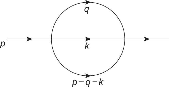
The massless sunset diagram.
Example
The massless sunset diagram is presented in Figure 1. The diagram is parametrized by the integral (in momentum space)
where
with
Several methods have been developed in order to deal with integrals of this form. The method of brackets used here is an effective variation of the method of negative dimension, one of the most used by the physics community, and consists of a small number of heuristic rules, some of which are in the process of being rigorously established. A complete description of the rules and a comparison with the current methods used to evaluate Feynman diagrams appear in [6].
This method of brackets computes the integral
from an expansion of the form
and introduces the bracket of
Formal replacement of series (2.4) in (2.3) expresses the integral as a bracket series:
In order to evaluate the integral, the method proposes a rule to assign a value to a bracket series.
Rule 1. For
A fundamental (open) question is to give a rigorous definition of this bracket, consistent with the operational rules in the following.
Rule 2. The expansion of an arbitrary function. The method of brackets requires the expansion of the integrand in the form:
where
For functions of several variables, say two, use the expansion
with the notation
Rule 3. Sum expansion. The expression
This has been established in [7], and it is a direct consequence of the multinomial theorem.
Up to now, the integral is converted into a bracket series. The evaluation of these series is described next.
Rule 4. Evaluation of bracket series. Let
where
Remark 2.1
Observe that this evaluation requires the evaluation of the coefficients
stated by S. Ramanujan’s in his Quarterly Reports [8, p. 298]. It was widely used by him as a tool in computing definite integrals and infinite series. In fact, as Hardy puts it in [9], he “was particularly fond of them, and used them as one of his commonest tools.”
Theorem 2.2
(Ramanujan’s Master Theorem). Let
An elementary argument adapts this statement to prove (2.11). See [10] for details.
Note
In the multidimensional evaluation of a bracket series, in the special case when the number of sums and brackets is the same, write
The multiple sum is declared to be
where
An inductive proof follows directly from the one-dimensional case.
3 Consistency with the fundamental theorem of calculus
This section shows that in the case, the integrand in (1.1) is a perfect derivative; then, the method of brackets is consistent with the fundamental theorem of calculus.
Theorem 3.1
The value of
Proof
Assume
and the last expression can be written as:
The change of variables
The system
coming from the vanishing of the brackets gives
Simplifying the previous summand gives
The proof is complete. The solutions corresponding to other combination of free variables yield the same result.□
4 The Laplace transform
A common variety of definite integrals appear as the Laplace transform of a function. This is defined by:
If the function
then
The next statement shows that (4.3) can be obtained directly by the method of brackets.
Theorem 4.1
The evaluation of the Laplace transform (4.1) by the method of brackets also produces (4.3).
Proof
The method of brackets gives
The vanishing of the bracket gives
confirming (4.3).□
5 Radially symmetric multidimensional integrals
This section confirms that an integral of the form
is evaluated correctly by the method of brackets.
The classical evaluation is performed using the
with
This gives
The last integral is
to produce
and using
The change of variables
The computation of
Then,
The associated linear system coming from the vanishing of the brackets is
The solution is
Using the method of brackets in the opposite order as usual yields
Then, (5.10) yields
as in (5.7).
6 Cauchy-Schlömilch transformation
In this section, we show that the method of brackets is consistent with the Cauchy-Schlömilch transformation.
Theorem 6.1
The method of brackets is consistent with the Cauchy-Schlömilch transformation. That is, using the method of brackets to evaluate the integrals, we have
Proof
Let
Similarly,
Thus, we have reduced (6.1) to the identity
Put another way, it suffices to consider even functions, for the odd part vanishes. Without loss of generality, let us assume that
and
Define
so that we have
Now applying the method of brackets, we find
The vanishing of the brackets produces three series, one for each choice of free index. These are
Since
Applying the method of brackets to this form of
The vanishing of the brackets produces three series, one for each choice of free index. These are
But these series exactly cancel the series arising from the first form of
Remark 6.2
An alternative form of the Schlömilch transformation on the half-line is usually written as:
Starting with the expansion
the usual procedure of the method of brackets evaluated the right-hand side as
and this is equivalent to
In order to evaluate the left-hand side of (6.23), start with
Rule 3 (sum expansion) of the method of brackets is now used to produce two expressions for the term
and
Replacing in (6.27) and using the standard rule for the method of brackets lead to three expressions for the integral
Index
This is discarded since every term vanishes.
Index
Index
The value of the desired integral is
7 Borwein integrals and an extension to Bessel functions
7.1 Borwein integrals
A Borwein integral is a definite integral of the form:
The integrals were introduced by David and Borwein in [12] and are somewhat famous for exhibiting consistency patterns that eventually break down. As an example, the following evaluations hold:
However, the pattern fails at the next step. Indeed, we have
The correct evaluation of the integral is off from
Now, applying the Legendre duplication formula, this becomes
Now, the vanishing of the bracket yields
where
Replacing in (7.13)
where
7.2 Extension to Bessel functions
The result on Borwein integrals can be extended to the integral of a product of Bessel functions. Indeed, recall the Bessel function of the first kind is given by:
Let us now compute
We have
Now, there are
where
Acknowledgements
Some of the results presented here are part of the doctoral dissertation of the first author. The last author wishes to thank the hospitality of the Mathematics Department of Tulane University while this work was being conducted.
-
Conflict of interest: The authors state no conflict of interest.
References
[1] J. F. Ritt, Integration in Finite Terms. Liouville’s Theory of Elementary Functions, Columbia University Press, New York, 1948. 10.7312/ritt91596Suche in Google Scholar
[2] M. Polyak, Feynman diagrams for pedestrians and mathematicians, In: M Lyubich, L. Takhtajan (Eds.), Graphs and Patterns in Mathematics and Theoretical Physics, Vol. 73, Proceedings of Symposia in Pure Mathematics, American Mathematical Society, USA, 2005. 10.1090/pspum/073/2131010Suche in Google Scholar
[3] M. Veltman, Diagrammatica. The Path to Feynman Diagrams, Vol. 4, Cambridge Lecture Notes in Physics, Cambridge University Press, Cambridge, 1994. 10.1017/CBO9780511564079Suche in Google Scholar
[4] M. E. Peskin and D. V. Schroder, An Introduction to Quantum Field Theory, CRC Press, Boca Raton, 2019. 10.1201/9780429503559Suche in Google Scholar
[5] L. A. Takhtadzhyan, Quantum Mechanics for Mathematicians, American Mathematical Society, Providence, 2008. Suche in Google Scholar
[6] K. VanDusen, A Comparison of Negative-Dimensional Integration Techniques, PhD thesis, Tulane University, Louisiana, 2021. Suche in Google Scholar
[7] I. Gonzalez and V. H. Moll, Definite integrals by the method of brackets. Part 1, Adv. Appl. Math. 45 (2010), 50–73. 10.1016/j.aam.2009.11.003Suche in Google Scholar
[8] B. C. Berndt, Ramanujan’s Notebooks, Part I, Springer-Verlag, New York, 1985. 10.1007/978-1-4612-1088-7Suche in Google Scholar
[9] G. H. Hardy, Ramanujan. Twelve Lectures on Subjects Suggested by His Life and Work, 3rd Edition, Chelsea Publishing Company, New York, 1978. Suche in Google Scholar
[10] T. Amdeberhan, O. Espinosa, I. Gonzalez, M. Harrison, V. H. Moll, and A. Straub, Ramanujan’s Master Theorem, The Ramanujan J. 29 (2012), 103–120. 10.1007/s11139-011-9333-ySuche in Google Scholar
[11] I. S. Gradshteyn and I. M. Ryzhik, Table of Integrals, Series, and Products, In: D. Zwillinger, V. H. Moll (Eds.), 8th Edition, Academic Press, New York, 2015. Suche in Google Scholar
[12] D. Borwein and J. M. Borwein, Some remarkable properties of Sinc and related integrals, The Ramanujan J. 5 (2001), 73–89. 10.1023/A:1011497229317Suche in Google Scholar
[13] I. Gonzalez, L. Jiu, and V. H. Moll, Pochhammer symbols with negative indices. A new rule for the method of brackets, Open Math. 14 (2016), 681–686. 10.1515/math-2016-0063Suche in Google Scholar
© 2023 the author(s), published by De Gruyter
This work is licensed under the Creative Commons Attribution 4.0 International License.
Artikel in diesem Heft
- Special Issue on Future Directions of Further Developments in Mathematics
- What will the mathematics of tomorrow look like?
- On H 2-solutions for a Camassa-Holm type equation
- Classical solutions to Cauchy problems for parabolic–elliptic systems of Keller-Segel type
- Control of multi-agent systems: Results, open problems, and applications
- Logical perspectives on the foundations of probability
- Subharmonic solutions for a class of predator-prey models with degenerate weights in periodic environments
- A non-smooth Brezis-Oswald uniqueness result
- Luenberger compensator theory for heat-Kelvin-Voigt-damped-structure interaction models with interface/boundary feedback controls
- Special Issue on Fractional Problems with Variable-Order or Variable Exponents (Part II)
- Positive solution for a nonlocal problem with strong singular nonlinearity
- Analysis of solutions for the fractional differential equation with Hadamard-type
- Hilfer proportional nonlocal fractional integro-multipoint boundary value problems
- A comprehensive review on fractional-order optimal control problem and its solution
- The θ-derivative as unifying framework of a class of derivatives
- Review Articles
- On the use of L-functionals in regression models
- Minimal-time problems for linear control systems on homogeneous spaces of low-dimensional solvable nonnilpotent Lie groups
- Regular Articles
- Existence and multiplicity of solutions for a new p(x)-Kirchhoff problem with variable exponents
- An extension of the Hermite-Hadamard inequality for a power of a convex function
- Existence and multiplicity of solutions for a fourth-order differential system with instantaneous and non-instantaneous impulses
- Relay fusion frames in Banach spaces
- Refined ratio monotonicity of the coordinator polynomials of the root lattice of type Bn
- On the uniqueness of limit cycles for generalized Liénard systems
- A derivative-Hilbert operator acting on Dirichlet spaces
- Scheduling equal-length jobs with arbitrary sizes on uniform parallel batch machines
- Solutions to a modified gauged Schrödinger equation with Choquard type nonlinearity
- A symbolic approach to multiple Hurwitz zeta values at non-positive integers
- Some results on the value distribution of differential polynomials
- Lucas non-Wieferich primes in arithmetic progressions and the abc conjecture
- Scattering properties of Sturm-Liouville equations with sign-alternating weight and transmission condition at turning point
- Some results for a p(x)-Kirchhoff type variation-inequality problems in non-divergence form
- Homotopy cartesian squares in extriangulated categories
- A unified perspective on some autocorrelation measures in different fields: A note
- Total Roman domination on the digraphs
- Well-posedness for bilevel vector equilibrium problems with variable domination structures
- Binet's second formula, Hermite's generalization, and two related identities
- Non-solid cone b-metric spaces over Banach algebras and fixed point results of contractions with vector-valued coefficients
- Multidimensional sampling-Kantorovich operators in BV-spaces
- A self-adaptive inertial extragradient method for a class of split pseudomonotone variational inequality problems
- Convergence properties for coordinatewise asymptotically negatively associated random vectors in Hilbert space
- Relating the super domination and 2-domination numbers in cactus graphs
- Compatibility of the method of brackets with classical integration rules
- On the inverse Collatz-Sinogowitz irregularity problem
- Positive solutions for boundary value problems of a class of second-order differential equation system
- Global analysis and control for a vector-borne epidemic model with multi-edge infection on complex networks
- Nonexistence of global solutions to Klein-Gordon equations with variable coefficients power-type nonlinearities
- On 2r-ideals in commutative rings with zero-divisors
- A comparison of some confidence intervals for a binomial proportion based on a shrinkage estimator
- The construction of nuclei for normal constituents of Bπ-characters
- Weak solution of non-Newtonian polytropic variational inequality in fresh agricultural product supply chain problem
- Mean square exponential stability of stochastic function differential equations in the G-framework
- Commutators of Hardy-Littlewood operators on p-adic function spaces with variable exponents
- Solitons for the coupled matrix nonlinear Schrödinger-type equations and the related Schrödinger flow
- The dual index and dual core generalized inverse
- Study on Birkhoff orthogonality and symmetry of matrix operators
- Uniqueness theorems of the Hahn difference operator of entire function with a Picard exceptional value
- Estimates for certain class of rough generalized Marcinkiewicz functions along submanifolds
- On semigroups of transformations that preserve a double direction equivalence
- Positive solutions for discrete Minkowski curvature systems of the Lane-Emden type
- A multigrid discretization scheme based on the shifted inverse iteration for the Steklov eigenvalue problem in inverse scattering
- Existence and nonexistence of solutions for elliptic problems with multiple critical exponents
- Interpolation inequalities in generalized Orlicz-Sobolev spaces and applications
- General Randić indices of a graph and its line graph
- On functional reproducing kernels
- On the Waring-Goldbach problem for two squares and four cubes
- Singular moduli of rth Roots of modular functions
- Classification of self-adjoint domains of odd-order differential operators with matrix theory
- On the convergence, stability and data dependence results of the JK iteration process in Banach spaces
- Hardy spaces associated with some anisotropic mixed-norm Herz spaces and their applications
- Remarks on hyponormal Toeplitz operators with nonharmonic symbols
- Complete decomposition of the generalized quaternion groups
- Injective and coherent endomorphism rings relative to some matrices
- Finite spectrum of fourth-order boundary value problems with boundary and transmission conditions dependent on the spectral parameter
- Continued fractions related to a group of linear fractional transformations
- Multiplicity of solutions for a class of critical Schrödinger-Poisson systems on the Heisenberg group
- Approximate controllability for a stochastic elastic system with structural damping and infinite delay
- On extremal cacti with respect to the first degree-based entropy
- Compression with wildcards: All exact or all minimal hitting sets
- Existence and multiplicity of solutions for a class of p-Kirchhoff-type equation RN
- Geometric classifications of k-almost Ricci solitons admitting paracontact metrices
- Positive periodic solutions for discrete time-delay hematopoiesis model with impulses
- On Hermite-Hadamard-type inequalities for systems of partial differential inequalities in the plane
- Existence of solutions for semilinear retarded equations with non-instantaneous impulses, non-local conditions, and infinite delay
- On the quadratic residues and their distribution properties
- On average theta functions of certain quadratic forms as sums of Eisenstein series
- Connected component of positive solutions for one-dimensional p-Laplacian problem with a singular weight
- Some identities of degenerate harmonic and degenerate hyperharmonic numbers arising from umbral calculus
- Mean ergodic theorems for a sequence of nonexpansive mappings in complete CAT(0) spaces and its applications
- On some spaces via topological ideals
- Linear maps preserving equivalence or asymptotic equivalence on Banach space
- Well-posedness and stability analysis for Timoshenko beam system with Coleman-Gurtin's and Gurtin-Pipkin's thermal laws
- On a class of stochastic differential equations driven by the generalized stochastic mixed variational inequalities
- Entire solutions of two certain Fermat-type ordinary differential equations
- Generalized Lie n-derivations on arbitrary triangular algebras
- Markov decision processes approximation with coupled dynamics via Markov deterministic control systems
- Notes on pseudodifferential operators commutators and Lipschitz functions
- On Graham partitions twisted by the Legendre symbol
- Strong limit of processes constructed from a renewal process
- Construction of analytical solutions to systems of two stochastic differential equations
- Two-distance vertex-distinguishing index of sparse graphs
- Regularity and abundance on semigroups of partial transformations with invariant set
- Liouville theorems for Kirchhoff-type parabolic equations and system on the Heisenberg group
- Spin(8,C)-Higgs pairs over a compact Riemann surface
- Properties of locally semi-compact Ir-topological groups
- Transcendental entire solutions of several complex product-type nonlinear partial differential equations in ℂ2
- Ordering stability of Nash equilibria for a class of differential games
- A new reverse half-discrete Hilbert-type inequality with one partial sum involving one derivative function of higher order
- About a dubious proof of a correct result about closed Newton Cotes error formulas
- Ricci ϕ-invariance on almost cosymplectic three-manifolds
- Schur-power convexity of integral mean for convex functions on the coordinates
- A characterization of a ∼ admissible congruence on a weakly type B semigroup
- On Bohr's inequality for special subclasses of stable starlike harmonic mappings
- Properties of meromorphic solutions of first-order differential-difference equations
- A double-phase eigenvalue problem with large exponents
- On the number of perfect matchings in random polygonal chains
- Evolutoids and pedaloids of frontals on timelike surfaces
- A series expansion of a logarithmic expression and a decreasing property of the ratio of two logarithmic expressions containing cosine
- The 𝔪-WG° inverse in the Minkowski space
- Stability result for Lord Shulman swelling porous thermo-elastic soils with distributed delay term
- Approximate solvability method for nonlocal impulsive evolution equation
- Construction of a functional by a given second-order Ito stochastic equation
- Global well-posedness of initial-boundary value problem of fifth-order KdV equation posed on finite interval
- On pomonoid of partial transformations of a poset
- New fractional integral inequalities via Euler's beta function
- An efficient Legendre-Galerkin approximation for the fourth-order equation with singular potential and SSP boundary condition
- Eigenfunctions in Finsler Gaussian solitons
- On a blow-up criterion for solution of 3D fractional Navier-Stokes-Coriolis equations in Lei-Lin-Gevrey spaces
- Some estimates for commutators of sharp maximal function on the p-adic Lebesgue spaces
- A preconditioned iterative method for coupled fractional partial differential equation in European option pricing
- A digital Jordan surface theorem with respect to a graph connectedness
- A quasi-boundary value regularization method for the spherically symmetric backward heat conduction problem
- The structure fault tolerance of burnt pancake networks
- Average value of the divisor class numbers of real cubic function fields
- Uniqueness of exponential polynomials
- An application of Hayashi's inequality in numerical integration