A unified perspective on some autocorrelation measures in different fields: A note

Abstract
Using notions from linear algebraic graph theory, this article provides a unified perspective on some autocorrelation measures in different fields. They are as follows: (a) Orcutt’s first serial correlation coefficient, (b) Anderson’s first circular serial correlation coefficient, (c) Moran’s
1 Introduction
In this article, using notions from linear algebraic graph theory, we provide a unified perspective on some autocorrelation measures in different fields. They are as follows:
The first two are autocorrelation measures for one-dimensional data equally spaced, such as time series data, and the last two are for spatial data.[1] In this article, we prove that (a)–(c) are a kind of (d). For example, we show that (d) such that its spatial weight matrix equals the adjacency matrix of a path graph is the same as (a). The perspective is beneficial because studying the properties of (d) leads to studying the properties of (a)–(c) at the same time. For example, the bounds of (a)–(c) can be found from the bounds of (d).This article is organized as follows. In Section 2, we introduce some notions for documenting our main results. In Section 3, we present the main results of the article. Section 4 concludes the article. Appendix A provides the proof of the main results.
2 Preliminaries
In this section, for later exposition,
we explicitly present the four autocorrelation measures, (a)–(d),
we review three undirected graphs: a path graph, a cycle graph, and a two-dimensional lattice graph, and
we represent (d) in matrix form.
2.1 Four autocorrelation measures
In this subsection, we explicitly present the four autocorrelation measures, (a)–(d).
(a) and (b) Orcutt’s first serial correlation coefficient and Anderson’s first circular serial correlation coefficient are, respectively, defined by
and
where
(c) and (d) Moran’s
where
where
2.2 Three undirected graphs
In this subsection, we review three undirected graphs: a path graph, a cycle graph, and a two-dimensional lattice graph. These undirected graphs are related to (a)–(c), respectively. Let
Path graph. Consider an undirected graph
We remark that, e.g.,

A path graph with six vertices.
Cycle graph. Consider an undirected graph
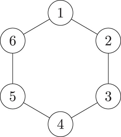
A cycle graph with six vertices.
Two-dimensional lattice graph. Consider an undirected graph
Figure 4 depicts two subgraphs of
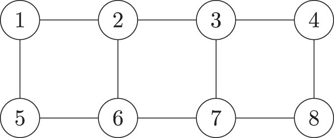
A two-dimensional lattice graph:
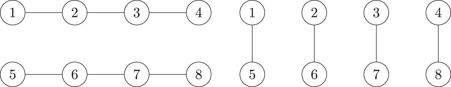
Subgraphs of
2.3 Moran’s
I
in matrix form
In this subsection, we represent Moran’s
where
3 Main results
In this section, we present the main results of the article.
Proposition 1
Denote Moran’s I for the case in which
Then, it follows that
Proof
See Appendix A.□
We make three remarks on Proposition 1.
The perspective on the four autocorrelation measures in different fields provided by Proposition 1 is beneficial because studying the properties of Moran’s
Proposition 1(ii) is of particular interest. This is because it is an example showing that time series analysis can be seen as a kind of spatial analysis. See also [14,15] for more such examples.
Let
4 Concluding remarks
In this article, using notions from linear algebraic graph theory, we have provided a unified perspective on some autocorrelation measures in different fields, namely, Orcutt’s first serial correlation coefficient,
Acknowledgments
The author would like to thank Kazuhiko Hayakawa, Ryo Okui, and four anonymous referees for their valuable comments on an earlier version of this article. The usual caveat applies.
-
Funding information: The Japan Society for the Promotion of Science supported this work through KAKENHI Grant No. 20K20759.
-
Ethical approval: The conducted research is not related to either human or animal use.
-
Conflict of interest: The author states no conflict of interest.
Appendix A Proof of Proposition 1
In this section, we provide the proof of Proposition 1. Let
A.1 Proof of Proposition 1(i):
ψ
=
I
c
Let
Next, given
which leads to
A.2 Proof of Proposition 1(ii):
ϕ
=
I
p
Let
Let
which leads to
A.3 Proof of Proposition 1(iii):
r
11
=
I
g
Denote the adjacency matrix of
Thus, given that
Accordingly, we prove them in order. First, given that
References
[1] G. H. Orcutt and J. O. Irwin, A study of the autoregressive nature of the time series used for Tinbergen’s model of the economic system of the United States 1919–1932, J. R. Stat. Soc. Ser. B. Stat. Methodol. 10 (1948), no. 1, 1–45, DOI: https://www.jstor.org/stable/2983795. 10.1111/j.2517-6161.1948.tb00001.xSearch in Google Scholar
[2] R. L. Anderson, Distribution of the serial correlation coefficient, Ann. Math. Stat. 13 (1942), no. 1, 1–13, DOI: https://doi.org/10.1214/aoms/1177731638. 10.1214/aoms/1177731638Search in Google Scholar
[3] E. J. Hannan, Time Series Analysis, Methuen, London, 1960. Search in Google Scholar
[4] P. A. P. Moran, Notes on continuous stochastic phenomena, Biometrika 37 (1950), no. 1/2, 17–23, DOI: https://doi.org/10.2307/2332142. 10.1093/biomet/37.1-2.17Search in Google Scholar
[5] A. D. Cliff and K. Ord, Spatial autocorrelation: A review of existing and new measures with applications, Econ. Geogr. 46 (1970), 269–292, DOI: https://doi.org/10.2307/143144. 10.2307/143144Search in Google Scholar
[6] A. D. Cliff and J. K. Ord, Spatial Autocorrelation, Pion, London, 1973. 10.2307/2529248Search in Google Scholar
[7] A. D. Cliff and J. K. Ord, Spatial Processes: Models and Applications, Pion, London, 1981. Search in Google Scholar
[8] A. Getis, A history of the concept of spatial autocorrelation: A geographer’s perspective, Geogr. Anal. 40 (2008), no. 3, 297–309, DOI: https://doi.org/10.1111/j.1538-4632.2008.00727.x.10.1111/j.1538-4632.2008.00727.xSearch in Google Scholar
[9] R. B. Bapat, Graphs and Matrices, second edition, Springer, London, 2014. 10.1007/978-1-4471-6569-9Search in Google Scholar
[10] E. Estrada and P. Knight, A First Course in Network Theory, Oxford University Press, Oxford, 2015. Search in Google Scholar
[11] J. Gallier, Spectral Theory of Unsigned and Signed Graphs. Applications to Graph Clustering: A Survey, 2016, https://arxiv.org/abs/1601.04692.Search in Google Scholar
[12] S. Dray, A new perspective about Moran’s coefficient: Spatial autocorrelation as a linear regression problem, Geogr. Anal. 43 (2011), no. 2, 127–141, DOI: https://doi.org/10.1111/j.1538-4632.2011.00811.x. 10.1111/j.1538-4632.2011.00811.xSearch in Google Scholar
[13] P. de Jong, C. Sprenger, and F. van Veen, On extreme values of Moran’s I and Geary’s c, Geogr. Anal. 16 (1984), no. 1, 17–24, DOI: https://doi.org/10.1111/j.1538-4632.1984.tb00797.x. 10.1111/j.1538-4632.1984.tb00797.xSearch in Google Scholar
[14] H. Yamada, A smoothing method that looks like the Hodrick-Prescott filter, Economet. Theor. 36 (2020), no. 5, 961–981, DOI: https://doi.org/10.1017/S0266466619000379. 10.1017/S0266466619000379Search in Google Scholar
[15] H. Yamada, Geary’s c and spectral graph theory, Mathematics 9 (2021), no. 19, 2465, DOI: https://doi.org/10.3390/math9192465. 10.3390/math9192465Search in Google Scholar
© 2023 the author(s), published by De Gruyter
This work is licensed under the Creative Commons Attribution 4.0 International License.
Articles in the same Issue
- Special Issue on Future Directions of Further Developments in Mathematics
- What will the mathematics of tomorrow look like?
- On H 2-solutions for a Camassa-Holm type equation
- Classical solutions to Cauchy problems for parabolic–elliptic systems of Keller-Segel type
- Control of multi-agent systems: Results, open problems, and applications
- Logical perspectives on the foundations of probability
- Subharmonic solutions for a class of predator-prey models with degenerate weights in periodic environments
- A non-smooth Brezis-Oswald uniqueness result
- Luenberger compensator theory for heat-Kelvin-Voigt-damped-structure interaction models with interface/boundary feedback controls
- Special Issue on Fractional Problems with Variable-Order or Variable Exponents (Part II)
- Positive solution for a nonlocal problem with strong singular nonlinearity
- Analysis of solutions for the fractional differential equation with Hadamard-type
- Hilfer proportional nonlocal fractional integro-multipoint boundary value problems
- A comprehensive review on fractional-order optimal control problem and its solution
- The θ-derivative as unifying framework of a class of derivatives
- Review Articles
- On the use of L-functionals in regression models
- Minimal-time problems for linear control systems on homogeneous spaces of low-dimensional solvable nonnilpotent Lie groups
- Regular Articles
- Existence and multiplicity of solutions for a new p(x)-Kirchhoff problem with variable exponents
- An extension of the Hermite-Hadamard inequality for a power of a convex function
- Existence and multiplicity of solutions for a fourth-order differential system with instantaneous and non-instantaneous impulses
- Relay fusion frames in Banach spaces
- Refined ratio monotonicity of the coordinator polynomials of the root lattice of type Bn
- On the uniqueness of limit cycles for generalized Liénard systems
- A derivative-Hilbert operator acting on Dirichlet spaces
- Scheduling equal-length jobs with arbitrary sizes on uniform parallel batch machines
- Solutions to a modified gauged Schrödinger equation with Choquard type nonlinearity
- A symbolic approach to multiple Hurwitz zeta values at non-positive integers
- Some results on the value distribution of differential polynomials
- Lucas non-Wieferich primes in arithmetic progressions and the abc conjecture
- Scattering properties of Sturm-Liouville equations with sign-alternating weight and transmission condition at turning point
- Some results for a p(x)-Kirchhoff type variation-inequality problems in non-divergence form
- Homotopy cartesian squares in extriangulated categories
- A unified perspective on some autocorrelation measures in different fields: A note
- Total Roman domination on the digraphs
- Well-posedness for bilevel vector equilibrium problems with variable domination structures
- Binet's second formula, Hermite's generalization, and two related identities
- Non-solid cone b-metric spaces over Banach algebras and fixed point results of contractions with vector-valued coefficients
- Multidimensional sampling-Kantorovich operators in BV-spaces
- A self-adaptive inertial extragradient method for a class of split pseudomonotone variational inequality problems
- Convergence properties for coordinatewise asymptotically negatively associated random vectors in Hilbert space
- Relating the super domination and 2-domination numbers in cactus graphs
- Compatibility of the method of brackets with classical integration rules
- On the inverse Collatz-Sinogowitz irregularity problem
- Positive solutions for boundary value problems of a class of second-order differential equation system
- Global analysis and control for a vector-borne epidemic model with multi-edge infection on complex networks
- Nonexistence of global solutions to Klein-Gordon equations with variable coefficients power-type nonlinearities
- On 2r-ideals in commutative rings with zero-divisors
- A comparison of some confidence intervals for a binomial proportion based on a shrinkage estimator
- The construction of nuclei for normal constituents of Bπ-characters
- Weak solution of non-Newtonian polytropic variational inequality in fresh agricultural product supply chain problem
- Mean square exponential stability of stochastic function differential equations in the G-framework
- Commutators of Hardy-Littlewood operators on p-adic function spaces with variable exponents
- Solitons for the coupled matrix nonlinear Schrödinger-type equations and the related Schrödinger flow
- The dual index and dual core generalized inverse
- Study on Birkhoff orthogonality and symmetry of matrix operators
- Uniqueness theorems of the Hahn difference operator of entire function with a Picard exceptional value
- Estimates for certain class of rough generalized Marcinkiewicz functions along submanifolds
- On semigroups of transformations that preserve a double direction equivalence
- Positive solutions for discrete Minkowski curvature systems of the Lane-Emden type
- A multigrid discretization scheme based on the shifted inverse iteration for the Steklov eigenvalue problem in inverse scattering
- Existence and nonexistence of solutions for elliptic problems with multiple critical exponents
- Interpolation inequalities in generalized Orlicz-Sobolev spaces and applications
- General Randić indices of a graph and its line graph
- On functional reproducing kernels
- On the Waring-Goldbach problem for two squares and four cubes
- Singular moduli of rth Roots of modular functions
- Classification of self-adjoint domains of odd-order differential operators with matrix theory
- On the convergence, stability and data dependence results of the JK iteration process in Banach spaces
- Hardy spaces associated with some anisotropic mixed-norm Herz spaces and their applications
- Remarks on hyponormal Toeplitz operators with nonharmonic symbols
- Complete decomposition of the generalized quaternion groups
- Injective and coherent endomorphism rings relative to some matrices
- Finite spectrum of fourth-order boundary value problems with boundary and transmission conditions dependent on the spectral parameter
- Continued fractions related to a group of linear fractional transformations
- Multiplicity of solutions for a class of critical Schrödinger-Poisson systems on the Heisenberg group
- Approximate controllability for a stochastic elastic system with structural damping and infinite delay
- On extremal cacti with respect to the first degree-based entropy
- Compression with wildcards: All exact or all minimal hitting sets
- Existence and multiplicity of solutions for a class of p-Kirchhoff-type equation RN
- Geometric classifications of k-almost Ricci solitons admitting paracontact metrices
- Positive periodic solutions for discrete time-delay hematopoiesis model with impulses
- On Hermite-Hadamard-type inequalities for systems of partial differential inequalities in the plane
- Existence of solutions for semilinear retarded equations with non-instantaneous impulses, non-local conditions, and infinite delay
- On the quadratic residues and their distribution properties
- On average theta functions of certain quadratic forms as sums of Eisenstein series
- Connected component of positive solutions for one-dimensional p-Laplacian problem with a singular weight
- Some identities of degenerate harmonic and degenerate hyperharmonic numbers arising from umbral calculus
- Mean ergodic theorems for a sequence of nonexpansive mappings in complete CAT(0) spaces and its applications
- On some spaces via topological ideals
- Linear maps preserving equivalence or asymptotic equivalence on Banach space
- Well-posedness and stability analysis for Timoshenko beam system with Coleman-Gurtin's and Gurtin-Pipkin's thermal laws
- On a class of stochastic differential equations driven by the generalized stochastic mixed variational inequalities
- Entire solutions of two certain Fermat-type ordinary differential equations
- Generalized Lie n-derivations on arbitrary triangular algebras
- Markov decision processes approximation with coupled dynamics via Markov deterministic control systems
- Notes on pseudodifferential operators commutators and Lipschitz functions
- On Graham partitions twisted by the Legendre symbol
- Strong limit of processes constructed from a renewal process
- Construction of analytical solutions to systems of two stochastic differential equations
- Two-distance vertex-distinguishing index of sparse graphs
- Regularity and abundance on semigroups of partial transformations with invariant set
- Liouville theorems for Kirchhoff-type parabolic equations and system on the Heisenberg group
- Spin(8,C)-Higgs pairs over a compact Riemann surface
- Properties of locally semi-compact Ir-topological groups
- Transcendental entire solutions of several complex product-type nonlinear partial differential equations in ℂ2
- Ordering stability of Nash equilibria for a class of differential games
- A new reverse half-discrete Hilbert-type inequality with one partial sum involving one derivative function of higher order
- About a dubious proof of a correct result about closed Newton Cotes error formulas
- Ricci ϕ-invariance on almost cosymplectic three-manifolds
- Schur-power convexity of integral mean for convex functions on the coordinates
- A characterization of a ∼ admissible congruence on a weakly type B semigroup
- On Bohr's inequality for special subclasses of stable starlike harmonic mappings
- Properties of meromorphic solutions of first-order differential-difference equations
- A double-phase eigenvalue problem with large exponents
- On the number of perfect matchings in random polygonal chains
- Evolutoids and pedaloids of frontals on timelike surfaces
- A series expansion of a logarithmic expression and a decreasing property of the ratio of two logarithmic expressions containing cosine
- The 𝔪-WG° inverse in the Minkowski space
- Stability result for Lord Shulman swelling porous thermo-elastic soils with distributed delay term
- Approximate solvability method for nonlocal impulsive evolution equation
- Construction of a functional by a given second-order Ito stochastic equation
- Global well-posedness of initial-boundary value problem of fifth-order KdV equation posed on finite interval
- On pomonoid of partial transformations of a poset
- New fractional integral inequalities via Euler's beta function
- An efficient Legendre-Galerkin approximation for the fourth-order equation with singular potential and SSP boundary condition
- Eigenfunctions in Finsler Gaussian solitons
- On a blow-up criterion for solution of 3D fractional Navier-Stokes-Coriolis equations in Lei-Lin-Gevrey spaces
- Some estimates for commutators of sharp maximal function on the p-adic Lebesgue spaces
- A preconditioned iterative method for coupled fractional partial differential equation in European option pricing
- A digital Jordan surface theorem with respect to a graph connectedness
- A quasi-boundary value regularization method for the spherically symmetric backward heat conduction problem
- The structure fault tolerance of burnt pancake networks
- Average value of the divisor class numbers of real cubic function fields
- Uniqueness of exponential polynomials
- An application of Hayashi's inequality in numerical integration