Wave propagation in functionally graded piezoelectric-piezomagnetic rectangular bars
-
Bo Zhang
 ,
Abid A. Shah
,
Abid A. Shah

Abstract
In recent years, guided wave propagation in piezoelectric-piezomagnetic composite (PPC) structures are paid much attention for the design and optimization of PPC transducers. Previous investigations are mainly limited in horizontally infinite flat plates, axially infinite hollow cylinders, and so on. They are all one-dimensional model structures, i.e. structures having variable displacement field in only one direction, and the other two displacement fields are both constant. In this paper, a double orthogonal polynomial series approach is proposed to solve the guided wave in two-dimensional model structures, namely, a functionally graded piezoelectric-piezomagnetic (FGPP) bar with a rectangular cross section. The validity of the double polynomial approach is illustrated by the comparison with the available reference results for a pure elastic homogeneous rectangular bar. The guided wave characteristics, including dispersion curves and mechanical displacement distributions, are discussed by calculating various FGPP rectangular bars.
1 Introduction
In recent years, with the increasing usage in sensors, actuators, and storage devices [1], [2], [3], piezoelectric-piezomagnetic composites (PPCs) have received considerable research effort. Wave propagation in various PPC also attracted many researchers for the purpose of design and optimization of PPC transducers.
The effectively axial shear wave velocity and attenuation factor of PPCs were obtained by Chen and Shen [4]. By using “bar model”, Wei and Su [5] studied the axisymmetric flexural wave in piezoelectric-piezomagnetic cylinders. Chen and Chen [6] investigated the Love wave behavior in magneto-electro-elastic multilayered structures by the propagation matrix method. Resorting to the propagator matrix and state-vector (or state space) approaches, Chen et al. [7] presented the propagation of harmonic waves in magneto-electro-elastic multilayered plates. Yu et al. [8] investigated the guided wave in inhomogeneous magneto-electro-elastic hollow cylinders and spherical curved plates [9] by virtue of the Legendre orthogonal polynomial series expansion approach.
Some special wave problems in PPC structures also attracted attention. Wave propagation band gaps in piezoelectric-piezomagnetic periodically layered structures are investigated [10], [11], [12]. The penetration depth of the Bleustein-Gulyaev waves in a functionally graded magneto-electro-elastic half-space is discussed by Li et al. [13]. SH waves propagating in piezoelectric-piezomagnetic layered structures with imperfect interfaces are investigated by Sun et al. [14] and Nie et al. [15]. The reflection and transmission of plane waves at an imperfectly bonded interface between piezoelectric-piezomagnetic media are discussed by Pang and Liu [16]. Xue et al. [17] investigated the solitary waves in a magneto-electro-elastic circular bar by virtue of the Jacobi elliptic function expansion method. By using Legendre and Laguerre polynomial approach, Matar et al. [18] modeled the wave propagation in layered magneto-electro-elastic media. The influences of the gradient factor on the longitudinal wave along a functionally graded magneto-electro-elastic bar are discussed by Xue and Pan [19]. The influences of initial stresses on Rayleigh wave in a magneto-electro-elastic half-space are studied by Zhang et al. [20].
As can be seen from the previously mentioned simple review, wave motions in many magneto-electro-elastic structures have been studied. However, these structures are all semi-infinite structures and one-dimensional (1-D) model structures, i.e. structures having variable displacement field in only one direction, and the other two displacement fields are both constant, such as horizontally infinite flat plates and axially infinite hollow cylinders. In practical applications, many sensitive elements have very limited finite dimension in two directions. One-dimensional models are not suitable for these structures. This paper proposes a double orthogonal polynomial series approach to solve wave propagation in a two-dimensional (2-D) model structure: functionally graded piezoelectric-piezomagnetic (FGPP) bar with rectangular cross section. The dispersion curves and the mechanical displacement profiles of various FGPP rectangular bars are presented and discussed. In this paper, the open circuit is assumed.
2 Mathematics and formulation of the problem
We consider an orthotropic magneto-electro-elastic rectangular bar, which is infinite in wave propagating direction and is polarized in z direction. Its width is d and its height is h, as shown in Figure 1. The origin of the Cartesian coordinate system is located at a corner of the rectangular cross section, and the bar lies in the positive y-z region, where the cross section is defined by the region 0≤z≤h and 0≤y≤d.

Schematic diagram of a bar with rectangular cross section.
For the wave propagation problem considered in this paper, body forces and electric charges are assumed to be zero. Thus, the dynamic equations for the rectangular bar are governed by
where Tij, ui, Di, and Bi are the stress, elastic displacement, electric displacement, and magnetic induction components, respectively, and ρ is the density of the material.
In this paper, electric and magnetic fields are assumed conservative. The relationships between the general strain and the general displacement components can be expressed as
where εij, Ei, and Hi are the strain, electric field, and magnetic field, respectively, and ϕ and Ψ are the electric potential and magnetic potential components, respectively.
We introduce the function I(y, z) as follows:
where π(y) and π(z) are rectangular window functions
where Cij, eij, and qij are the elastic, piezoelectric, and piezomagnetic coefficients, respectively, and ∈ij, gij, and μij are the dielectric, magnetoelectric, and magnetic permeability coefficients, respectively.
For the FGPP bar of material properties varying in the z-direction (we call it z-directional FGPP bar; the undermentioned FGPP bars are all z-directional FGPP bars unless otherwise specified), the elastic parameters of the bar are functions of z, which can be expressed as
With implicit summation over repeated indices, Cij(z) can be written compactly as
Similarly, the other material coefficients can be represented by
For the FGPP bar of material properties varying in the y-direction (we call it y-directional FGPP bar), the material parameters of the bar are functions of y, which can be expressed as
For plane time-harmonic wave propagating in the x-direction of a rectangular bar, we assume the displacement, electric potential, and magnetic potential components having the following form:
where U(y, z), V(y, z), and W(y, z) represent the mechanical displacement amplitudes in the x-, y-, and z-directions, respectively, and X(y, z) and Y(y, z) represent the amplitudes of electric potential and magnetic potential. k is the magnitude of the wave vector in the propagation direction, and ω is the angular frequency.
Substituting Equations (2)–(5) or (6), and (7) into Equation (1), the governing differential equations in terms of displacement, electric potential, and magnetic potential components can be obtained. Here, the case that the material gradient direction and the polarizing direction are the same is given as follows:
where the subscript comma indicates partial derivative.
To solve the coupled wave Equation (8), U(y, z), V(y,z), W(y, z), X(y, z), and y(y, z) are all expanded into products of two Legendre orthogonal polynomial series
where
with Pm and Pj being the mth and the jth Legendre polynomials. Theoretically, m and j run from 0 to ∞. However, in practice, the summation over the polynomials in Equation (9) can be truncated at some finite values m=M and j=J, when the effects of higher order terms become negligible.
Equation (8) is multiplied by Qn(z) with n running from 0 to M, and by Qp(y) with p from 0 to J, respectively. Then integrating over z from 0 to h and over y from 0 to d gives the following system of linear algebraic equations:
where
Equation (11e) can be written as follows:
Substituting Equation (12) into Equation (11d),
Substituting Equation (13) into Equation (12),
Substituting Equations (13) and (14) into Equations (11a), (11b), and (11c),
where
So, Equation (15) forms the eigenvalue problem to be solved. To solve it, we first give a set of real k. Then we determine the eigenvalues and eigenvectors of -M-1A̅ for each given k. The eigenvalue ω2 gives the angular frequency of the guided wave, the eigenvectors
3 Numerical results and discussion
The Voigt-type model is used in this study to calculate the effective parameters of the FGPP bar, which can be expressed as follows:
where Vi(z) and Ci denote the volume fraction of the ith material and the corresponding physical property of the ith material, respectively, and ∑Vi(z)=1. Thus, the properties of the FGPP can be expressed as follows:
for z-directional FGPP rectangular bar,
for y-directional FGPP rectangular bar,
According to Equations (5) and (6), the gradient profile of the material volume fraction can be expressed as a power series expansion. The coefficients of the power series can be determined using the Mathematica function “Fit”.
On the basis of the mathematical formulation as presented in Section 2, computer programs in terms of the double polynomial method have been written using the software Mathematica 5.0 (Wolfram Research) to calculate the dispersion curves and the mechanical displacement distributions for the FGPP rectangular bars.
3.1 Comparison with the available solution
Because no reference results for the guided waves in FGPP or FG rectangular rings can be found in literature, we consider a homogeneous square steel bar with CL=5.85 km/s, CT=3.23 km/s, and h=d=5.08 mm to make a comparison with known results from the semi-analytical finite element method [22]. Here, CL and CT are the longitudinal and transversal wave velocities, respectively. Figure 2 shows the corresponding dispersion curves, where dotted lines are from Hayashi et al. [22] and solid lines are obtained from the present polynomial approach. As can be seen, the results from the double polynomial approach agree well with the reference data, which verify the correctness and the accuracy of the present method.
![Figure 2: Phase velocity dispersion curves for the steel square bar; dotted lines: results from the semi-analytical finite element method [22]; solid lines: the authors’ results.](/document/doi/10.1515/secm-2014-0082/asset/graphic/j_secm-2014-0082_fig_002.jpg)
Phase velocity dispersion curves for the steel square bar; dotted lines: results from the semi-analytical finite element method [22]; solid lines: the authors’ results.
3.2 Dispersion curves in FGPP rectangular bars
In this section, we take the Ba2TiO3-CoFe2O4 FGPP rectangular bars (the bottom surface is pure Ba2TiO3) as examples to discuss the wave characteristics. Their corresponding material parameters are given in Table 1. First, we consider two z-directional FGPP square bars. Their gradient functions are as follows: bar a, linearly FGPP bar [V1(z)=z/h], and bar b, cubically FGPP bar [(V1(z)=(z/h)3]. Their velocity dispersion curves are shown in Figure 3. It can be seen that the first four wave modes have no cutoff frequencies. This feature is different from that of an infinite FGPP flat plate, in which the first three modes have no cutoff frequencies. Furthermore, different gradient varieties result in different dispersive characteristics. The wave speed of linearly graded bar is a little higher than that of cubically graded bar because the volume fraction of Ba2TiO3 in linearly graded bar is less than that in cubically graded bar, and the bulk wave speed of Ba2TiO3 is lower than that of CoFe2O4.
Physical parameters of the two materials with polarization in the thickness direction.
| Property | C11 | C12 | C13 | C22 | C23 | C33 | C44 | C55 | C66 |
|---|---|---|---|---|---|---|---|---|---|
| Ba2TiO3 | 166 | 77 | 78 | 166 | 78 | 162 | 43 | 43 | 44.6 |
| CoFe2O4 | 286 | 173 | 170.5 | 286 | 170.5 | 269.5 | 45.3 | 45.3 | 56.5 |
| e15 | e24 | e31 | e32 | e33 | ∈11 | ∈22 | ∈33 | ρ | |
| Ba2TiO3 | 11.6 | 11.6 | -4.4 | -4.4 | 18.6 | 112 | 112 | 126 | 5.8 |
| CoFe2O4 | 0 | 0 | 0 | 0 | 0 | 0.8 | 0.8 | 0.93 | 5.3 |
| q15 | q24 | q31 | q32 | q33 | μ11 | μ22 | μ33 | ||
| Ba2TiO3 | 0 | 0 | 0 | 0 | 0 | 5 | 5 | 10 | |
| CoFe2O4 | 550 | 550 | 580.3 | 580.3 | 699.7 | -590 | -590 | 157 |
Units: Cij (109 N/m2), ∈ij (10-10 F/m2), eij (C/m), qij (N/Am), μij (10-6 Ns2/C2), ρ (103 kg/m3).

Phase velocity dispersion curves for two z-directional FGPP square bars: (A) linearly graded bar and (B) cubically graded bar.
Then two linearly FGPP rectangular bars are considered. They are bar c, z-directional FGPP bar with d/h=2, and bar, d y-directional [V1(y)=y/d] FGPP bar with d/h=0.5. Their dispersion curves are shown in Figure 4. It can be seen that there is just a little difference between Figures 4A and B. However, Figures 3A and 4A have obvious differences. In fact, if bar c was rotated 90°, it would have the same volume fraction and the same width-to-thickness ratio as bar d. The difference between bars c and d is just their different polarizations. For bar c, its polarization is identical to its gradient direction, whereas for bar d, its polarization is vertical to its gradient direction. By contrast, bars c and a just have different width-to-thickness ratios. Thus, we can think that the gradient variation and the width-to-thickness ratio have significant influences on the dispersion curves, but gradient direction just has a weak influence.

Phase velocity dispersion curves for two linearly FGPP rectangular bars: (A) z-directional with d/h=2 and (B) y-directional with d/h=0.5.
3.3 Displacement shapes
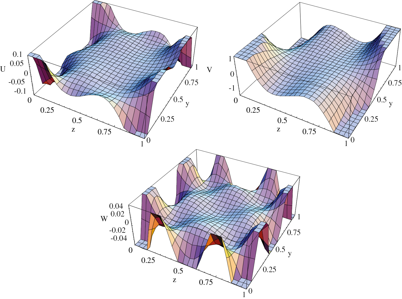
First, Figures 5 and 6 show the displacement shapes of the first and fourth modes for bar a. It can be seen that the displacements mostly distribute around the bottom side. Then the displacement shapes of the first and fourth modes for another bar, bar e: z-directional sinusoidally [V1(z)=sin(πz)] FGPP square bar, is shown in Figures 7 and 8. This time, the displacements mostly distribute around the bottom and the top sides but few distribute around the middle of bar e. Thus, we can think the high-frequency wave displacements always distribute around the side with more Ba2TiO3. In the displacement figures, when the amplitudes around the corners are too high compared with the other positions, they are truncated. Thus, the displacement amplitudes seem to be plateaus around the corners. Otherwise, the amplitude variations of other positions cannot be shown clearly.

Displacement shapes of the first mode for the linearly FGPP square bar at kd=90.1.

Displacement shapes of the fourth mode for the linearly FGPP square bar at kd=90.1.

Displacement shapes of the first mode for the sinusoidally FGPP square bar at kd=90.1.
Displacement shapes of the fourth mode for the sinusoidally FGPP square bar at kd=90.1.
From Figures 7 and 8, we can notice another phenomenon: the displacements of the sinusoidally FGPP bar are always symmetric or antisymmetric with respect to both y- and z-axes because the sinusoidally FGPP bar is symmetric both on geometry and on material distribution. By contrast, the material distribution of bar a is just symmetric with respect to y-axis. As can be seen in Figures 5 and 6, the displacements of the linearly FGPP bar are always symmetric or antisymmetric with respect to y-axis but not to z-axis.
4 Conclusions
In this paper, a double orthogonal polynomial series approach is proposed to solve the wave propagation analysis of a 2-D FGPP rectangular bar. The dispersion curves and the displacement distributions of various FGPP rectangular bars are presented and discussed. According to the numerical results, we can draw the following conclusions:
Numerical comparison of the dispersion curves with reference solutions shows that the double orthogonal polynomial method is appropriate to solve the guided wave propagation problem in 2-D FGPP structures.
Both the width-to-height ratio and the gradient function have significant influences on the guided wave characteristics, but gradient direction just has a weak influence.
High-frequency waves propagate predominantly around the side with more materials having lower wave speed.
Acknowledgments
This work was supported by the Outstanding Youth Science Foundation of Science and Technology Agency of Henan Province (grant no. 144100510016) and the Special Items of Basic Scientific Research Business of Henan Polytechnic University (grant no. NSFRF140301).
References
[1] Achenbach JD. Int. J. Sol. Struct. 2000, 37, 13–27.10.1016/S0020-7683(99)00074-8Search in Google Scholar
[2] Buchanan GR. Comparison of Effective Moduli for Multiphase Magneto-Electro-Elastic Materials. Proceedings of the Tenth International Conference on Composite/Nano Engineering, New Orleans, 2003.Search in Google Scholar
[3] Tiercelin N, Dusch Y, Preobrazhensky V, Pernod P. J. Appl. Phys. 2011, 109(7), 07D726-07D726-3.10.1063/1.3559532Search in Google Scholar
[4] Chen P, Shen Y. Int. J. Sol. Struct., 2007, 44, 1511–1532.10.1016/j.ijsolstr.2006.06.037Search in Google Scholar
[5] Wei J, Su XY. AcLa ScienLiarum NaLuralium LniversiLaLis Pekinensis, 2006, 42, 310–314 (in Chinese).Search in Google Scholar
[6] Chen JY, Chen HL. Acta Materiae Compositae Sinica, 2006, 23, 181–184 (in Chinese).10.17660/ActaHortic.2006.720.17Search in Google Scholar
[7] Chen JY, Pan E, Chen HL. Int. J. Sol. Struct. 2007, 44, 1073–1085.10.1016/j.ijsolstr.2006.06.003Search in Google Scholar
[8] Yu JG, Ma QJ, Su S. Ultrasonics, 2008, 48, 664–677.10.1016/j.ultras.2008.03.005Search in Google Scholar
[9] Yu JG, Ma QJ. Mech. Adv. Mater. Struct. 2010, 17, 287–301.10.1080/15376490903556642Search in Google Scholar
[10] Liu J, Wei W, Fang D. Acta Mech. Solida Sin. 2010, 23, 77–84.10.1016/S0894-9166(10)60009-2Search in Google Scholar
[11] Pang Y, Wang YS, Liu JX, Fang DN. Smart Mater. Struct. 2010, 19, 055012.10.1088/0964-1726/19/5/055012Search in Google Scholar
[12] Zhao J, Zhong Z, Pan Y. J. Acoust. Soc. Am. 2012, 131, 3327–3327.10.1121/1.4708451Search in Google Scholar
[13] Li P, Jin F, Qian Z. Eur. J. Mech. A. Solids. 2013, 37, 17–23.10.1016/j.euromechsol.2012.04.004Search in Google Scholar
[14] Sun WH, Ju GL, Pan JW, Li YD. Ultrasonics. 2011, 51, 831–838.10.1016/j.ultras.2011.04.002Search in Google Scholar
[15] Nie G, Liu J, Fang X, An Z. Acta Mech. 2012, 223, 1999–2009.10.1007/s00707-012-0680-6Search in Google Scholar
[16] Pang Y, Liu JX. Eur. J. Mech. A. Solids. 2011, 30, 731–740.10.1016/j.euromechsol.2011.03.008Search in Google Scholar
[17] Xue CX, Pan E, Zhang SY. Smart Mater. Struct. 2011, 20, 105010.10.1088/0964-1726/20/10/105010Search in Google Scholar
[18] Matar OB, Gasmi N, Zhou H, Goueygou M, Talbi A. J. Acoust. Soc. Am. 2013, 133: 1415.10.1121/1.4776198Search in Google Scholar
[19] Xue CX, Pan E. Int. J. Eng. Sci. 2013, 62, 48–55.10.1016/j.ijengsci.2012.08.004Search in Google Scholar
[20] Zhang R, Pang Y, Feng W. Mech. Adv. Mater. Struct. 2014, 21, 538–543.10.1080/15376494.2012.699595Search in Google Scholar
[21] Datta S, Hunsinger BJ. J. Appl. Phys. 1978, 49, 475–479.10.1063/1.324670Search in Google Scholar
[22] Hayashi T, Song W-J, Rose JL. Ultrasonics. 2003, 41, 175–183.10.1016/S0041-624X(03)00097-0Search in Google Scholar
©2017 Walter de Gruyter GmbH, Berlin/Boston
This article is distributed under the terms of the Creative Commons Attribution Non-Commercial License, which permits unrestricted non-commercial use, distribution, and reproduction in any medium, provided the original work is properly cited.
Articles in the same Issue
- Frontmatter
- Original articles
- Wave propagation in functionally graded piezoelectric-piezomagnetic rectangular bars
- Graphene/poly(vinylidene fluoride) dielectric composites with polydopamine as interface layers
- A novel biaxial double-negative metamaterial for electromagnetic rectangular cloaking operation
- Formation of homogenous copper film on MWCNTs by an efficient electroless deposition process
- Nano-SiCp/Al2014 composites with high strength and good ductility
- Microstrip line-fed monopole antenna on an epoxy-resin-reinforced woven-glass material for super wideband applications
- Influence of casting speed on fabricating Al-1%Mn and Al-10%Si alloy clad slab
- Thermal insulating epoxy composite coatings containing sepiolite/hollow glass microspheres as binary fillers: morphology, simulation and application
- Analysis of influence of fibre type and orientation on dynamic properties of polymer laminates for evaluation of their damping and self-heating
- Dynamic stability of nanocomposite viscoelastic cylindrical shells coating with a piezomagnetic layer conveying pulsating fluid flow
- Buckling and layer failure of composite laminated cylinders subjected to hydrostatic pressure
- One-step preparation and characterization of core-shell SiO2/Ag composite spheres by pulse plating
- The failure mechanism of carbon fiber-reinforced composites under longitudinal compression considering the interface
- A thermal-plastic model of friction stir welding in aluminum alloy
- A model for longitudinal tensile strength prediction of low braiding angle three-dimensional and four-directional composites
- Nonlinear stability of shear deformable eccentrically stiffened functionally graded plates on elastic foundations with temperature-dependent properties
- Design and multibody dynamics analyses of the novel force-bearing structures for variable configuration spacecraft