Algebraic and qualitative remarks about the family yy′ = (αxm+k–1 + βxm–k–1)y + γx2m–2k–1
-
Jorge Rodríguez-Contreras


Abstract
The aim of this paper is the analysis, from algebraic point of view and singularities studies, of the 5-parametric family of differential equations
where a, b, c ∈ ℂ, m, k ∈ ℤ and
This family is very important because include Van Der Pol equation. Moreover, this family seems to appear as exercise in the celebrated book of Polyanin and Zaitsev. Unfortunately, the exercise presented a typo which does not allow to solve correctly it. We present the corrected exercise, which corresponds to the title of this paper. We solve the exercise and afterwards we make algebraic and of singularities studies to this family of differential equations.
Introduction
Dynamical systems is a topic of interest for a large number of theoretical physicist and mathematicians due to the seminal works of H. Poincaré. It is well known that any dynamical system is a system which evolves in the time. H. Poincaré introduced the qualitative approach to study dynamical systems, which has been useful to study theoretical aspects and applications to biology, chemistry, physics, among others, see [1, 2, 3, 4, 5, 6, 7].
On another hand, E. Picard and E. Vessiot introduced an algebraic approach to study linear differential equations based on the Galois theory for polynomials, see [8, 9, 10, 11, 12, 13]. Combination of dynamical systems with differential Galois theory is a recent topic which started with the works of J.J Morales-Ruiz (see [12] and references therein) and with the works of J.-A. Weil (see [14]). Further works about applications of differential Galois theory include [15, 16, 17].
The Handbook of Exact Solutions of Ordinary Differential Equations, see [18], is one important reference for scientists and engineers interested in solving explicitly ordinary differential equations. This book contains around 3, 000 nonlinear ordinary differential equations with solutions, as well as exact, symbolic, and numerical methods for solving nonlinear equations. Nonlinear equations and systems with first-, second-, third-, fourth-, and higher-order are considered there.
Inspired by a previous version of the paper [19], we analysed the Exercise 11 in [18, §1.3.3], which corresponds to a five parametric family of differential equations. We discovered a typo (also corrected by us), which was corrected in the final version of [19] to study from differential Galois Theory point of view the integrability of the dynamical system proposed in such excercise.
We call as Polyanin-Zaitsev vector field to the vector field associated to this system of differential equations that comes from the corrigendum of the Exercise 11 in [18, § 1.3.3]. Moreover, we study integrability aspects using differential Galois theory, following [9, 19] as well qualitative aspects due to the foliation associated to Polyanin-Zaitzev vector field is a Liénard equation, which is closely related to a Van Der Pol equation.
This paper not only present the corrigendum and complete solution of the Polyanin-Zaitsev excercise mentioned above, it also extends the results given in [19] concerning the Polyanin-Zaitsev vector field. From algebraic point of view we give conditions over the parameters to have polynomial vector field, moreover we obtain the critical points for some particular cases and we describe their behavior.
The results of this paper were obtained, but not published, during the seminar Algebraic Methods in Dynamical Systems in 2013 developed by the first author and in the master thesis of the second author in 2014 (supervised by the first and third author).
1 Preliminaries
In this section we provide the necessary theoretical background to understand the rest of the paper.
A planar polynomial system of degree n is given by
being P, Q ∈ ℂ[x, y] and n = max(deg P, deg Q). By X := (P, Q) we denote the polynomial vector field associated to the system (1). The planar polynomial vector field X can be also writen in the form
A foliation of a polynomial vector field of the form (1) is given by
Following [6], we present the following theorem, which allow us the characterization of the critical points.
Theorem 1.1
Let X, Y be analytic functions with polynomial part containing terms of degree greater than 1. Consider the planar differential system
being the origin an isolated critical point. Assume
as the solutions of y + X(x, y) = 0 near to (0, 0). Suppose
and also
Then the following statements hold:
If α is even and α > 2β + 1, then (0, 0) is a saddle node.
If α is even and α < 2β + 1 or Φ(x) ≡ 0, then the flow near of (0, 0) have two hyperbolic sectors.
If α is odd and a > 0, then (0, 0) is a saddle point.
If α is odd and a < 0, several cases can occur:
in this case for b < 0 the critical point (0, 0) is a stable node, while for b > 0 the critical point (0, 0) is unstable node.
in this case the flow near to the critical point (0, 0) is topologically conformed by an elliptic sector joint with an hyperbolic sector.
in this case the critical point (0, 0) is focus or center.
2 Corrigendum to the problem
The original Exercise 11, section 1.3.3 of the book of Polyanin-Zaitsev (see [18, § 1.3.3.11]) was presented as follows:
The transformation z = xk, y = xm(t + axk + bx–k) leads to a Riccati equation with respect to z = z(t):
The substitution
The transformation
where ν is a root of the quadratic equation
A typo in this exercise does not allows its solving. The correction of the problem is presented in the following proposition:
Proposition 2.1
Given the family of Liénard equations of the form:
the change of variables z = xk and y = xm(t + axk + bx–k) allow to transform any equation of this family to a Riccati equation.
Proof
The system of equations, associated with this Liénard equation is:
Now, applying the transformation
and differentiating we have that:
then, the associated foliation has the form ydy = (f(x)y – g(x))dx, being f(x) = (a(2m + k)xm+k–1 + b(2m – k)xm–k–1) and g(x) = (a2mx4k+cx2k+b2m)x2m–2k–1 as the Liénard equations. Now we compute each part of this equality, thus we obtain the left side as:
and the right side as
For our purpose, we organize the terms with respect to dz, that is:
Now organizing the terms again we have:
Thus, we obtain the Riccati equation:
and we conclude the proof.□
For the rest of transformations proposed in the Exercise of Polyanin-Zaitsev we need the results concerning the transformations, which will be given in the next section.
3 Some transformations
In this section we study some transformations that allow us to complete the exercise stated by Polyanin-Zaitsev above.
Lemma 3.1
If R = a1x2 + a1x + a0, S = b1x + b0, with a2, b1 ≠ 0. Then the differential equation
with y = y(x) is transformed in the equation
with
Proof
We divide all by
Now in R we complete the square
Then:
Assume
then
Replacing x in the polynomial S in term of τ, we get:
Then, if
Now, if
where ŷ = y(x(τ)), and the transformation
Remark 3.1
The differential equation of the form
with λ = n(n + 1 + ã + b̃) and n ∈ ℕ, is known as Jacobi equation (in general form). It is a particular case of the hypergeometric equation, but the solutions include Jacobi polynomials. If we take ã = b̃ and λ̃ = n(n + 2ã) with n ∈ ℕ, we get a Gegenbauer equation (or ultraspherical case):
Now we study a special transformation, in the following theorem:
Theorem 3.2
The differential equation
with ai ∈ ℂ(x), with an ≠ 0, can be transformed into the differential equation
with bi ∈ ℂ(x).
Proof
Following the Lemma 3.1 and taking the implicit transformation z = ε(t)y + μ(t) with ε(t), μ(t) ∈ ℂ(x), we compute the first equation applying the change of variable
Then, computing in general form the Leibniz rule we get:
Continuing of this form, we divide all equation by ε. Then, we use the same method of the indeterminate coefficients to calculate ε and the bi coefficient:
If we take y(n–1):
then:
From this differential equation we get an appropriate ε value, and with it we obtain the coefficient bi.
If we take y(n–2):
If we take y(n–3):
Continuing of this form we see, that for any k ∈ ℕ the recurrent formulae will be:
□
If in the previous theorem, we consider k̃ = 0, we get the next corollary:
Corollary 3.3
The differential equation
with ai ∈ ℂ(x) can be transformed in the following equation
where bi ∈ ℂ(x).
Example
Applying the transformation over the general second order differential equation z″ + a1z′ + a0z = 0:
Using Theorem 3.2, we get
In this way we arrive to
In the following theorem we recall that a Hamiltonian Change of Variable z = z(x) is a change of variable, where (z(x), z′(x)) is a solution curve of a Hamiltonian system of one degree of freedom. The new derivation is given by
Theorem 3.4
Let Q and L be as in (3.1), with a1 = b1 = 0 or
is transformed in the equation
Owing to λ = n(n + 1 + ã + b̃), we have the Jacobi equation with ã = b̃. Moreover, if λ = n(n + 2ã) then we obtain a Gegenbauer equation.
Proof
If we assume a1 = b0 = 0, we obtain
Now, by hypothesis ξ = ∂τ
thus
Furthermore, due to ξ = ∂τ
i.e
Now
We compute all elements of the Hamiltonian change of variable
If we replace, in the transformed differential equation, we obtain:
It is equivalent to Gegenbauer equation with
Finally if
If
i.e the initial differential equation will be:
for instance, the same differential equation of the previous case.□
Now we transform the Gegenbauer equation into an Hypergeometric equation.
Lemma 3.5
The Gegenbauer equation
is transformed into an hypergeometric equation
where a = μ – ν, b = ν + μ + 1, c = μ + 1 and
Proof
For this transformation we will use a Hamiltonian change of variable, over the independent variable of the Gegenbauer equation x = 1 – 2z. Then
Substituting in the Gegenbauer equation, we obtain
Thus, we obtain the equation
We know that Hypergeometric equation is of the form
Then, we compute the parameters values a, b and c as follows:
Therefore
which concludes the proof.□
Proposition 3.6
Through the Hamiltonian change of variables x = 1 – 2ξ and
into the Legendre equation
Proof
Firstly we transform the Legendre equation into the Hypergeometric equation:
If
and
Now dividing by
Now we obtain
Now applying the Hamiltonian change of variable
Following exactly the reversed process, we can transform a Hypergeometric equation into Legendre equation.□
Example
Transform the next equation on ultraespheric form.
Now R = mt2 + c0,
Applying the previous lemma we have the equation:
Now applying the previous theorem we get:
with û(ξ) = ŵ(τ(ξ)).
Remark 3.2
If we have our equation in the Legendre form, we apply the proposition 3.6 and therefore we can study it as in [19] to conclude the integrability or non-integrability, of the Liénard equation. Moreover, such as we will see in the next section, through equation (5) in Legendre’s form we can apply the Kimura table, see [19].
4 Polyanin-Zaitsev vector field
The associated system of the Polyanin-Zaitsev vector field, with a, b, c, m, k ∈ ℝ, is given by:
with α = a(2m + k), β = b(2m – k) and γ = (a2mx4k + cx2k + b2m), where the Polyanin-Zaitsev vector field is given by X =: (P, Q), being,
The next proposition can illustrate the cases in which the Polyanin-Saitsev vector field is formed by non trivial polynomial functions.
Proposition 4.1
The system (5) is a not null differential polynomial system if it is equivalently to one of the next families:
with s, p, r ∈ ℤ defined in the proof.
Proof
The system (5) is a polynomial system if Q is a polynomial function, that is, the exponents of each term must be non negative integer. Furthermore, we need to consider the values of the constants a, b and c. Now we consider the different possibilities for these constants:
For a ≠ 0, b ≠ 0, c ≠ 0, it must be satisfied:
being s, p, r ∈ ℤ+. Thus
For a = 0, b ≠ 0, c ≠ 0, the system (5) is reduced to:
since the exponents must be non-negative integers, then:
for instance, we arrive to the system:
For a ≠ 0, b ≠ 0, c = 0, the system (5) is reduced to:
again the exponents must be non-negative integers, therefore:
thus,
For a = 0, b = 0, c ≠ 0, the system (5) is reduced to:
due to the exponents must be non-negative integers, we arrive to 2m – 1 = r ∈ ℕ, that is,
For a ≠ 0, b = 0, c ≠ 0, the system (5) is reduced to:
in this case:
then
For a = 0, b ≠ 0, c = 0, the system (5) is reduced to:
in this case:
then there is a line of solutions, with r ∈ ℤ+.
In this case the associated family is:
For a ≠ 0, b = 0, c = 0, the system (5) is reduced to:
in this case:
then the associated family is:
□
5 Finite critical points
In this section, we present an study about the existence of finite critical points and the stability for each family associated to the Polyanin-Zaitsev vector field.
Proposition 5.1
For the vector field given by (5), with k ∈ ℤ the following statements holds:
If c2 – 4a2b2m2 < 0, or c2 – 4a2b2m2 ≥ 0 and c > 0, then (0, 0) is the only one finite critical point of the family.
If c2 – 4a2b2m2 = 0 and c < 0 then the system have three finite critical points.
If c2 – 4a2b2m2 ≥ 0, c < 0 and k ∈ ℤ then exist five finite critical points for the systems.
Proof
For this proof we take the family (6) as form (5). Then, we will have to solve the system:
If y = 0, then (a2mx4k + cx2k + b2m)x2m–2k–1 = 0, with 2m – 2k – 1 ≥ 1, then for the product will be equal to 0, must be x = 0 or (a2mx4k + cx2k + b2m) = 0. In the first case we obtain that x = 0 and we conclude (x, y) = (0, 0).
For the second case, if we completing squares in the polynomial, we will have that:
We can see that if c2 – 4a2b2m < 0, then there are not real roots. That is, the only finite critical point is (0, 0).
If c2 – 4a2b2m ≥ 0 and c > 0 for the equations we have that
That is
Now, if c < 0 and c2 – 4a2b2m = 0, we have that
Again (0, 0) is a first critical point. Therefore the equations a2mx4k + cx2k + b2m = 0, have real solutions. This is the system have critical points
Now if c < 0 and c2 – 4a2b2m > 0 the expressions,
are boot real. If we will to consider k ∈ ℤ, then the critical points for (6) are
□
Proof
If
then deg(Q) = max{r, 2p + 1}, that is, we should consider two cases.
If deg(Q) = 2p + 1 then
being γ = 2p – r + 1. If γ is even then it is necessary that c < 0, and therefore the critical points are (0, 0),
If γ is odd then the critical points are (0, 0) and
If deg(Q) = r analogously
Now for the family (10), we have that
Then deg(Q) = max{r, 2s + 1}, again we have to consider two cases.
If deg(Q) = 2s + 1 then
If γ is even then it is necessary that c < 0, and for instance the critical points are (0, 0),
If γ is odd then the critical points are (0, 0) and
If deg(Q) = r analogously
Proposition 5.3
For systems of the form (8), (9), (11) and (12), the point (0, 0) is the only critical point.
Proof
We can see that the common characteristic in these families is that c = 0. Then for the family (8)
Now we have two cases. If deg(Q) = 2s + 1 then
For the family (9)
Then we can see that (0, 0) is the only critical point. For the family (11)
Then b2mx2p+1 = 0. Again (0, 0) is the only critical point. For the family (12)
then amx2s+1 = 0, therefore (0, 0) is the only critical point.□
Proposition 5.4
For the family of systems (6) the following statements hold:
If m + k – 1 is even and a(2m + k) > 0, then (0, 0) is an unstable node.
If m + k – 1 is odd, then (0, 0) is the union of one elliptic sector with one hyperbolic sector.
If m = 2 and k = 1/2 then the critical points
Proof
Proof a. & b:
Over the conditions of (1.1):
(0, 0) is an isolated critical point.
The degree of Y(x, y) should be greater than 1.
Now checking the conditions of the theorem we have:
α is odd, ā < 0, b̄2 + 4ā(β + 1) = a2(2m + k) + 4a2m(m + k) > 0, we have the conditions of item c) (1.1).
If β is even and b̄ > 0, then (0, 0) is an unstable node. On the other hand, if β is odd, then the critical point is the union of an elliptical sector and with an hyperbolic sector.
Proof c.
If m = 2 and k = 1/2, c = –2abm, c < 0, a > 0, b > 0 in this case, taking
in a neighborhood of the origin. The Jacobian matrix of (13) on the critical points (0, 0) have the form
with α = –8a2d3 – 3cd2 – 4b2d2 and
Then the eigenvalues are:
Now we will define the function
Taking into account the condition c = –2abm that is c = –4ab, with a > 0, b > 0 the resultant function is
Now we going to found the critical points of this function. that is the roots of the equations H′(x) = 0. As
whenever
Now
Finally according to d values H(x) can take positive or negative values, if H(d) > 0 then the origin is a unstable node. If H(d) < 0 the origin is a focus for the system (13). □
6 An example
Now we show the qualitative study of a particular case associate to the family (7):
The critical points of this systems are: (0, 0) and
For the vector field
For the origin
and his characteristic polynomials is:
Now for the other critical point:
and his characteristic polynomials is:
Now we will analysis the infinity behavior, using the Poincaré compactification. For this we will use the equivalent systems at the the chart U1 and U2 give by the variable change
respectively. For more see [20].
At U1 chart the system is:
With critical point
At U2 chart the system is:
with nilpotent singular point at the origin. Using theorem 3.5 ([20, 3.5]), take account that f(u) = –cu3 + … + O(u6); B(u, f) = –c2u5 –

b > 0; c > 0.
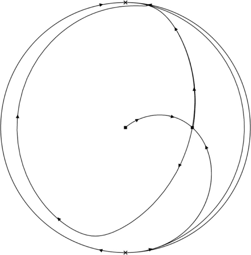
b > 0; c < 0.
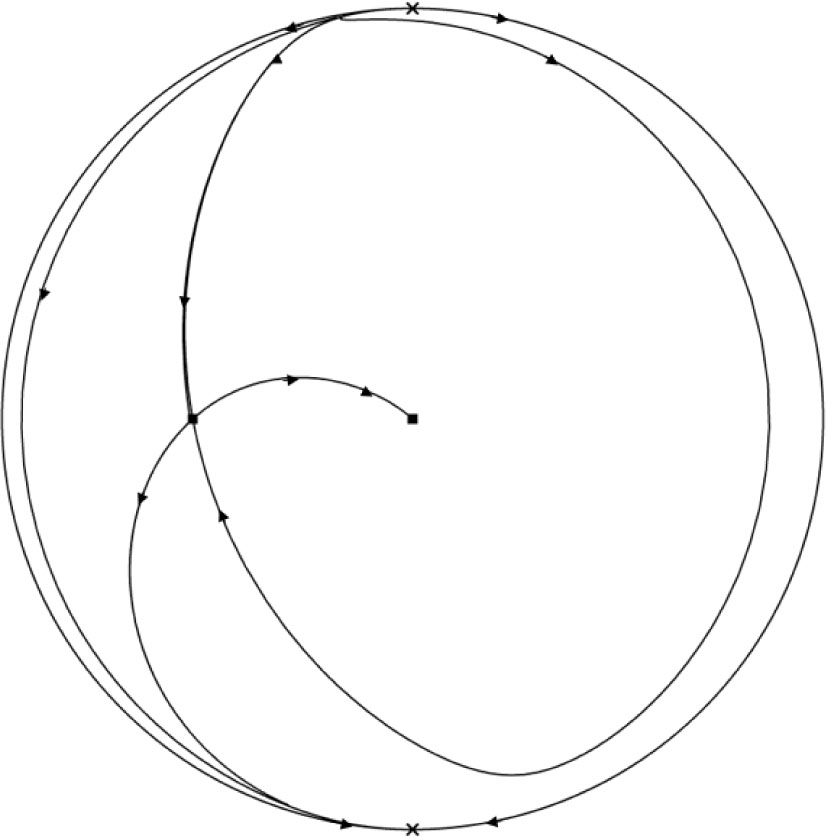
b < 0; c > 0.
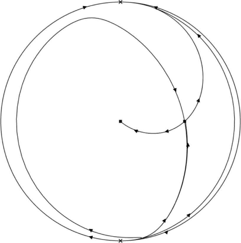
b < 0; c < 0.
7 Final Remarks
In this paper we studied from algebraic point of view and singular points study the five parametric family of linear differential systems that came from the corrigendum of Exercise 11 in [18, § 1.3.3], which we called Polyanin-Zaitsev vector field. We solved the corrected exercise through a series of transformations using Hamiltonian changes of variables. A analysis was also developed to find critical points and their behavior.
References
[1] Guckenheimer J., Nonlinear Oscillations, Dynamical Systems and Bifurcations of Vector Fields, Springer-Verlag New York, 1983.10.1007/978-1-4612-1140-2Suche in Google Scholar
[2] Guckenheimer J., Hoffman K., Weckesser W., The forced Van der Pol equation I: The slow flow and its bifurcations, SIAM J. Applied Dynamical Systems, 2003, 2, 1–35.10.1137/S1111111102404738Suche in Google Scholar
[3] Kapitaniak T., Chaos for Engineers: Theory, Applications and Control, Springer, Berlin, Germany, 1998.10.1007/978-3-642-97719-0Suche in Google Scholar
[4] Nagumo J., Arimoto S., Yoshizawa S., An active pulse transmission line simulating nerve axon, Proc. IRE, 1962, 50, 2061–2070.10.1109/JRPROC.1962.288235Suche in Google Scholar
[5] Nemytskii V.V., Stepanov V.V., Qualitative Theory of Differential Equations, Princeton University Press, Princeton, 1960.10.1515/9781400875955Suche in Google Scholar
[6] Perko L., Differential equations and Dynamical systems, Third Edition, Springer-Verlag New York, Inc, 2001.10.1007/978-1-4613-0003-8Suche in Google Scholar
[7] Van der Pol B., Van der Mark J., Frequency demultiplication, Nature, 1927, 120, 363–364.10.1038/120363a0Suche in Google Scholar
[8] Acosta-Humánez P.B., La Teoría de Morales-Ramis y el Algoritmo de Kovacic, Lecturas Matemáticas, Volumen Especial, 2006, 21–56.Suche in Google Scholar
[9] Acosta-Humánez P.B., Pantazi Ch., Darboux Integrals for Schrodinger Planar Vector Fields via Darboux Transformations, SIGMA Symmetry Integrability Geom. Methods Appl., 2012, 8, 043, https://arxiv.org/abs/1111.0120 arXiv:1111.0120.10.3842/SIGMA.2012.043Suche in Google Scholar
[10] Acosta-Humánez P.B., Perez J., Teoría de Galois diferencial: una aproximación, Matemáticas: Enseãnza Universitaria, 2007, 91–102.Suche in Google Scholar
[11] Acosta-Humánez P.B., Perez J., Una introducción teoría de Galois diferencial, Boletín de Matemáticas Nueva Serie, 2004, 11, 138–149.Suche in Google Scholar
[12] Morales-Ruiz J., Differential Galois Theory and Non-Integrability of Hamiltonian Systems, Birkhäuser, Basel, 1999.10.1007/978-3-0348-0723-4Suche in Google Scholar
[13] Van der Put M., Singer M., Galois Theory in Linear Differential Equations, Springer-Verlag New York, 2003.10.1007/978-3-642-55750-7Suche in Google Scholar
[14] Weil J.A., Constant et polynómes de Darboux en algèbre différentielle: applications aux systèmes différentiels linéaires, Doctoral thesis, 1995.Suche in Google Scholar
[15] Acosta-Humánez P.B., Galoisian Approach to Supersymmetric Quantum Mechanics, PhD Thesis, Barcelona, 2009, https://arxiv.org/abs/0906.3532 arXiv:0906.3532.Suche in Google Scholar
[16] Acosta-Humánez P.B., Blázquez-Sanz D., Non-integrability of some Hamiltonians with rational potentials, Discrete Contin. Dyn. Syst. Ser. B, 2008, 10, 265–293.10.3934/dcdsb.2008.10.265Suche in Google Scholar
[17] Acosta-Humánez P., Morales-Ruiz J., Weil J.-A., Galoisian approach to integrability of Schrödinger Equation, Rep. Math. Phys., 2011, 67(3), 305–374.10.1016/S0034-4877(11)60019-0Suche in Google Scholar
[18] Polyanin A.D., Zaitsev V.F., Handbook of exact solutions for ordinary differential equations, Second Edition, Chapman and Hall, Boca Raton, 2003.10.1201/9781420035339Suche in Google Scholar
[19] Acosta-Humánez P.B., Lázaro J.T., Morales-Ruiz J.J., Pantazi Ch., On the integrability of polynomial fields in the plane by means of Picard-Vessiot theory, Discrete Contin. Dyn. Syst., 2015, 35(5), 1767–1800.10.3934/dcds.2015.35.1767Suche in Google Scholar
[20] Drumortier F., Llibre J., Artés J.C., Qualitative theory of planar differential systems, Springer-Verlag Berlin Heidelberg, 2006.Suche in Google Scholar
© 2019 Rodríguez-Contreras et al., published by De Gruyter
This work is licensed under the Creative Commons Attribution 4.0 Public License.
Artikel in diesem Heft
- Regular Articles
- On the Gevrey ultradifferentiability of weak solutions of an abstract evolution equation with a scalar type spectral operator of orders less than one
- Centralizers of automorphisms permuting free generators
- Extreme points and support points of conformal mappings
- Arithmetical properties of double Möbius-Bernoulli numbers
- The product of quasi-ideal refined generalised quasi-adequate transversals
- Characterizations of the Solution Sets of Generalized Convex Fuzzy Optimization Problem
- Augmented, free and tensor generalized digroups
- Time-dependent attractor of wave equations with nonlinear damping and linear memory
- A new smoothing method for solving nonlinear complementarity problems
- Almost periodic solution of a discrete competitive system with delays and feedback controls
- On a problem of Hasse and Ramachandra
- Hopf bifurcation and stability in a Beddington-DeAngelis predator-prey model with stage structure for predator and time delay incorporating prey refuge
- A note on the formulas for the Drazin inverse of the sum of two matrices
- Completeness theorem for probability models with finitely many valued measure
- Periodic solution for ϕ-Laplacian neutral differential equation
- Asymptotic orbital shadowing property for diffeomorphisms
- Modular equations of a continued fraction of order six
- Solutions with concentration and cavitation to the Riemann problem for the isentropic relativistic Euler system for the extended Chaplygin gas
- Stability Problems and Analytical Integration for the Clebsch’s System
- Topological Indices of Para-line Graphs of V-Phenylenic Nanostructures
- On split Lie color triple systems
- Triangular Surface Patch Based on Bivariate Meyer-König-Zeller Operator
- Generators for maximal subgroups of Conway group Co1
- Positivity preserving operator splitting nonstandard finite difference methods for SEIR reaction diffusion model
- Characterizations of Convex spaces and Anti-matroids via Derived Operators
- On Partitions and Arf Semigroups
- Arithmetic properties for Andrews’ (48,6)- and (48,18)-singular overpartitions
- A concise proof to the spectral and nuclear norm bounds through tensor partitions
- A categorical approach to abstract convex spaces and interval spaces
- Dynamics of two-species delayed competitive stage-structured model described by differential-difference equations
- Parity results for broken 11-diamond partitions
- A new fourth power mean of two-term exponential sums
- The new operations on complete ideals
- Soft covering based rough graphs and corresponding decision making
- Complete convergence for arrays of ratios of order statistics
- Sufficient and necessary conditions of convergence for ρ͠ mixing random variables
- Attractors of dynamical systems in locally compact spaces
- Random attractors for stochastic retarded strongly damped wave equations with additive noise on bounded domains
- Statistical approximation properties of λ-Bernstein operators based on q-integers
- An investigation of fractional Bagley-Torvik equation
- Pentavalent arc-transitive Cayley graphs on Frobenius groups with soluble vertex stabilizer
- On the hybrid power mean of two kind different trigonometric sums
- Embedding of Supplementary Results in Strong EMT Valuations and Strength
- On Diophantine approximation by unlike powers of primes
- A General Version of the Nullstellensatz for Arbitrary Fields
- A new representation of α-openness, α-continuity, α-irresoluteness, and α-compactness in L-fuzzy pretopological spaces
- Random Polygons and Estimations of π
- The optimal pebbling of spindle graphs
- MBJ-neutrosophic ideals of BCK/BCI-algebras
- A note on the structure of a finite group G having a subgroup H maximal in 〈H, Hg〉
- A fuzzy multi-objective linear programming with interval-typed triangular fuzzy numbers
- Variational-like inequalities for n-dimensional fuzzy-vector-valued functions and fuzzy optimization
- Stability property of the prey free equilibrium point
- Rayleigh-Ritz Majorization Error Bounds for the Linear Response Eigenvalue Problem
- Hyper-Wiener indices of polyphenyl chains and polyphenyl spiders
- Razumikhin-type theorem on time-changed stochastic functional differential equations with Markovian switching
- Fixed Points of Meromorphic Functions and Their Higher Order Differences and Shifts
- Properties and Inference for a New Class of Generalized Rayleigh Distributions with an Application
- Nonfragile observer-based guaranteed cost finite-time control of discrete-time positive impulsive switched systems
- Empirical likelihood confidence regions of the parameters in a partially single-index varying-coefficient model
- Algebraic loop structures on algebra comultiplications
- Two weight estimates for a class of (p, q) type sublinear operators and their commutators
- Dynamic of a nonautonomous two-species impulsive competitive system with infinite delays
- 2-closures of primitive permutation groups of holomorph type
- Monotonicity properties and inequalities related to generalized Grötzsch ring functions
- Variation inequalities related to Schrödinger operators on weighted Morrey spaces
- Research on cooperation strategy between government and green supply chain based on differential game
- Extinction of a two species competitive stage-structured system with the effect of toxic substance and harvesting
- *-Ricci soliton on (κ, μ)′-almost Kenmotsu manifolds
- Some improved bounds on two energy-like invariants of some derived graphs
- Pricing under dynamic risk measures
- Finite groups with star-free noncyclic graphs
- A degree approach to relationship among fuzzy convex structures, fuzzy closure systems and fuzzy Alexandrov topologies
- S-shaped connected component of radial positive solutions for a prescribed mean curvature problem in an annular domain
- On Diophantine equations involving Lucas sequences
- A new way to represent functions as series
- Stability and Hopf bifurcation periodic orbits in delay coupled Lotka-Volterra ring system
- Some remarks on a pair of seemingly unrelated regression models
- Lyapunov stable homoclinic classes for smooth vector fields
- Stabilizers in EQ-algebras
- The properties of solutions for several types of Painlevé equations concerning fixed-points, zeros and poles
- Spectrum perturbations of compact operators in a Banach space
- The non-commuting graph of a non-central hypergroup
- Lie symmetry analysis and conservation law for the equation arising from higher order Broer-Kaup equation
- Positive solutions of the discrete Dirichlet problem involving the mean curvature operator
- Dislocated quasi cone b-metric space over Banach algebra and contraction principles with application to functional equations
- On the Gevrey ultradifferentiability of weak solutions of an abstract evolution equation with a scalar type spectral operator on the open semi-axis
- Differential polynomials of L-functions with truncated shared values
- Exclusion sets in the S-type eigenvalue localization sets for tensors
- Continuous linear operators on Orlicz-Bochner spaces
- Non-trivial solutions for Schrödinger-Poisson systems involving critical nonlocal term and potential vanishing at infinity
- Characterizations of Benson proper efficiency of set-valued optimization in real linear spaces
- A quantitative obstruction to collapsing surfaces
- Dynamic behaviors of a Lotka-Volterra type predator-prey system with Allee effect on the predator species and density dependent birth rate on the prey species
- Coexistence for a kind of stochastic three-species competitive models
- Algebraic and qualitative remarks about the family yy′ = (αxm+k–1 + βxm–k–1)y + γx2m–2k–1
- On the two-term exponential sums and character sums of polynomials
- F-biharmonic maps into general Riemannian manifolds
- Embeddings of harmonic mixed norm spaces on smoothly bounded domains in ℝn
- Asymptotic behavior for non-autonomous stochastic plate equation on unbounded domains
- Power graphs and exchange property for resolving sets
- On nearly Hurewicz spaces
- Least eigenvalue of the connected graphs whose complements are cacti
- Determinants of two kinds of matrices whose elements involve sine functions
- A characterization of translational hulls of a strongly right type B semigroup
- Common fixed point results for two families of multivalued A–dominated contractive mappings on closed ball with applications
- Lp estimates for maximal functions along surfaces of revolution on product spaces
- Path-induced closure operators on graphs for defining digital Jordan surfaces
- Irreducible modules with highest weight vectors over modular Witt and special Lie superalgebras
- Existence of periodic solutions with prescribed minimal period of a 2nth-order discrete system
- Injective hulls of many-sorted ordered algebras
- Random uniform exponential attractor for stochastic non-autonomous reaction-diffusion equation with multiplicative noise in ℝ3
- Global properties of virus dynamics with B-cell impairment
- The monotonicity of ratios involving arc tangent function with applications
- A family of Cantorvals
- An asymptotic property of branching-type overloaded polling networks
- Almost periodic solutions of a commensalism system with Michaelis-Menten type harvesting on time scales
- Explicit order 3/2 Runge-Kutta method for numerical solutions of stochastic differential equations by using Itô-Taylor expansion
- L-fuzzy ideals and L-fuzzy subalgebras of Novikov algebras
- L-topological-convex spaces generated by L-convex bases
- An optimal fourth-order family of modified Cauchy methods for finding solutions of nonlinear equations and their dynamical behavior
- New error bounds for linear complementarity problems of Σ-SDD matrices and SB-matrices
- Hankel determinant of order three for familiar subsets of analytic functions related with sine function
- On some automorphic properties of Galois traces of class invariants from generalized Weber functions of level 5
- Results on existence for generalized nD Navier-Stokes equations
- Regular Banach space net and abstract-valued Orlicz space of range-varying type
- Some properties of pre-quasi operator ideal of type generalized Cesáro sequence space defined by weighted means
- On a new convergence in topological spaces
- On a fixed point theorem with application to functional equations
- Coupled system of a fractional order differential equations with weighted initial conditions
- Rough quotient in topological rough sets
- Split Hausdorff internal topologies on posets
- A preconditioned AOR iterative scheme for systems of linear equations with L-matrics
- New handy and accurate approximation for the Gaussian integrals with applications to science and engineering
- Special Issue on Graph Theory (GWGT 2019)
- The general position problem and strong resolving graphs
- Connected domination game played on Cartesian products
- On minimum algebraic connectivity of graphs whose complements are bicyclic
- A novel method to construct NSSD molecular graphs