Determination of soil–water characteristic curves by using a polymer tensiometer

Martin Wijaya; Aswin Lim; Paulus Pramono Rahardjo; Alfrendo Satyanaga; Abdul Halim Hamdany; Glenn Adriel Adiguna

doi:10.1515/jmbm-2024-0007

Article Open Access

Determination of soil–water characteristic curves by using a polymer tensiometer

Martin Wijaya , Aswin Lim , Paulus Pramono Rahardjo , Alfrendo Satyanaga , Abdul Halim Hamdany and Glenn Adriel Adiguna

Published/Copyright: August 1, 2024

Published by

Become an author with De Gruyter Brill

Submit Manuscript Author Information

From the journal Journal of the Mechanical Behavior of Materials Volume 33 Issue 1

Abstract

Recently, rainfall-induced slope failure has struck Cimanggung village, West Java province, Indonesia. In order to anticipate future slope failures due to rainfall, an unsaturated slope stability analysis is compulsory. Precise information on the soil–water characteristic curve (SWCC) is required to conduct an accurate unsaturated soil analysis. In this article, a procedure to obtain SWCC by using a polymer tensiometer for Cimanggung village is proposed. Considering the long period of time needed to obtain the measured data, some prediction methods are available. The measured SWCCs are then compared with SWCCs based on two prediction methods. Chin’s 1-point and Perera et al.’s methods are applied as the prediction methods and then compared with the measured SWCCs. It could be concluded that Chin’s 1-point method yields a close estimation within the suction range. Meanwhile, the Perera et al. method underestimates the air entry value, and the predicted curve deviates significantly with the measured SWCC. Hence, Chin’s 1-point method is recommended for predicting SWCCs in Cimanggung Village.

Keywords: polymer tensiometer; unsaturated soil; suction measurement; SWCC; Cimanggung

1 Introduction

The role of the soil–water characteristic curve (SWCC) is not limited to serving as an input parameter for the transient flow analysis in unsaturated soil [1] but is also one of the most reliable parameters to estimate the shear strength [2–8] and permeability [9–13] of unsaturated soil which are a function of soil suction. Zhai et al. [14] used a contact angle method to estimate SWCC from the grain-size distribution of coarse-grained soil. Zhai et al. [15,16] used both “ink-bottle” and “rain-drop” effects to estimate the hysteresis of SWCC and unsaturated permeability of soil. The hysteresis path of SWCC and unsaturated permeability of soil resulting from wetting–drying cycles is important to conduct slope stability analysis [17].

There are three types of SWCCs [18], which are the gravimetric-based SWCC (SWCC-w), the volumetric-based SWCC (SWCC-θ), and the degree of saturation-based SWCC (SWCC-S). SWCC-w is the easiest to obtain as it is not required to measure the volume change of unsaturated soil specimens due to the change in soil suction [19–21]. The effect of density and stress dependency on SWCC-w has also been investigated by several researchers [22–26]. The investigations have shown that the effect of density (either due to compaction or consolidation) on coarse-grained and fine-grained soils only affects the initial part of the curve and will merge into the virgin drying line, as illustrated in Figure 1. However, it is important to note that the input for the flow analysis in unsaturated soil requires SWCC-θ, while the determination of the unsaturated permeability function and air entry value (AEV) requires SWCC-S [11,12,18]. Hence, it is imperative to obtain all the three SWCCs. For coarse-grained soil, there will be no change in volume due to the change in soil suction. Hence, SWCC-w, SWCC-θ, and SWCC-S will provide similar information [18]. However, there will be a significant change in soil volume due to the change in soil suction when it comes to fine-grained soil. Suction on fine-grained soil can be extremely high, especially when there is a vegetation on the sloping ground. The significant increase in soil suction may affect the hydraulic properties of unsaturated soil [27]. Hence, conversion between SWCCs will be very important. As it is difficult to measure the volume change during the SWCC test, it is recommended to construct a shrinkage curve (a curve that represents a change in the void ratio due to the change in the gravimetric water content) to convert SWCC-w to SWCC-θ and SWCC-S [18,28,29].

Figure 1

Effect of density on SWCC-w [24].

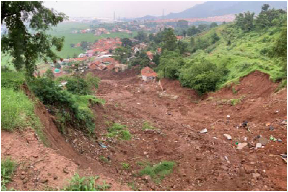
On 9 January 2021, heavy rainfall (143 mm/day) induced slope failure at Cimanggung (Figure 2) and caused significant death toll and destruction of properties in the landslide vicinity [30]. Due to the landslide, most of the people living in the landslide vicinity were temporarily evacuated and arose a necessity to take a decision on whether the housing in the landslide area could be reconstructed after the landslide. Rainfall-induced slope failure has been assessed in the Cimanggung slope using estimated unsaturated soil properties [31]. In order to make a proper assessment of the potential of a future landslide due to the rainfall that might occur, it is important to obtain an SWCC, which is one of the main soil properties in unsaturated soil analysis [18]. In this article, an SWCC for volcanic soil in Indonesia is proposed which can be applied as a volcanic soil SWCC database for other regions in the world. SWCC can be obtained from direct measurement of suction using a tensiometer. However, conventional tensiometers generally only be able to measure suction up to 90 kPa. In this article, the focus is on developing a procedure to determine SWCC-w from the debris of the slope and how it is compared with a typical prediction method which is used as no data are available. The objective of this article is to establish a procedure to obtain SWCC-w, SWCC-θ, and SWCC-S in the most economical way by using a polymer tensiometer developed by Umwelt-Geräte-Technik (UGT) that can measure the matric suction up to 1,500 kPa, and there is no requirement for maintenance (flushing due to diffusion), so that it is possible to do a long-term measurement. Comparison will also be carried out to evaluate the suitability of some prediction methods for soil at Cimanggung village.

Figure 2

Aerial photo of Cimanggung slope failure.

2 Background theory

SWCC-θ could be determined once a shrinkage curve is obtained as follows:

(1) θ ( s ) = w ⋅ G s 1 + e ,

where θ(s) is the volumetric water content as a function of soil suction and w is the gravimetric water content that can be obtained from SWCC-w and is a function of soil suction and void ratio (e). Those parameters could be obtained from the shrinkage curve. Similarly, SWCC-S can also be obtained through the following relationship:

(2) S r ( s ) = w ⋅ G s e .

SWCC can be constructed by either reducing the water content of the soil and then measuring its suction or by controlling the soil suction and then measuring the water content. Suction measurement can be done either by using a direct measurement method where the pore water pressure (u _w) is directly measured to determine the soil suction or an indirect measurement method in which other properties are used to determine soil suction [32]. Regardless of the methods that are used to construct the SWCC, the range of suction that can be measured is limited by the apparatus. For instance, a tensiometer (direct measurement) is unable to measure the pore pressure less than −101 kPa due to the cavitation phenomenon [33–35]. A way to overcome the limitation of direct measurement is either by using an axis translation apparatus [34,36] or by employing a high-capacity tensiometer (HCT) [32,33,37–42].

In the axis translation apparatus, the air pressure (u _a) is increased such that the pore water pressure (u _w) is also increased to avoid cavitation [34,36]. The maximum air pressure that can be applied depends on the amount of air that enters the high-air entry (HAE) disk, with the maximum value typically around 1,500 kPa. The equilibrium time required to measure the soil suction may range from a few hours to days depending on the type of soil. An HCT is developed to directly measure soil suction as high as 1,500 kPa. The reason behind HCT can extend the range of suction measurement beyond 101 kPa is that due to the use of demineralized water, the water in the small water compartment between the transducer and the HAE disk is pressurized under very high pressure to remove all the air bubbles in the water compartment [37,38]. The problem with HCT is that once it is used for a long period of time, it may cavitate despite not reaching its maximum capacity, and once it is cavitated, the HCT needs to be repressurized [41].

In the indirect measurement method, the soil suction is measured by using other properties such as filter paper [43,44] or chilled mirror hygrometer [45]. The indirect measurement typically has a much wider range of suction measurements but unsuitable for the low suction range [46]. Looking at the limitations that come from different apparatuses, it is difficult to obtain the entire range of SWCCs [47]. While it is possible to use different apparatuses to obtain the entire range of SWCCs, the cost of purchasing different apparatuses to measure soil suction makes it practically difficult for industrial laboratories to use it as a routine practice. Another problem is the test duration to obtain sufficient data to construct SWCCs.

The most recent development in suction measurement is using a polymer-based or an osmotic tensiometer [47–53]. In a polymer-based tensiometer, a polymer solution is placed inside a membrane that is permeable to the soil solution but impermeable to the polymer solution [50]. The polymer tensiometer is pre-saturated so that the polymer solution absorbs the water and generates a swelling pressure, sometimes referred to as the osmotic pressure [47]. The maximum osmotic pressure which is obtained through pre-saturation is referred to as P _ref. When the polymer tensiometer is in contact with unsaturated soil, there will be a pressure drop inside the polymer tensiometer (P _current). The drop in pressure is assumed to be equal to the increase in uncorrected soil suction (s _uncor), and hence soil suction can be calculated as follows [47,50]:

(3) s uncor = p ref − p current .

The first polymer tensiometer was perhaps developed by Peck and Rabbidge [51]. The conventional tensiometer generally can only measure suction up to 90 kPa. The polymer tensiometer is attractive due to its potential to measure high suction, with the maximum suction measured to be about 1,000–1,500 kPa; it can be pre-saturated using a simple water bath without any water pressure to reach its full capacity, has no issue with cavitation, and hence can be easily adopted for in situ measurement [47–50,53]. However, several issues related to polymer tensiometer have been addressed by Bocking and Fredlund [54], such as the polymer tensiometer suffering gradual loss of pressure (pressure decay), unknown zero drift, temperature effects, and slow equilibration times, which then halted the development of polymer tensiometer at that time [50].

Figure 3a shows the decay in osmotic pressure measured by van der Ploeg [50], while Figure 3b shows the effect of temperature on the osmotic pressure. Figure 4 shows the decay in suction and the effect of temperature on the suction measurement using a polymer tensiometer conducted by Hamdany et al. [47]. Pressure decay is suspected due to polymer degradation or by diffusion of some smaller-sized polymer molecules through the membrane [47,50] and hence requires a correction to be applied. van der Ploeg [50] observed that the pressure decay gradually became less (or exponential decay) and proposed the following correction for pressure decay:

(4) π t = b exp − ( t / τ ) c ,

where π _t is the pressure decay correction, t is the time, and b, τ, and c are curve-fitting parameters. On the other hand, Peck and Rabbidge [52] and Hamdany et al. [47] observed a linear decay. Hamdany et al. [47] proposed a linear correction as follows:

(5) π t = m d ( t − t 0 ) ,

where m _d is the curve-fitting parameter and t ₀ is the time when the probe is fully saturated. For temperature correction, van der Ploeg [50] proposed a quadratic function as follows:

(6) P T − P 0 P 0 = C 1 T − T 0 T 0 2 + C 2 T − T 0 T 0 + C 3 ,

where P _t is the pressure at temperature T, P ₀ is the reference pressure at reference temperature T ₀, and C ₁, C ₂, and C ₃ are curve-fitting parameters. An example of the fitted equation is shown in Figure 3b. Hamdany et al. [47] proposed employing linear regression to fit the change in suction (Ds _t) with temperature, as shown in Figure 4b. Soil suction (uncorrected with pressure decay) can then be calculated as follows:

(7) s t = s uncor − Δ s T .

Figure 3

(a) Pressure decay and (b) temperature effect [50].

Figure 4

(a) Effect of pressure decay and temperature effect on suction measurement and (b) temperature correction [47].

The corrected soil suction (s) can then be corrected as follows [47]:

(8) s = s t − Δ s d .

Figure 5 shows the correction for temperature and pressure conducted by Hamdany et al. [47]. Extensive research has been carried out by Degré et al. [48] to compare the SWCC obtained from the polymer tensiometer and the matric potential sensor (MPS) with a reference SWCC (constructed by using five intact soil cores), and by van der Ploeg et al. [53] where a sand box (0–9.8 kPa suction), suction plates (9.8–59 kPa suction), and a pressure plate (100–1,500 kPa suction) are used to construct the SWCC (Figure 6). It is shown that the polymer tensiometer appears to agree very well with the reference curve, which shows the capability of the polymer tensiometer. It is interesting to note that there appears to be no decay in the polymer tensiometer used by Degré et al. and van der Ploeg et al. [48].

Figure 5

Correction for temperature and pressure [47].

Figure 6

Comparison between MPS and the polymer tensiometer (POT) with a reference water retention curve from van der Ploeg et al. [53] conducted by (Degré et al. [48].

UGT developed a polymer tensiometer (Figure 7), which is referred to as a full-range tensiometer (FRT). The polymer-based tensiometer is typically affected with the decay issue, as described in the literature review. However, the UGT polymer tensiometer is unaffected by decay. The capacity of the UGT polymer tensiometer is around 2,000 kPa. The UGT polymer tensiometer is claimed to be maintenance-free and can remain in the field for a very long period due to low power consumption. The UGT polymer tensiometer measurement is also reliable in difficult media such as in saline sites. The temperature correction to the P _ref is given by:

(9) p ref = C T 1 ⋅ T current 2 + C T 2 ⋅ T current + P 0 ,

where C _T1 and C _T2 are curve-fitting parameters, P ₀ is the reference pressure at 0°C, and T _current is the current temperature. Decay correction is only required when there is an offset in the P ₀. While the UGT polymer tensiometer is actually meant for in situ measurement, it is of interest to use the UGT polymer tensiometer to obtain SWCC in the lab which makes the tensiometer attractive as it can be used in the lab and on the site.

Figure 7

Components of FRT.

As obtaining SWCCs takes a very long time to finish, the use of an estimation method is sometimes preferred to obtain the SWCC, especially for the case where a quick decision has to be made. Perera et al. [55] proposed the use of Fredlund and Xing’ [56] degree of saturation-based SWCC (SWCC-S), which is expressed as follows:

(10) S r ( s ) = C ( s ) ln exp ( 1 ) + s a f n f m f C ( s ) = 1 − ln 1 + s ψ r ln 1 + 10 6 ψ r .

Determination of a _f, n _f, m _f, and ψ _r depends on the plasticity index (PI) and percent passing sieve No. 200 (P ₂₀₀). Soil is considered as non-plastic granular soil if PI.P ₂₀₀/100 < 1, while it is considered as plastic soil when PI.P ₂₀₀/100 > 1. For non-plastic granular soil, Fredlund and Xing’s [56] empirical parameters are given as follows:

(11a) a f = max ( 1.14 a − 0.5 , 1 ) a = − 2.79 − 14.1 log ( D 20 ) − 1.9 × 10 − 6 P 200 4.34 + 7 log ( D 30 ) + 0.055 D 100 ,

(11b) D 100 = 10 40 m 1 p + log ( D 60 ) ,

(11c) m 1 p = 30 [ log ( D 90 ) − log ( D 60 ) ] ,

(11d) n f = 0.936 b − 3.8 ,

(11e) b = 5.39 − 0.29 ln P 200 D 90 D 10 + 3 D 0 0.57 + 0.021 P 200 1.19 m 1 0.1 ,

(11f) D 0 = 10 − 30 m 2 p + log ( D 30 ) ,

(11g) m 2 p = 20 [ log ( D 30 ) − log ( D 10 ) ] ,

(11h) m f = 0.26 exp ( 0.758 c ) + 1.4 D 10 ,

(11i) c = log ( m 2 p 1.15 ) − 1 − 1 n f ,

(11j) ψ r = 100 ,

where D _x is the particle size at percent passing x. For plastic soil, Fredlund and Xing’s [56] empirical parameters are given as follows:

(11k) a f = 32.853 ln P 200 100 PI + 32.438 ,

(11l) n f = 1.421 P 200 100 PI − 0.3185 ,

(11m) m f = − 0.2154 ln P 200 100 PI + 0.7145 ,

(11n) ψ r = 500 .

Another method is to use Chin’s 1-point method [57]. According to Chin’s 1-point method, one pair of suction and volumetric water content data is required. The advantage of this method is that as measuring a single suction and water content can be done relatively quick (either in the laboratory or at the site), prediction can be done reasonably fast with a higher degree of confidence (1 data definitely correct). The Chin 1-point method adopted Fredlund and Xing’s [56] volumetric water content-based SWCC (SWCC-θ), where the empirical parameters in Fredlund and Xing [56] are correlated with a single empirical parameter χ. In Chin’s 1-point method, the soil is classified either as fine-grained soil (P ₂₀₀ > 30%) or as coarse-grained soil (P ₂₀₀ < 30%). For fine-grained soil, Fredlund and Xing’s [56] empirical parameters are given as follows:

(12a) a f = − 2.4 χ + 722 ,

(12b) n f = 0.07 χ 0.4 ,

(12c) m f = 0.015 χ 0.7 ,

(12d) ψ r = 914 exp [ − 0.002 ( χ ) ] .

While for coarse-grained soil, Fredlund and Xing’s [56] empirical parameters are given as follows:

(12e) a f = 0.53 ( D 50 ) − 0.96 ,

(12f) n f = χ ,

(12g) m f = − 0.23 ln ( χ ) + 1.13 ,

(12h) ψ r = 100 .

Chin et al. [57] recommended that the parameter χ is determined by using soil suction between 300 and 500 kPa. However, predictive methods rely on the soil data which are used as a database. Hence, evaluating predictive methods with actual measurement is important to increase confidence in using a predictive method in practice.

3 Materials and methods

The procedure to obtain SWCC-w, SWCC-θ, and SWCC-S by using the UGT polymer tensiometer follows the flow chart shown in Figure 8. As it is difficult to obtain undisturbed soil samples of sufficient size, it is recommended to obtain disturbed soil samples which are then reconstituted to obtain SWCC-w by using the polymer tensiometer. Undisturbed soil samples are important to characterize the soil state at the site, which could be applied to correct the SWCC-w in the field condition and to estimate the shrinkage curve.

Figure 8

Proposed procedure to obtain SWCC-θ and SWCC-S.

Pre-saturation and calibration of the UGT polymer tensiometer are conducted by submerging the tensiometer in a water chamber until the pressure reading reaches its maximum value. Natural fluctuation of temperature and pressure is recorded as shown in Figure 9. No apparent decay is observed during the calibration process. In this research, the quadratic function as described in Eq. (9) is used to calibrate the polymer tensiometer with temperature. C _T1, C _T2, and P ₀ values obtained from the calibration result are −0.0765, 21.871, and 1523.41, respectively.

Figure 9

Calibration of FRT.

Soil samples are obtained from the landslide area at Cimanggung village, West Jaya Province, Indonesia (Figure 10). The undisturbed soil sample is obtained from the site to determine the natural state of soil properties. The soil properties are shown in Table 1.

Figure 10

Soil materials located at the landslide area.

Table 1

Basic soil properties

Soil properties	Values
Specific gravity, G _s	2.53
Liquid limit, LL	54
Plastic limit, PL	31
Index plasticity, IP	23
Bulk density, γ _b (kN/m³)	17.7
Dry density, γ _d (kN/m³)	12.6
Natural water content, w _n (%)	36.47
Void ratio, e	1.0
Porosity, n	0.5
Grain size distribution (USCS)
Sand (%)	15.83
Silt (%)	43.6
Clay (%)	40.6

Due to the size of the UGT polymer tensiometer, a larger sample diameter is required. Another batch of disturbed soil samples is obtained in order to be reconstituted and then compacted. The initial water content of the compacted soil is about 32.3%. An SWCC is then constructed by air-drying the soil specimen, and the soil suction is measured using the polymer tensiometer shown in Figure 11. The weight of soil is also recorded in order to determine the gravimetric water content (w) of the soil. Once the soil suction reaches around 2,000 kPa, the test is deemed completed. The van Genuchten [10] (VG) SWCC equation was used to curve fit the data points from the polymer tensiometer, which is given as follows

(13) w ( s ) = w r + ( w s − w r ) [ 1 + a v s ) n v ] m v ,

where w _s is the saturated gravimetric water content; w _r is the residual gravimetric water content; and a _v, n _v, and m _v are VG’s curve-fitting parameters.

Figure 11

Installation of FRT.

As it is of interest to obtain SWCC of the soil at in situ conditions, it is of interest to correct gravimetric-based SWCC (SWCC-w) according to the density of the undisturbed soil sample. Correction for SWCC-w under different densities can be done by using Wijaya and Leong [24], which is illustrated in Figure 1 where the effect of density can be reflected by the change in the saturated gravimetric water content (w _s,0 to w _s,f) and change in the matric suction at the intersection between the initial drying line and the virgin drying line (from s _2,0 to s _2,f). Wijaya and Leong [58] proposed an SWCC equation that uses physically significant parameters and is given as follows:

(14a) w ( s ) = w s − m 1 log s s 1 − T 2 ( log s , log s 1 , log s 2 , m 2 , m 1 , k 2 ) − T 3 ( log s , log s 1 , log s 3 , m 3 , m 2 , k 3 ) ,

(14b) T i ( x , x 1 , x i , m i , m i − 1 , k i ) = 1 2 ( m i − m i − 1 ) ( x − x 1 ) + 1 k i ln cosh [ k i ( x − x i ) ] cosh [ k i ( x i − x 1 ) ] ,

where m _i is the slope of the linear segment i, s _i is the matric suction at the intersection between segment i and segment i − 1, k _i is the curvature parameter between segment i and segment i − 1, m ₁ is the slope of the initial drying line, s₁ is the matric suction at w _s, and n is the number of linear segments where for unimodal SWCC, n = 3. Hence, by changing w _s in Eq. (14a) into w _s,f and s ₂ into s _2,f, correction for the density can be done. The value of s _2,f can be obtained as follows [24]:

(15) s 2 , f = s 2 , 0 10 ( w s,0 − w s,f ) / ( m 2 − m 1 ) .

Conversion between SWCC-w and volumetric-based SWCC (SWCC-θ) and degree of saturation-based SWCC (SWCC-S) can be done by using the shrinkage curve [12,28] by using Eqs. (1) and (2). Leong and Wijaya [29] proposed a shrinkage curve equation for normal shrinkage as follows:

(16) e ( w ) = e min + G s 2 S w + 1 c ln cosh ( c ( w − SL ) ) cosh ( c ⋅ SL ) ,

where e _min is the minimum void ratio, SL is the shrinkage limit, and c is the shrinkage curve empirical parameter, which can be obtained as follows [59]:

(17) c = 4.32 G s S 0 e min .

SL was estimated by using LL and PL based on the Casagrande method [60,61] where SL can be determined as follows:

(18) SL = 46.355 LL + 43.5 PI + 46.355 − 43.5 .

The minimum void ratio (e _min) can be estimated through the following relationship [18,28]:

(19) e min SL = G s S 0 .

4 Test results and discussion

Figure 12 shows the SWCC of the Cimanggung soil fitted with the VG [10] SWCC equation with the curve-fitting parameters for the VG [10] SWCC equation shown in Table 2. It can be seen that the UGT polymer tensiometer measurement results show good fitting with the VG equation. In order to correct the density of the reconstituted soil into the in situ density, parameters for Wijaya and Leong [58] must first be determined to fit the SWCC determined from the VG [10] SWCC equation and then corrected for the in situ density according to the procedure described in the study of Wijaya and Leong [24]. Parameters for the Wijaya and Leong [58] SWCC equation are shown in Table 3, while the corrected curve is shown in Figure 12.

Figure 12

SWCC based on FRT.

Table 2

VG curve-fitting parameters

Curve-fitting parameters	Values
a _v	7.2 × 10⁻⁷
n _v	0.670
m _v	37.712
w _r (%)	0.096
w _s (%)	32.332

Table 3

Physically significant parameters

Reconstituted soil
w	32.33	%
w = 32.33%	m _i	s _i (kPa)	k _i
1	0.18	0.1
2	18.01	570.0	1.15
3	0.0003	32500.0	3.20
In situ density
w	39.53	%
w = 35.67%	m _i	s _i (kPa)	k _i
1	0.18	0.1
2	18.01	224.9	1.15
3	0.0003	32500.0	3.20

According to Eq. (18), SL is 22, and e _min determined from Eq. (19) is 0.548, as shown in Table 4. Hence, by using Eq. (16), the shrinkage curve can be obtained and is shown in Figure 13. The shrinkage curve can then be used to convert SWCC-w, which has been corrected for in situ density, into SWCC-θ and SWCC-S.

Table 4

Parameters of the shrinkage curve

Required parameters	Values
G _s	2.53
S ₀ (%)	100
SL	22
e _min	0.548
C	9

Figure 13

Obtained shrinkage curve.

Figure 14 shows the SWCC-θ obtained from the measurement (corrected with in situ density) and also SWCC-θ estimated based on Chin’s 1-point method. The sensitivity study on Chin’s 1-point method was carried out by using two data points. The first data point was observed at the soil suction of 341 kPa, and the second data point was at the soil suction of 1,111 kPa. Parameters for the Chin’s 1-point method are shown in Table 5. It is important to note that the range of measurements is only up to 2,000 kPa, and it shows that the measured SWCC-θ and SWCC-θ estimated from Chin’s 1-point method (predicted by using 341 kPa suction and 1,111 kPa suction) agree very well in this measurement range. The difference in SWCC beyond the range of measurements could be due to the lack of data points which affects the shape of SWCC.

Figure 14

SWCC-θ obtained from our measurement and the Chin-1 point method.

Table 5

Chin’s 1-point method empirical parameters

Empirical parameters	Values (fit 341 kPa)	Values (fit 1,111 kPa)
χ	67.457	98.183
a _f	560.104	486.361
n _f	0.377	0.438
m _f	0.286	0.372
h _r	798.645	751.044
θ _s	0.501	0.501

Figure 15 shows the measured SWCC-S along with estimated SWCC from the study of Perera et al. [55] and from Chin’s 1-point method. SWCC-θ from Chin’s 1-point method is converted into SWCC-S by using the shrinkage curve. It is shown that Chin’s 1-point method for fit at 341 and 1,111 kPa have roughly the same AEV. However, Perera et al.’s [55] SWCC-S equation underestimated the AEV, and the curve deviated significantly with the measured SWCC. It is understandable that Chin’s 1-point method gives higher accuracy as it is based on 1 data point. However, considering that obtaining 1 data point is not difficult, it is recommended to use Chin’s 1-point method to estimate both SWCC-θ and SWCC-S. Chin’s 1-point method can also be applied by inserting the polymer tensiometer in situ and directly taking the in situ soil for water content measurement. Such procedures allow for rapid and reliable SWCC estimation. The SWCCs can then be used as input parameters along with an unsaturated permeability function to assess the effect of rainfall infiltration on Cimanggung slope failure.

Figure 15

SWCC-S obtained from our measurement and the Perera et al. [55] method.

5 Conclusions

Determination of SWCC on slope failure is difficult due to the uncertainty in determining the density of the debris as the soil has been altered from its original condition (before slope failure). In this article, a new method and procedure to generate SWCC-w, SWCC-θ, and SWCC-S for soil located at slope failure by using the full range of suction has been developed. The key findings are as follows:

In this procedure, it is recommended to obtain the soil sample from the debris, reconstitute the soil sample, and then obtain the SWCC-w.
The validation of the new procedure has been done to obtain the SWCC of reconstituted soil located at the Cimanggung village. SWCC-w, SWCC-θ, and SWCC-S corrected for in situ density have been obtained.
The measured SWCC is also compared with those of Chin’s 1-point method [57] and Perera et al.’s [55] method.

It could be concluded that Chin’s 1-point method yields a close estimation within the suction range. Meanwhile, the Perera et al. method underestimates the AEV and the predicted curve deviates significantly from the measured SWCC. Hence, Chin’s 1-point method is recommended for predicting SWCCs in Cimanggung Village and used as the volcanic soil SWCC database.

Acknowledgement

The authors would like to thank Parahyangan Catholic University for the support, P.T. Geotechnical Engineering Consultant for providing the data, documentation, and visual inspection at the site, and Wykeham Farrance LTD for providing the full-range tensiometer.

Funding information: The authors state no funding was involved.
Author contributions: All authors have accepted responsibility for the entire content of this manuscript and approved its submission.
Conflict of interest: The authors declare no conflict of interest.

References

[1] Fredlund DG, Rahardjo H, Fredlund MD. Unsaturated soil mechanics in Engineering practice. Hoboken, New Jersey: John Wiley & Sons, Inc; 2012.10.1002/9781118280492Search in Google Scholar

[2] Bao C, Gong B, Zhan L, editors. Keynote Lecturer, Properties of unsaturated soils and slope stability of expansive soils. Proceedings of the 2nd International Conference on Unsaturated Soils (UNSAT 98). Beijing, China: International Academic; 1998.Search in Google Scholar

[3] Goh SG, Rahardjo H, Leong EC. Shear strength equations for unsaturated soil under drying and wetting. ASCE J Geotech Geoenviron Eng. 2010;136(4):594–606.10.1061/(ASCE)GT.1943-5606.0000261Search in Google Scholar

[4] Khalili N, Khabbaz MH. A unique relationship for c for the determination of the shear strength of unsaturated soils. Géotechnique. 1998;48(5):681–7.10.1680/geot.1998.48.5.681Search in Google Scholar

[5] Lee IM, Sung SG, Cho GC. Effect of stress state on the unsaturated shear strength of a weathered granite. Can Geotech J. 2005;42(2):624–31.10.1139/t04-091Search in Google Scholar

[6] Rassam DW, Cook FJ. Predicting the shear strength envelope of unsaturated soils. Geotech Test J. 2002;25(2):215–20.10.1520/GTJ11365JSearch in Google Scholar

[7] Rassam D, Williams D. Unsaturated hydraulic conductivity of mine tailings under wetting and drying conditions. Geotech Test J. 1999;22(2):144–52.10.1520/GTJ11273JSearch in Google Scholar

[8] Tekinsoy MA, Kayadelan C, Keskin MS, Soylemaz M. An equation for predicting shear strength envelope with respect to matric suction. Comput Geotech. 2004;31(7):589–93.10.1016/j.compgeo.2004.08.001Search in Google Scholar

[9] Hunt AG. Comparing van Genuchten and Percolation theoretical formulations of the hydraulic properties of unsaturated media. Vadose Zone J. 2004;3(4):1483–8.10.2113/3.4.1483Search in Google Scholar

[10] van Genuchten MT. A closed-form equation for predicting the hydraulic conductivity of unsaturated soils. Soil Sci Soc Am J. 1980;44(5):892–8.10.2136/sssaj1980.03615995004400050002xSearch in Google Scholar

[11] Wijaya M, Leong EC. Discussion of “Permeability function for oil sands tailings undergoing volume change during drying”. Can Geotech J. 2019;56(2):300–2.10.1139/cgj-2018-0136Search in Google Scholar

[12] Zhang F, Wilson GW, Fredlund DG. Permeability function for oil sands tailings undergoing volume change during drying. Can Geotech J. 2017;55(2):191–207.10.1139/cgj-2016-0486Search in Google Scholar

[13] Fredlund DG, Xing A, Huang S. Predicting the permeability function for unsaturated soils using the soil-water characteristic curve. Can Geotech J. 1994;31(4):533–46.10.1139/t94-062Search in Google Scholar

[14] Zhai Q, Rahardjo H, Satyanaga A, Dai G. Estimation of the soil-water characteristic curve from the grain size distribution of coarse-grained soils. Eng Geol. 2020;267:105502.10.1016/j.enggeo.2020.105502Search in Google Scholar

[15] Zhai Q, Rahardjo H, Satyanaga A, Zhu Y, Dai G, Zhao X. Estimation of wetting hydraulic conductivity function for unsaturated sandy soil. Eng Geol. 2021;285:106034.10.1016/j.enggeo.2021.106034Search in Google Scholar

[16] Zhai Q, Rahardjo H, Satyanaga A, Dai G, Du Y. Estimation of the wetting scanning curves for sandy soils. Eng Geol. 2020;272:105635.10.1016/j.enggeo.2020.105635Search in Google Scholar

[17] Ni J, Gu J, Zhao X. A hypoplastic model for unsaturated sand accounting for drying and wetting cycles. Comput Geotech. 2024;165:105879.10.1016/j.compgeo.2023.105879Search in Google Scholar

[18] Wijaya M, Leong EC, Rahardjo H. Effect of shrinkage on air-entry value of soils. Soils Found. 2015;55(1):166–80.10.1016/j.sandf.2014.12.013Search in Google Scholar

[19] Zhai Q, Zhu Y, Rahardjo H, Satyanaga A, Dai G, Gong W, et al. Prediction of the soil–water characteristic curves for the fine-grained soils with different initial void ratios. Acta Geotech. 2023;18(10):5359–68.10.1007/s11440-023-01833-4Search in Google Scholar

[20] Zhai Q, Rahardjo H, Satyanaga A, Dai G-L, Du Y-J. Effect of the uncertainty in soil-water characteristic curve on the estimated shear strength of unsaturated soil. J Zhejiang Univ-Sci A. 2020;21(4):317–30.10.1631/jzus.A1900589Search in Google Scholar

[21] Qian Z, Harianto R, Alfrendo S. Uncertainty in the estimation of hysteresis of soil–water characteristic curve. Environ Geotech. 2019;6(4):204–13.10.1680/jenge.17.00008Search in Google Scholar

[22] Salager S, El Youssoufi MS, Saix C. Definition and experimental determination of a soil-water retention surface. Can Geotech J. 2010;47(6):609–22.10.1139/T09-123Search in Google Scholar

[23] Jotisankasa A, Ridley A, Coop M. Collapse behavior of compacted silty clay in suction-monitored oedometer apparatus. J Geotech Geoenviron Eng. 2007;133(7):867–77.10.1061/(ASCE)1090-0241(2007)133:7(867)Search in Google Scholar

[24] Wijaya M, Leong EC. Modelling the effect of density on the unimodal soil-water characteristic curve. Géotechnique. 2017;67(7):637–45.10.1680/jgeot.15.P.270Search in Google Scholar

[25] Salager S, Ferrari A, Nuth M, Laloui L. Investigations on water retention behaviour of deformable soils. Unsaturated Soils-Alonso & Gens (eds). Barcelona, Spain: Taylor & Francis Group; 2011. p. 485–90.10.1201/b10526-70Search in Google Scholar

[26] Yao Y, Ni J, Li J. Stress-dependent water retention of granite residual soil and its implications for ground settlement. Comput Geotech. 2021;129:103835.10.1016/j.compgeo.2020.103835Search in Google Scholar

[27] Bordoloi S, Ni J, Ng CWW. Soil desiccation cracking and its characterization in vegetated soil: A perspective review. Sci Total Environ. 2020;729:138760.10.1016/j.scitotenv.2020.138760Search in Google Scholar PubMed

[28] Fredlund MD, Wilson GW, Fredlund DG. Representation and estimation of the shrinkage curve. In: Jucá JFT, de Campos TMP, Marinho FAM, editors. 3rd International Conference on Unsaturated Soils (UNSAT 2002). Recife, Brazil; 2002. p. 145–9.Search in Google Scholar

[29] Leong EC, Wijaya M. Universal soil shrinkage curve equation. Geoderma. 2015;237–238:78–87.10.1016/j.geoderma.2014.08.012Search in Google Scholar

[30] UInspire. Situation Report #8 Rrespon Bencana Longsor Kampung Daud/Bojong Kondang, Desa Cihanjuang, Kec. Cimanggung, Kab. Sumedang, Prov. Jawa Barat. Indonesia; 2020.Search in Google Scholar

[31] Adiguna GA, Wijaya M, Rahardjo PP, Sugianto A, Satyanaga A, Hamdany AH. Practical approach for assessing wetting-induced slope failure. Appl Sci. 2023;13(3):1811.10.3390/app13031811Search in Google Scholar

[32] Ridley AM, Burland JB. A new instrument for the measurement of soil moisture suction. Géotechnique. 1993;43(2):321–4.10.1680/geot.1993.43.2.321Search in Google Scholar

[33] Guan Y, Fredlund DG. Use of the tensile strength of water for the direct measurement of high soil suction. Can Geotech J. 1997;34(4):604–14.10.1139/t97-014Search in Google Scholar

[34] Leong EC, Lee CC, Low KS. An active control system for matric suction measurement. Soils Found. 2009;49(5):807–11.10.3208/sandf.49.807Search in Google Scholar

[35] Stannard DI. Tensiometer-theory, construction and use. ASTM Int. 1992;15(1):35–51.10.1520/GTJ10224JSearch in Google Scholar

[36] Hilf JW. An investigation of pore-water pressure in compacted cohesive soils. Denver, CO: Tech. Memo. No. 654, U. S. Dep. of the Interior, Bureau of Reclamation, Design and Construction Div.; 1956.Search in Google Scholar

[37] Wijaya M, Leong EC. Performance of high-capacity tensiometer in constant water content oedometer test. Int J Geo-Eng. 2016;7(1):13.10.1186/s40703-016-0027-6Search in Google Scholar

[38] Wijaya M. Compression, shrinkage and wetting-induced volume change of unsaturated soils. Ph.D. thesis. Singapore: Nanyang Technological University; 2017.Search in Google Scholar

[39] Lourenço SDN, Gallipoli D, Toll DG, Evans FD. On the measurement of water pressure in soils with high suction tensiometers. Geotech Test J. 2009;32(6):565–71.10.1520/GTJ102372Search in Google Scholar

[40] Chen R, Liu J, Li JH, Ng CWW. An integrated high-capacity tensiometer for measuring water retention curves continuously. Soil Sci Soc Am J. 2015;79(3):943–7.10.2136/sssaj2014.11.0438nSearch in Google Scholar

[41] He L, Leong EC, Elgamal A, editors. A miniature tensiometer for measurement of high matric suction. Unsaturated soils 2006. Reston Va [Great Britain]: American Society of Civil Engineers; 2006.10.1061/40802(189)160Search in Google Scholar

[42] Oliveira OM, Marinho FAM. Suction equilibration time for a high capacity tensiometer. Geotech Test J. 2008;31(1):101–5.10.1520/GTJ100800Search in Google Scholar

[43] Leong E, He L, Rahardjo H. Factors affecting the filter paper method for total and matric suction measurements. Geotech Test J. 2002;25(3):322–33.10.1520/GTJ11094JSearch in Google Scholar

[44] Leong EC, Wijaya M, Tong WY, Lu Y. Examining the contact filter paper method in the low suction range. Geotech Test J. 2020;43(6):1567–73.10.1520/GTJ20190237Search in Google Scholar

[45] Leong E-C, Tripathy S, Rahardjo H. Total suction measurement of unsaturated soils with a device using the chilled-mirror dew-point technique. Géotechnique [Internet]. 2003;53:173–82, http://www.icevirtuallibrary.com/content/article/10.1680/geot.2003.53.2.173.10.1680/geot.53.2.173.37271Search in Google Scholar

[46] Bulut R, Leong EC. Indirect measurement of suction. Geotech Geol Eng. 2008;26(6):633.10.1007/s10706-008-9197-0Search in Google Scholar

[47] Hamdany AH, Shen Y, Satyanaga A, Rahardjo H, Lee T-TD, Nong X. Field instrumentation for real-time measurement of soil-water characteristic curve. Int Soil Water Conserv Res. 2022;10(4):586–96.10.1016/j.iswcr.2022.01.007Search in Google Scholar

[48] Degré A, van der Ploeg MJ, Caldwell T, Gooren HPA. Comparison of soil water potential sensors: A drying experiment. Vadose Zone J. 2017;16(4):vzj2016.08.0067.10.2136/vzj2016.08.0067Search in Google Scholar

[49] Durigon A, Gooren HPA, van Lier QdJ, Metselaar K. Measuring hydraulic conductivity to wilting point using polymer tensiometers in an evaporation experiment. Vadose Zone J. 2011;10(2):741–6.10.2136/vzj2010.0057Search in Google Scholar

[50] van der Ploeg MJ. Polymer tensiometers to characterize unsaturated zone processes in dry soils. Netherlands: Wageningen Universiteit; 2008.Search in Google Scholar

[51] Peck AJ, Rabbidge RM. Soil-water potential: Direct measurement by a new technique. Science. 1966;151(3716):1385–6.10.1126/science.151.3716.1385Search in Google Scholar PubMed

[52] Peck AJ, Rabbidge RM. Design and performance of an osmotic tensiometer for measuring capillary potential. Soil Sci Soc Am J. 1969;33(2):196–202.10.2136/sssaj1969.03615995003300020013xSearch in Google Scholar

[53] van der Ploeg MJ, Gooren HPA, Bakker G, Hoogendam CW, Huiskes C, Koopal LK, et al. Polymer tensiometers with ceramic cones: direct observations of matric pressures in drying soils. Hydrol Earth Syst Sci. 2010;14(10):1787–99.10.5194/hess-14-1787-2010Search in Google Scholar

[54] Bocking K, Fredlund D. Use of the osmotic tensiometer to measure negative pore water pressure. Geotech Test J. 1979;2:3–10.10.1520/GTJ10583JSearch in Google Scholar

[55] Perera YY, Zapata CE, Houston WN, Houston SL. Prediction of the soil-water characteristic curve based on grain-size-distribution and index properties. Adv Pavement Eng. 2005;1–12.10.1061/40776(155)4Search in Google Scholar

[56] Fredlund DG, Xing A. Equations for the soil-water characteristic curve. Can Geotech J. 1994;31(4):521–32.10.1139/t94-061Search in Google Scholar

[57] Chin KB, Leong EC, Rahardjo H. A simplified method to estimate the soil-water characteristic curve. Can Geotech J. 2010;47(12):1382–400.10.1139/T10-033Search in Google Scholar

[58] Wijaya M, Leong EC. Equation for unimodal and bimodal soil–water characteristic curves. Soils Found. 2016;56(2):291–300.10.1016/j.sandf.2016.02.011Search in Google Scholar

[59] Wijaya M, Leong EC. Estimation of soil shrinkage curve. Unsaturated soils: Research & Applications. China GuiLin: CRC Press/Balkema; 2015. p. 785–9.10.1201/b19248-131Search in Google Scholar

[60] Holtz RD, Kovacs WD, Sheahan TC. An introduction to geotechnical engineering. 2nd edn. United States: Pearson Education, Inc; 2011.Search in Google Scholar

[61] Budhu M. Hoboken NJ, editors. Soil mechanics and foundations. 3rd edn. United States: Wiley; 2010.Search in Google Scholar

Received: 2023-01-15

Revised: 2024-04-25

Accepted: 2024-05-24

Published Online: 2024-08-01

This work is licensed under the Creative Commons Attribution 4.0 International License.

Articles in the same Issue

https://doi.org/10.1515/jmbm-2024-0007

Keywords for this article

polymer tensiometer; unsaturated soil; suction measurement; SWCC; Cimanggung

Creative Commons

BY 4.0