Automatic adaptive weighted fusion of features-based approach for plant disease identification

1 Introduction

The world is facing various threats toward food security, whether it is a massive growth in global population, severe weather issues due to climate change, or the risk of sudden upsurges in severe crop disease epidemics. The unpredictable extreme weather conditions hamper the temperature, eventually leading to various pathogen infections in crops. These crop infections affect the yield and quality of the crops [1]. There may be conditions that can lead to food shortage, human starvation [2,3], social instability, and substantial economic disruptions. The production loss faced by four Indian districts namely- Nellore (92,000–105,000 tons), West Godavari (30,000–36,000 tons), Karnal (46,000 tons), and Rangareddy District (22,000 tons) was estimated using Cramer method that showed the conservative loss proportion to be 3–16% [4]. The epidemic caused by the black pod disease in cocoa beans in Ghana in 2012 destroyed about 25% of the annual yield. The annual yield was observed to be 8,50,000 metric tons out of which 2,12,500 metric tons of yield got wasted because of the disease. The revenue loss was estimated to be 7.5 million in Ghanian cedi [5]. Two types of diseases – Target leaf spot and B. tabaci infection in Soybean yield caused 44–48.66% of loss in yield that costed 20USD per hectare of the agricultural fields [6].

Crop protection methods can help prevent these disease epidemics from happening. The techniques used in the crop protection methods can detect the early onset of diseases so that the preventive actions or the treatments are confined to the affected reason, which can minimize the quantity of the products used before the appearance of visible symptoms [7]. The proposed approach is based on computer vision methods to identify plant diseases. Computer vision is a branch of computer science which can be helpful in collecting the data from the images, analyze the patterns and produce predictions. The systems can be integrated with Computer vision and automate the plant disease identification systems. Computer vision works on two main concepts: Feature extraction and classification [8,9,10,11,12]. There are many challenges in the field of plant disease identification, for example, the decision to choose the best features so that it provides the best classification accuracy. This can be possible using different machine learning techniques [13,14,15,16,17]. An advanced version of these machine learning techniques has been introduced in the world of Computer vision, i.e., deep neural networks (DNNs). DNNs extract the significant features without any human intervention and classify large amount of data in just a few hours [17,18,19].

There are many challenges in the field of plant disease identification, for example, the decision to choose the best features according to their contribution in providing the best classification accuracy. Another problem is that the weights in DNNs update at random, which might reduce the accuracy of the system. Also, the state-of-the-art techniques cannot provide the individual contribution of the features contributing in the correct identification.

The main contribution of this work is summarized as follows:

1. Analyzes the contribution of features contributing to the correct classification of the images.

2. Provides the contribution percentage of individual features.

3. Obtains the highest accuracy in the area of feature-fusion-based methods for Plant disease identification.

4. Updates weights automatically to improve the accuracy.

5. Visualizes the results on the input images.

The rest of this article is organized as follows. In Section 2, the state-of-the-art techniques based on feature fusion are explained. Section 3 describes the novel proposed feature-fusion-based technique. The dataset description is provided in Section 4. Section 5 details the experimental setup, and the results are illustrated. Section 6 contains the visualization of the results. Section 7 contains the analysis of the novel proposed approach. And Section 8 contains the conclusion of the work.

2 Related works

The task of feature extraction plays the most crucial role in image classification. An image can contain thousands of features which can be helpful, but it is a cumbersome task to identify which features to use. The features can be categorized into two types: Local features and global features. Global features describe the whole image with the help of one vector. On the other hand, the local features are manually extracted from the image and are represented by many small vectors [20,21]. Standard local descriptive features are the edge features and the texture features.

Color features mainly include the color moment features (e.g., mean value, standard deviation, and skewness), color histogram features, and average RGB features [22]. Color features can help distinguish between diseased and unaffected leaf areas. Various edge extraction techniques are proven to be good feature extraction techniques for extracting the veins, affected areas, dead parts of the leaves. The Canny edge operator is one of the most common edge descriptors [23]. Other edge description techniques are the Sobel edge detector and the Prewitt edge detector. Texture features exhibit the repetition of patterns in the images which can facilitate the extraction of regions that contain the areas affected by the disease. Texture features can be contrast, entropy, RMS, energy, kurtosis, correlation, variance, fifth and sixth central moment, smoothness, mean value and standard deviation [24]. Other texture-based plant identification methods include local binary patterns, local edge pattern histograms, and complete local binary patterns [25,26].

Various researchers have used different combinational fusions of features with neural networks for different tasks. Khan et al. developed a multi-scale feature-fusion-based breast cancer detection technique. Deep features extracted from DenseNet-201, NasNetMobile, and VGG16 CNN pre-trained models were concatenated and passed into the classifier after performing numerous data augmentation techniques. Transfer learning and fine-tuning were integrated to facilitate the performance of the system. The system could achieve 98% accuracy with two breast cancer datasets [27]. A fusion of handcrafted features and DNNs was developed to detect melanoma and nevus skin lesions. CIE L*a*b* model was used to extract statistical color features from the region of interest (ROI). Area, perimeter, circularity, diameter, and eccentricity were used as shape features of the ROI. The texture was extracted using Gray-level co-occurrence matrix statistical features. The combination of handcrafted features and deep features was then passed into three types of classifiers: Linear regression, support vector machine (SVM), and relevance vector machine. The system could achieve an accuracy of 92.40% [28].

A system was developed to detect brain tumors using a feature-fusion-based approach. The fast non-local mean and the Otsu methods were used to preprocess the images and accomplish the segmentation task. GEO, local binary pattern (LBP), and Histogram of Oriented Gradients (HOG) features were extracted and fused to create a single feature vector. Seven classifiers were used to perform the classification task – SVM, logistic regression, k-nearest neighbors algorithm, ensemble, linear discriminant analysis, decision tree, and quadratic discriminant analysis [29]. A covid-19 detection system was developed using chest X-ray images based on the fusion of extracted features and deep learning. The feature extraction was performed using HOG and a CNN-based feature extractor. The classification was done with the help of VGG-Net. The system achieved 98.36% accuracy [30].

An image classification system was proposed to combine Superpixels-based features, which exhibit global (GIST), appearance (dilated SIFT histogram), and texture (color thumbnail) features. A complex feature vector was created using a parallel feature fusion strategy. The dimensionality reduction was made using principal component analysis as the feature vector size was huge. The highest accuracy of all experiments was 84.71% [31]. A feature fusion method was developed to classify different types of images. Scale invariant feature transform (SIFT), self-similarity (SSIM) descriptor, LBP, PACT descriptor, and HOG were fused to create a vector of features. The combined features were then passed to a multi-kernel SVM.

All the abovementioned existing techniques lack the contribution of individual features used, which is a significant drawback of these techniques. The proposed work overcomes this limitation and provides the contribution of significant and non-significant features in the correct classification of the images.

3 The proposed approach

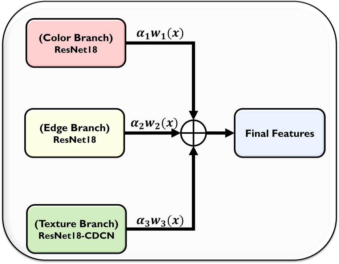
The novel proposed automatic adaptive weighted feature-fusion-based plant disease identification classifier is a 3-branch architecture, as illustrated in Figure 1. The first branch, namely, the color feature branch, contains the RGB values of the images (size of 256 × 256), which are passed as input to a ResNet-18 DNN and deep, robust features ( F 1 ) of size 512 × 7 × 7 are extracted from this branch. The second branch is the edge feature branch, in which the input is the image that contain the Sobel edge information. For generating the input for the edge branch, the RGB images are first converted into grayscale images and then the Sobel edge detection is applied.

Figure 1

The proposed network architecture: Color + edge + texture.

The Sobel edge information images are then passed into a ResNet-18 architecture and its deep, robust features ( F 2 ) of size 512 × 7 × 7 are extracted from this branch. The third branch is called the texture feature branch. It is created by replacing the traditional convolutional layers of ResNet-18 DNN with the newly introduced texture descriptor, Central Difference Convolutional layers. The RGB images are passed to this new ResNet-central difference convolution network (CDCN), and the deep, robust features ( F 3 ) of size 512 × 7 × 7 are extracted from this branch.

These features obtained from every branch are of size ( 512 × 7 × 7 ). For analyzing the contribution of each feature, some weights ( α n , where n = 1 , 2 , 3 ) are assigned to features obtained from each branch, which are achieved by multiplying the assigned weights to the features and creating the new features F 1 ′ , F 2 ′ , and F 3 ′ . These weighted features are summed up to create a combinational feature, i.e., F 4 .

The dimensionality of these F 4 features were too high, i.e., 1 , 536 × 7 × 7 . It is then reduced using two convolutional layers to suit the hardware compatibility. The new features F 6 obtained after two convolutions are of size 16 × 5 × 5 . The features are then flattened to a feature vector, F 7 of size 400 × 1 . These final features were passed to the fully connected layer and then to the SoftMax Layer for classification.

3.1 Extraction of texture features using CDCN

CDCN is a textural descriptor that provides texture difference information of an object by combining the pixel intensity value and its gradient information, as shown in Figure 2. CDCN helps to obtain the patterns’ essential and significant features by merging the intensity and gradient information. Unlike the textural description models based on vanilla convolution, it is more robust in model building. It provides extraordinary performance in extracting the features from fine-grained patterns captured in environments with diverse variations. The advantage of CDC over the traditional vanilla convolution is that without increasing any parameter, it can work in the place of vanilla convolution with the capability of generating models more robust than traditional ones [32].

Figure 2

CDC method.

The standard vanilla convolution used to extract features in CNNs can be represented as follows:

(5) M s + 1 ( f c ) = ∑ f l ∈ l w ( f l ) ( M s ( f c + f l ) − M s ( f c ) ) ,

where M s + 1 ( f c ) signifies the next level feature map extracted from the current feature map M s ( f c ) . f c carries the pixel value of the current feature map. l represents the local receptive field region to be operated. f l carries the pixel value of the local receptive field and enumerates through the kernel neighborhood. w is the weight used in the kernel.

The CDC and vanilla convolution are combined to become

(6) M s + 1 ( f c ) = ( 1 − σ ) ∑ f l ∈ l w ( f l ) M s ( f c + f l ) + σ ∑ f l ∈ l w ( f l ) ( M s ( f c + f l ) − M s ( f c ) ,

where σ parameter is used for the combination and σ ∈ [ 0 , 1 ] . The final generalized CDC equation can be expressed as follows [33]:

(7) M s + 1 ( f c ) = ∑ f l ∈ l w ( f l ) M s ( f c + f l ) − σ ∑ f l ∈ l w ( f l ) ( M s ( f l ) .

The ResNet–CDCN model integrates transfer learning and fine-tuning for an improved training experience. In this work, the CDC is used to replace all the convolutions in ResNet-18 architecture, as shown in Figure 3, due to its capability to avoid any additional parameters in the network while still providing a more robust textural description. The learning rate (LR) optimizer is also employed in training for optimizing the network.

Figure 3

Converting ResNet18 architecture to ResNet–CDCN.

4 Dataset description

The dataset used for this work is the publicly available dataset, the PlantVillage dataset [34]. The hugest dataset publicly available for plant disease identification tasks contains 53,606 color plant leaf images. This dataset has been used for the same task by many researchers [35,36,37,38,39]. The images are labelled with 38 classes, including healthy plant leaf images and plant leaf images of different types of diseases. The total number of plants used to create the dataset is 14. The resolution of these images is 256 × 256 pixels and are in JPEG format. Few samples from the dataset can be seen in Figure 4.

Figure 4

Sample images from the PlantVillage dataset for plant disease identification.

The images of healthy plant leaves possess uniform color, no abnormalities, or discoloration. On the other hand, the diseased plant leaf images exhibit symptoms like different color spots, lines and patches, and discolored, crumbled, and dead-looking parts of the leaves. These symptoms can be identified with the help of some manual experts.

5 Experimental setup and results

For the experimental setup, the parameters are fixed for all models. The database used contained 53,606 images in JPEG format. The resolution of the images is 256 × 256 pixels. The split to train the data is set to be 80:10:10, i.e., 80% data is used for training, 10% data is used for validation, and the rest of the 10% data is used for testing the system. The batch size and epochs are chosen to facilitate the system capacity, i.e., 8 and 15, respectively. The ADAM optimizer is used in the models for training. The initial LR is set to be 0.0001, and a learning rate optimizer is integrated to improve the accuracy. The period of LR decay is chosen to be 1, with the multiplicative factor of LR decay as 0.8. The execution environment of all the models is an NVIDIA Graphical Processing Unit, as summarized in Table 1.

5.2 Automatic weight updation mechanism (AWUM)

The AWUM [42] contains two steps: (1) Combining the three types of features that are good in extracting significant features, as shown in Figure 5. The color, edge, and texture features are chosen in this case. All these features perform well in the feature extraction procedure but contribute differently to the process. (2) Assigning different weights to the features and analyzing their individual, as well as the combinational, contribution can be beneficial for choosing the best features, reducing time consumption and redundant information that can help obtain better results in classifying the diseases in plants.

Figure 5

Automatic weight updation mechanism.

The features used, apart from the color images, are the images containing Sobel edge features and the texture features extracted by using the CDCN. The equation used for the AWUM can be expressed as follows [42]:

(8) W = ∑ i I α i w i ( x ) , ∑ i I α i = 0.25 , 0.4 , 0.5 , 0.6 , 0.75 , 1.0 ,

where α signifies the weight assigned to a feature. w i corresponds to the features, and W represents the output of the AWUM.

In this work, there is no need for human intervention to update the weights, but the system automatically updates the weights assigned to features to obtain the best value. This system updates the C value with the same mechanism as the system weights, i.e., the backpropagation algorithm. The α weights are appended to the list of system weights to get updated similarly. The weight α depends upon the contribution of the individual features used and gets automatically updated accordingly. This mechanism can wholly use each feature for the plant disease classification, and the best significant features can also be extracted. The final feature vector can be computed as follows:

(9) W = α 1 w 1 ( x ) + α 2 w 2 ( x ) + α 3 w 3 ( x ) α 1 + α 2 + α 3 = 1 ,

where α 1 , α 2 , and α 3 are the weight assigned to the individual features and used to compute the contribution of the features. The sum of the weights assigned to the features is kept such that the sum is 1.

5.4 Performance of color, edge, and texture information models

The RGB images are used for the color only and texture only models. The edge only model uses the Sobel edge images produced by applying the Sobel edge detector on RGB images, as represented in Figure 6.

Figure 6

Computation of features and classification based on individual feature models.

It has been observed that the color model produced the highest test accuracy, i.e., 99.108%, along with the highest precision, recall, F1, and AUC values: 98.894, 98.842, 98.861, and 99.995%, respectively. On the other hand, the second highest test accuracy is obtained using the texture only model, i.e., 94.423%, along with the highest precision, recall, F1, and AUC values: 93.286, 92.272, 92.679, and 99.909%, respectively. The least test accuracy is obtained using edge only model, i.e., 50.821%, along with the highest precision, recall, F1, and AUC values: 44.589, 36.889, 37.46, and 93.611%, respectively, as shown in Table 2. Loss/accuracy plots and confusion matrix plots for individual feature information models can be seen in Figure 7.

Table 2

Performance comparison of individual feature models based on highest accuracy achieved, precision, recall, F1 score, and AUC score

Model	Highest test accuracy	Precision	Recall	F1	AUC
Color only	99.108	98.894	98.842	98.861	99.995
Edge only	50.821	44.589	36.889	37.46	93.611
Texture only	94.423	93.286	92.272	92.679	99.909

Figure 7

Loss/accuracy plots for individual feature information models: (a) color only information model, (b) edge only information model, and (c) texture only information model.

Figure 8

Color + edge information model.

5.5 Performance of color + edge information model with different weight combinations

It has been observed that the best results of the proposed color + edge model (illustrated in Figure 8) are obtained when α 1 and α 2 are initialized to 0.5 and 0.5, respectively. It is further observed that the automatic weighting of α 1 and α 2 changes their values to 0.68 and 0.32, respectively, as shown in Table 3. This indicates that the model considers 68% of color features and 32% of edge features. The alpha initial values vs final values plot, loss/accuracy plots, confusion matrix plots for individual feature information models can be seen in Figures 9 and 10, respectively.

Figure 9

(a) Initial/final alpha value plot and (b) loss/accuracy plot for combinational feature information model: color + edge information model with best values ( α 1 = 50 % and α 2 = 50 % ).

Table 3

Performance comparison of color + edge information combinational model based on highest accuracy achieved, precision, recall, F1 score, and AUC score, with initial and final alpha values

Color + Edge
Initial alpha values		Final alpha values		Test accuracy	Precision	Recall	F1	AUC
α 1	α 2	α 1	α 2
0.5	0.5	0.68	0.32	99.248	98.829	98.852	98.826	99.983
0.6	0.4	0.74	0.26	99.02	98.547	98.522	98.525	99.994
0.4	0.6	0.60	0.40	99.195	98.991	98.856	98.914	99.998
0.75	0.25	0.82	0.18	99.02	98.647	98.486	98.559	99.99
0.25	0.75	0.47	0.53	99.108	98.801	98.865	98.826	99.993

Figure 10

Confusion matrix plot for combinational feature information model: Color + edge information model with best values ( α 1 = 50 % and α 2 = 50 % ).

Figure 11

Color + texture (CDC) information model.

Table 4

Performance comparison of color + texture information combinational model based on highest accuracy achieved, precision, recall, F1 score, and AUC score, with initial and final alpha values

Color + Texture
Initial alpha values		Final alpha values		Test accuracy	Precision	Recall	F1	AUC
α 1	α 2	α 1	α 2
0.5	0.5	0.62	0.38	99.23	99.154	99.144	99.146	99.997
0.6	0.4	0.70	0.30	98.986	98.877	98.803	98.836	99.992
0.4	0.6	0.48	0.52	99.195	99.067	98.894	98.977	99.996
0.75	0.25	0.86	0.14	99.073	98.968	98.787	98.868	99.996
0.25	0.75	0.35	0.65	99.073	98.831	98.641	98.731	99.993

5.6 Performance of the color + texture (CDC) information model with different weight combinations

It has been observed that the best results of the proposed color + texture model (illustrated in Figure 11) are obtained when α 1 and α 2 are initialized to 0.5 and 0.5, respectively. It is further observed that the automatic weighting of α 1 and α 2 changes their value to 0.62 and 0.38, respectively, as shown in Table 5. This indicates that the model considers 62% of color features and 38% of texture features. The alpha initial values vs final values plot, Loss/accuracy plots, and confusion matrix plots for individual feature information models can be seen in Figures 12 and 13, respectively (Table 4).

Figure 12

(a) Initial/final alpha value plot and (b) loss/accuracy plot for combinational feature information model: color + texture information model with best values ( α 1 = 100 % and α 2 = 100 % ).

Table 5

Performance comparison of edge + texture information combinational model based on highest accuracy achieved, precision, recall, F1 score, and AUC score, with initial and final alpha values

Edge + Texture
Initial alpha values		Final alpha values		Test accuracy	Precision	Recall	F1	AUC
α 1	α 2	α 1	α 2
0.5	0.5	0.47	0.53	90.594	88.841	86.956	87.562	99.81
0.6	0.4	0.54	0.46	89.683	86.648	85.706	86.025	99.73
0.4	0.6	0.42	0.58	91.59	90.139	89.671	89.831	99.836
0.75	0.25	0.65	0.35	90.052	87.378	86.563	86.818	99.754
0.25	0.75	0.33	0.67	91.241	89.977	87.965	88.803	99.839

Figure 13

Confusion matrix plot for combinational feature information model: Color + texture information model with best values ( α 1 = 100 % and α 2 = 100 % ).

Figure 14

Edge + texture (CDC) information model.

5.7 Performance of the edge + texture (CDC) information model with different weight combinations

It has been observed that the best results of the proposed edge + texture model (illustrated in Figure 14) are obtained when α 1 and α 2 are initialized to 0.4 and 0.6, respectively. It is further observed that the automatic weighting of α 1 and α 2 changes their value to 0.42 and 0.58, respectively, as shown in Table 6. This indicates that the model considers 42% of edge features and 58% of texture features. The alpha initial values vs final values plot, loss/accuracy plots, and confusion matrix plots for individual feature information models can be seen in Figures 15 and 16, respectively.

Figure 15

(a) Initial/final alpha value plot and (b) loss/accuracy plot for combinational feature information model: edge + texture information model with best values ( α 1 = 40 % and α 2 = 60 % ).

Table 6

Performance comparison of Color + edge + texture information combinational model based on highest accuracy achieved, precision, recall, F1 score, and AUC score, with initial and final alpha values

Color + Edge + Texture
Initial alpha values			Final alpha values			Test accuracy	Precision	Recall	F1	AUC
α 1	α 2	α 3	α 1	α 2	α 3
0.33	0.33	0.33	0.54	0.23	0.23	99.09	98.995	98.905	98.942	99.99
0.50	0.25	0.25	0.71	0.19	0.10	99.09	98.839	98.865	98.836	99.994
0.25	0.50	0.25	0.49	0.37	0.14	99.108	98.908	98.777	98.826	99.997
0.25	0.25	0.50	0.41	0.17	0.42	99.23	98.93	99123	99.02	99.996
0.60	0.20	0.20	0.74	0.16	0.10	99.003	98.917	98.511	98.698	99.996
0.20	0.60	0.20	0.43	0.44	0.13	99.16	98.948	98.975	98.955	99.997
0.20	0.20	0.60	0.34	0.16	0.50	99.143	98.974	98.889	98.926	99.987
0.70	0.15	0.15	0.82	0.11	0.06	99.055	98.676	98.634	98.64	99.995
0.15	0.70	0.15	0.38	0.50	0.13	99.213	99.094	98.839	98.956	99.998
0.15	0.15	0.70	0.30	0.13	0.56	98.898	98.577	98.553	98.554	99.995

Figure 16

Confusion matrix plot for combinational feature information model: edge + texture information model with best values ( α 1 = 40 % and α 2 = 60 % ).

Figure 17

Color + edge + texture (CDC) information model.

5.8 Performance of color + edge + texture (CDC) information model with different weight combinations

It has been observed that the best results of the proposed color + edge + texture model (illustrated in Figure 17) are obtained when α 1 , α 2 , and α 3 are initialized to 0.25, 0.25, and 0.50, respectively. It is further observed that the automatic weighting of α 1 , α 2 , and α 3 changes their value to 0.41, 0.17, and 0.42, respectively, as shown in Table 7. This indicates that the model considers 41% of color features, 17% of edge features, and 42% of texture features. The alpha initial values vs final values plot, loss/accuracy plots, and confusion matrix plots for individual feature information models can be seen in Figure 18.

Figure 18

Plots for combinational feature information model: color + edge + texture model with best values ( α 1 = 25 % , α 2 = 25 % , and α 3 = 50 % ). (a) Initial/final alpha value plot, (b) loss/accuracy plot, and (c) confusion matrix plot.

Table 7

Comparison between all the models with their best-obtained values: Highest accuracy provided by color + texture model with best values ( α 1 = 50% and α 2 = 50%)

Model	Best alpha values			Highest test accuracy	Precision	Recall	F1	AUC
	α 1	α 2	α 3
Color only	—			99.108	98.894	98.842	98.861	99.995
Edge only	—			50.821	44.589	36.889	37.46	93.611
Texture only				94.423	93.286	92.272	92.679	99.909
Color + edge	0.5	0.5	—	99.248	98.829	98.852	98.826	99.983
Color + texture	0.5	0.5	—	99.230	98.98	99.1	99	100
Edge + texture	0.4	0.6	—	91.59	90.139	89.671	89.831	99.836
Color + edge + texture	0.25	0.25	0.5	99.230	98.93	99123	99.02	99.996

Figure 19

Plots for (a) highest accuracy achieved, (b) precision, (c) recall, (d) F1 score, and (e) AUC for all models.

It is noticed that the color + texture model outperformed all other models with the highest accuracy of 99.23%, as shown in Table 8. The precision, recall, F1 score, and AUC are obtained to be 98.98, 99.10, 99, and 100%, respectively, as represented in Figure 19.

Table 8

Comparison of existing approaches and the proposed approach

Approaches	Accuracy (%)
Hu et al. [45]	91.22
Chen et al. [46]	92
Ma et al. [47]	93
Agarwal et al. [48]	94
Alehegn [49]	95.63
Gao and Lin [50]	96.02
Bin Tahir et al. [51]	97
Kaur et al. [52]	97.7
Sethy et al. [53]	97.96
Waheed et al. [54]	98.06
The proposed approach	99.230

Figure 20

Comparison of existing approaches and the novel proposed approach.

5.9 Performance comparison of traditional plant disease identification approaches and the proposed approach

In this work, the test accuracy is the performance metric for comparing the traditional approaches for plant disease classification and the proposed novel automatic adaptive weighted features-fusion-based approach for plant disease identification. The traditional techniques for plant disease classification provided the accuracy as high as 91.22, 92, 93, 94, 95.63, 96.02, 97, 97.7, 97.96, and 98.06%, respectively as shown in Table 8. The proposed novel weighted features-fusion-based approach performed exhaustively and provided the highest accuracy of 99.230%, as illustrated in Figure 20.

Figure 21

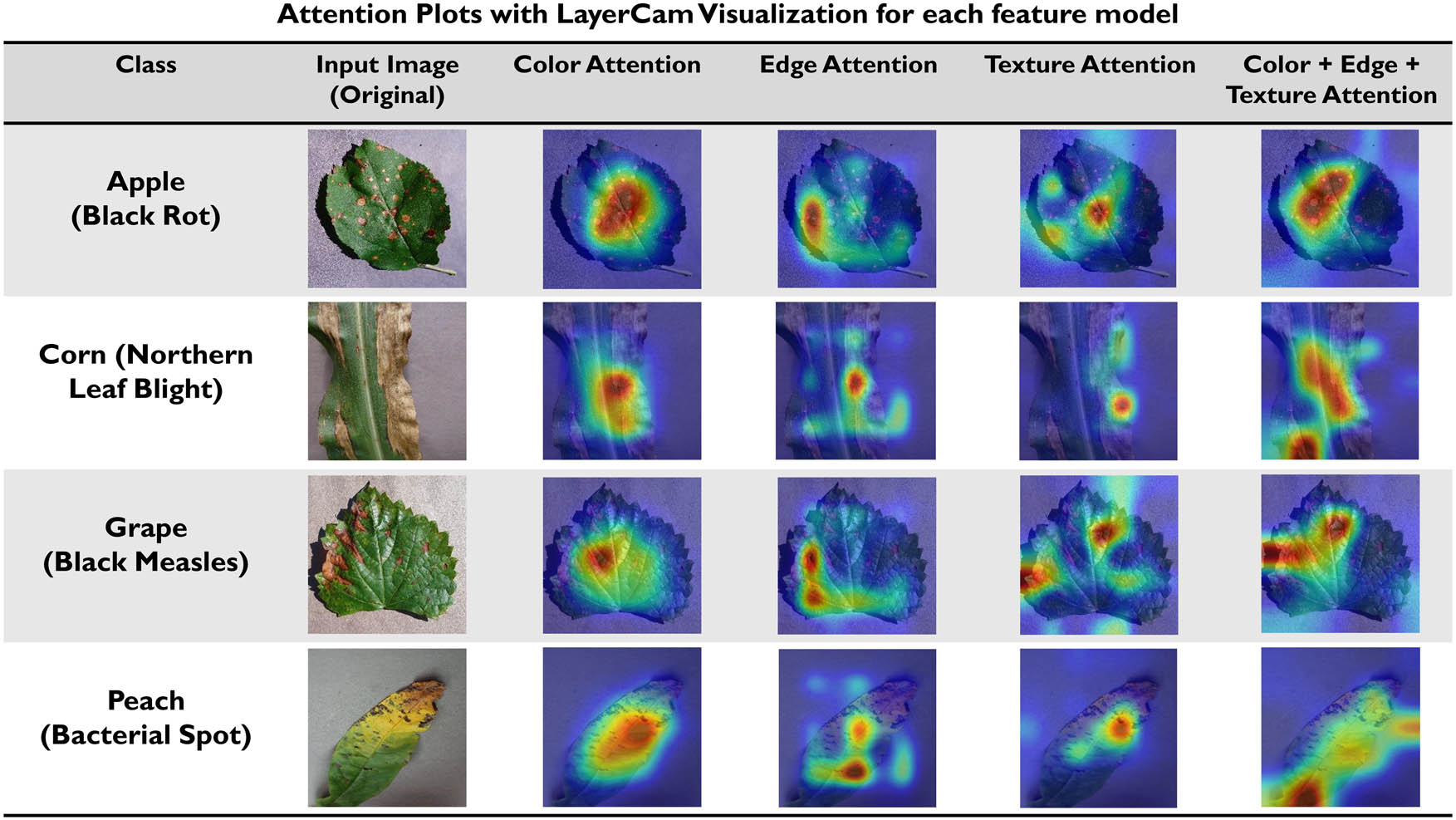
Attention plots with LayerCAM visualization for each feature model.

6 Visualization of results with LayerCAM for different feature attentions

Zhou introduced the idea of visualizing the features via class activation maps, which proposed the concept of CAMs, i.e., Class Activation Maps [48]. These CAMs were created using the neural network structure in which the global average pooling layer replaced the fully connected layer. Various methods were introduced in past years to generate class activation maps. They could able to locate the target feature regions excellently. Still, the problem that has been found so common among all these methods is that they utilized the final convolutional layer of CNN to create CAMs. The issue with relying on a final convolutional layer of CNN is that it has a low spatial resolution and hence can trace only the coarse regions [49], which limits the performance of the CAM methods.

LayerCAM is convenient with the standard CNN-based image classifiers without altering the network architectures and weights obtained from backpropagation. The LayerCAM attention method was introduced by Jiang. LayerCAM does not uses the final convolutional layer of CNN but also utilizes different shallower layers of the CNN to create effective class activation maps to obtain more fine-grain features and to locate the target effectively. The attention plots or class activation maps of all three models, color model, edge model, and the proposed color + edge + texture model, utilized in this work, can be seen in Figure 21.

7 Discussion

In this work, we introduced a novel automatic adaptive weighted fusion of features-based approach for plant disease identification. The proof of the efficiency of the proposed approach can be seen in Tables 7 and 8. The key insights of the proposed approach are described as follows:

1. The experiments examined the proposed approach in every aspect, i.e., in terms of test accuracy, F1 score, precision, recall, and AUC score.

2. The developed approach provided the highest accuracy among all the existing feature-fusion-based approaches, i.e., 99.230%

3. Out of the total 53,606 images, the proposed feature-fusion-based approach classified 53,193 images correctly, and only 413 images were misclassified.

4. The proposed approach provided significant insight into the contribution of the features used, i.e., the color features and the texture features contributed the highest in the classification of the images, even contributed equally. On the other hand, edge features contributed negligibly to the process.

Apart from the several advantages, this approach also has some limitations. First, the images used for the experiments were captured in an environment with no chance of illumination variation, which eased the classification process. The system could not get the opportunity to face the challenge of tackling illumination variations. Another limitation is that the leaf images of the dataset contain one type of disease per leaf. In real-world scenarios, the problem of disease identification is much more complex because the leaves may contain multiple diseases per leaf. In future, the system will be improvised to work for the leaf images containing various illumination variations and with multiple disease symptoms.

8 Conclusion

Integrating the color, edge, and texture features, a novel 3-branch classifier for plant disease classification has been proposed. The proposed classifier can classify between 38 classes of 14 different plants. A newly introduced texture extraction method is used for extracting the prominent texture from the plant leaves, i.e., CDCN. The features are trained using ResNet-18 with an AWUM for automatically adjusting the weights in DNN and analyzing each feature’s contribution to achieving the highest classification accuracy. The individual features, as well as the combinational features, are analyzed by performing various types of experiments. The highest accuracy is achieved with a 50% contribution of color features and 50% of texture features. The proposed classifier outperformed the existing feature-fusion-based approaches for plant disease identification.

References

[1] Richard B, Qi A, Fitt BDL. Control of crop diseases through integrated crop management to deliver climate-smart farming systems for low- and high-input crop production. Plant Pathol. Jan. 2022;71(1):187–206. 10.1111/PPA.13493.Search in Google Scholar
[2] Fry WE, Birch PRJ, Judelson HS, Grünwald NJ, Danies G, Everts KL, et al. Five reasons to consider phytophthora infestans a reemerging pathogen. Phytopathology. Jul. 2015;105(7):966–81. 10.1094/PHYTO-01-15-0005-FI/ASSET/IMAGES/LARGE/PHYTO-01-15-0005-FI_F9.JPEG.Search in Google Scholar
[3] Padmanabhan SY. Gt Bengal Famine. Annu Rev Phytopathol. 1973;11(1):11–24. 10.1146/ANNUREV.PY.11.090173.000303. http://dx.doi.org/10.1146/annurev.py.11.090173.000303.Search in Google Scholar
[4] Rajarajeswari NVL, Muralidharan K. Assessments of farm yield and district production loss from bacterial leaf blight epidemics in rice. Crop Prot. Mar. 2006;25(3):244–52. 10.1016/j.cropro.2005.04.013.Search in Google Scholar
[5] Akrofi AY, Amoako-Atta I, Assuah M, Asare EK. Black pod disease on cacao (Theobroma cacao, L) in Ghana: Spread of Phytophthora megakarya and role of economic plants in the disease epidemiology. Crop Prot. Jun. 2015;72:66–75. 10.1016/j.cropro.2015.01.015.Search in Google Scholar
[6] Katewa R, Mathur K, Bunker RN. Assessment of losses in sorghum due to target leaf spot (Bipolaris sorghicola) at varying disease severity levels. Indian Phytopathology. 2006;59(2):237.Search in Google Scholar
[7] Lowe A, Harrison N, French AP. Hyperspectral image analysis techniques for the detection and classification of the early onset of plant disease and stress. Plant Methods. Oct. 2017;13(1):1–12. 10.1186/S13007-017-0233-Z/TABLES/2.Search in Google Scholar
[8] Kirti K, Rajpal N. Black rot disease detection in grape plant (vitis vinifera) using colour based segmentation machine learning. Proceedings - IEEE 2020 2nd International Conference on Advances in Computing, Communication Control and Networking. ICACCCN 2020; Dec. 2020. p. 976–9. 10.1109/ICACCCN51052.2020.9362812.Search in Google Scholar
[9] Kirti K, Rajpal N, Yadav J. A novel DWT and deep learning based feature extraction technique for plant disease identification. Proceedings of Second Doctoral Symposium on Computational Intelligence: DoSCI 2021 2022. Springer Singapore; 2022. p. 355–67. 10.1007/978-981-16-3346-1_29.Search in Google Scholar
[10] Kirti K, Rajpal N, Arora M. Comparison of texture based feature extraction techniques for detecting leaf scorch in strawberry plant (Fragaria × Ananassa). Lecture Notes in Electrical Engineering. Singapore: Springer; Vol. 698; 2021. p. 659–70p. 10.1007/978-981-15-7961-5_63.Search in Google Scholar
[11] Kirti K, Rajpal N, Yadav J. Black measles disease identification in grape plant (vitis vinifera) using deep learning. 2021 International Conference on Computing, Communication, and Intelligent Systems (ICCCIS); Feb. 2021. p. 97–101. 10.1109/ICCCIS51004.2021.9397205.Search in Google Scholar
[12] Wäldchen J, Mäder P. Machine learning for image based species identification. Methods Ecol Evol. Nov. 2018;9(11):2216–25. 10.1111/2041-210X.13075.Search in Google Scholar
[13] Gaddam DKR, Ansari MD, Vuppala S, Gunjan VK, Sati MM. A performance comparison of optimization algorithms on a generated dataset. Lect Notes Electr Eng. 2022;783:1407–15. 10.1007/978-981-16-3690-5_135/COVER.Search in Google Scholar
[14] Bhat SS, Selvam V, Ansari GA, Ansari MD, Rahman MH. Prevalence and early prediction of diabetes using machine learning in North Kashmir: A case study of district Bandipora. Comput Intell Neurosci. 2022;2022:1–12. 10.1155/2022/2789760.Search in Google Scholar PubMed PubMed Central
[15] Goel AK, Chakraborty R, Agarwal M, Ansari MD, Gupta SK, Garg D. Profit or loss: A long short term memory based model for the prediction of share price of DLF group in India. Proc. 2019 IEEE 9th International Conference Advanced Comput. IACC 2019; Dec. 2019. p. 120–4. 10.1109/IACC48062.2019.8971601.Search in Google Scholar
[16] Gunjan VK, Kumar S, Ansari MD, Vijayalata Y. Prediction of agriculture yields using machine learning algorithms. Lect Notes Netw Syst. 2022;237:17–26. 10.1007/978-981-16-6407-6_2/COVER.Search in Google Scholar
[17] Sethi K, Jaiswal V, Ansari MD. Machine learning based support system for students to select stream (Subject). Recent Adv Comput Sci Commun. Nov. 2018;13(3):336–44. 10.2174/2213275912666181128120527.Search in Google Scholar
[18] Jaiswal A, Krishnama Raju A, Deb S. Facial emotion detection using deep learning. 2020 International Conference Emerging Technologies. INCET 2020; Jun. 2020. 10.1109/INCET49848.2020.9154121.Search in Google Scholar
[19] Gaddam DKR, Ansari MD, Vuppala S. On sudoku problem using deep learning and image processing technique. Lect Notes Electr Eng. 2021;698:1405–17. 10.1007/978-981-15-7961-5_128/COVER.Search in Google Scholar
[20] Kabbai L, Abdellaoui M, Douik A. Image classification by combining local and global features. Vis Comput. May 2019;35(5):679–93. 10.1007/S00371-018-1503-0/TABLES/8.Search in Google Scholar
[21] Ping Tian D. A review on image feature extraction and representation techniques. Int J Multimed Ubiquitous Eng. 2013;8(4):385–96.Search in Google Scholar
[22] Mutlag WK, Ali SK, Aydam ZM, Taher BH. Feature extraction methods: A Review. J Physics: Conf Ser. Aug. 2020;1591:1. 10.1088/1742-6596/1591/1/012028.Search in Google Scholar
[23] Bankar S, Dube A, Kadam P, Deokule S. Plant disease detection techniques using canny edge detection & color histogram in image processing. Int J Comput Sci Inf Technol. 2014;5(2):1165–8, [Online] www.ijcsit.com.Search in Google Scholar
[24] Dubey SR, Jalal AS. Apple disease classification using color, texture and shape features from images. Signal, Image Video Process. Jul. 2016;10(5):819–26. 10.1007/s11760-015-0821-1.Search in Google Scholar
[25] Al-Saddik H, Laybros A, Billiot B, Cointault F. Using image texture and spectral reflectance analysis to detect yellowness and esca in grapevines at leaf-level. Remote Sens. 2018;10(4):618. 10.3390/RS10040618.Search in Google Scholar
[26] Naeem S, Ali A, Chesneau C, Tahir MH, Jamal F, Sherwani RAK, et al. The classification of medicinal plant leaves based on multispectral and texture feature using machine learning approach. Agronomy. 2021;11(2):263. 10.3390/AGRONOMY11020263. Jan. 2021.Search in Google Scholar
[27] Khan SI, Shahrior A, Karim R, Hasan M, Rahman A. MultiNet: A deep neural network approach for detecting breast cancer through multi-scale feature fusion. J King Saud Univ - Comput Inf Sci. Sep. 2022;34(8):6217–28. 10.1016/j.jksuci.2021.08.004.Search in Google Scholar
[28] Almaraz-Damian JA, Ponomaryov V, Sadovnychiy S, Castillejos-Fernandez H. Melanoma and nevus skin lesion classification using handcraft and deep learning feature fusion via mutual information measures. Entropy. Apr. 2020;22(4):1–23. 10.3390/E22040484.Search in Google Scholar PubMed PubMed Central
[29] Sharif M, Amin J, Nisar MW, Anjum MA, Muhammad N, Ali Shad S. A unified patch based method for brain tumor detection using features fusion. Cogn Syst Res. Jan. 2020;59:273–86. 10.1016/j.cogsys.2019.10.001.Search in Google Scholar
[30] Nur-a-alam M, Ahsan MA, Based J, Haider, Kowalski M. COVID-19 detection from chest X-ray images using feature fusion and deep learning. Sensors. Feb. 2021;21(4):1–30. 10.3390/s21041480.Search in Google Scholar PubMed PubMed Central
[31] Yang F, Ma Z, Xie M. Image classification with superpixels and feature fusion method. J Electron Sci Technol. Mar. 2021;19(1):100096. 10.1016/J.JNLEST.2021.100096.Search in Google Scholar
[32] Yang J, Li A, Xiao S, Lu W, Gao X. MTD-Net: Learning to detect deepfakes images by multi-scale texture difference. IEEE Trans Inf Forensics Secur. 2021;16:4234–45. 10.1109/TIFS.2021.3102487.Search in Google Scholar
[33] Yu Z, Zhao C, Wang Z, Qin Y, Su Z, Li X, et al. Searching Central Difference Convolutional Networks for Face Anti-Spoofing. Accessed: Aug. 05, 2022. [Online]. https://github.com/ZitongYu/CDCN.Search in Google Scholar
[34] GitHub - spMohanty/PlantVillage-Dataset: Dataset of diseased plant leaf images and corresponding labels. https://github.com/spMohanty/PlantVillage-Dataset (accessed Jan. 13, 2021).Search in Google Scholar
[35] Haque M, Marwaha S, Deb CK, Nigam S, Arora A, Hooda KS, et al. Deep learning-based approach for identification of diseases of maize crop. Sci Rep. 2012;12(1):1–14. 10.1038/s41598-022-10140-z.Search in Google Scholar PubMed PubMed Central
[36] Detection of disease in tomato plant using Deep Learning Techniques | International Journal of Modern Agriculture. http://www.modern-journals.com/index.php/ijma/article/view/374 (accessed Aug. 05, 2022).Search in Google Scholar
[37] Deep D, Craze HA, Pillay N, Joubert F, Berger DK. Deep learning diagnostics of gray leaf spot in maize under mixed disease field conditions. Plants. Jul. 2022;11(15):1942. 10.3390/PLANTS11151942.Search in Google Scholar
[38] Mohameth F, Bingcai C, Sada KA, Mohameth F, Bingcai C, Sada KA. plant disease detection with deep learning and feature extraction using plant village. J Comput Commun. Jun. 2020;8(6):10–22. 10.4236/JCC.2020.86002.Search in Google Scholar
[39] Barbedo JGA. Plant disease identification from individual lesions and spots using deep learning. Biosyst Eng. Apr. 2019;180:96–107. 10.1016/J.BIOSYSTEMSENG.2019.02.002.Search in Google Scholar
[40] Smith LN. Cyclical learning rates for training neural networks. Proc. - 2017 IEEE Winter Conf. Appl. Comput. Vision, WACV 2017. Jun. 2015. p. 464–72. 10.48550/arxiv.1506.01186.Search in Google Scholar
[41] StepLR – PyTorch 1.11.0 documentation. https://pytorch.org/docs/stable/generated/torch.optim.lr_scheduler.StepLR.html (accessed Jun. 27, 2022).Search in Google Scholar
[42] Wang J, Ni Q, Liu G, Luo X, Jha SK. Image splicing detection based on convolutional neural network with weight combination strategy. J Inf Secur Appl. Oct. 2020;54:1–8. 10.1016/j.jisa.2020.102523.Search in Google Scholar
[43] Shorten C, Khoshgoftaar TM. A survey on Image Data Augmentation for Deep Learning. J Big Data. Dec. 2019;6:1. 10.1186/s40537-019-0197-0.Search in Google Scholar
[44] Perez L, Wang J. The Effectiveness of Data Augmentation in Image Classification using Deep Learning. Dec. 2017, [Online]. http://arxiv.org/abs/1712.04621.Search in Google Scholar
[45] Hu G, Wang H, Zhang Y, Wan M. Detection and severity analysis of tea leaf blight based on deep learning. Comput Electr Eng. Mar. 2021;90:1–15. 10.1016/j.compeleceng.2021.107023.Search in Google Scholar
[46] Chen J, Chen J, Zhang D, Sun Y, Nanehkaran YA. Using deep transfer learning for image-based plant disease identification. Comput Electron Agric. Jun. 2020;173:1–11. 10.1016/j.compag.2020.105393.Search in Google Scholar
[47] Ma J, Du K, Zheng F, Zhang L, Gong Z, Sun Z. A recognition method for cucumber diseases using leaf symptom images based on deep convolutional neural network. Comput Electron Agric. Nov. 2018;154:18–24. 10.1016/j.compag.2018.08.048.Search in Google Scholar
[48] Agarwal M, Bohat VK, Ansari MD, Sinha A, Gupta SK, Garg D. A convolution neural network based approach to detect the disease in corn crop. Proc. 2019 IEEE 9th Int. Conf. Adv. Comput. IACC 2019; Dec. 2019. p. 176–81. 10.1109/IACC48062.2019.8971602.Search in Google Scholar
[49] Alehegn E. Ethiopian maize diseases recognition and classification using support vector machine. Int J Comput Vis Robot. 2019;9(1):90–109. 10.1504/IJCVR.2019.098012.Search in Google Scholar
[50] Gao L, Lin X. Fully automatic segmentation method for medicinal plant leaf images in complex background. Comput Electron Agric. Sep. 2019;164. 10.1016/j.compag.2019.104924.Search in Google Scholar
[51] Bin Tahir M, Khan MA, Javed K, Kadry S, Zhang Y, Akram T, et al. Recognition of apple leaf diseases using deep learning and variances-controlled features reduction. Microprocess Microsyst. Jan. 2021;104027. 10.1016/j.micpro.2021.104027.Search in Google Scholar
[52] Kaur A, Singh S, Nayyar A, Singh P. Classification of wheat seeds using image processing and fuzzy clustered random forest. Int J Agric Resour Gov Ecol. 2020;16(2):1. 10.1504/ijarge.2020.10030235.Search in Google Scholar
[53] Sethy PK, Barpanda NK, Rath AK, Behera SK. Deep feature based rice leaf disease identification using support vector machine. Comput Electron Agric. Aug. 2020;175:1–9. 10.1016/j.compag.2020.105527.Search in Google Scholar
[54] A Waheed, M Goyal, D Gupta, A Khanna, AE Hassanien, HM Pandey. An optimized dense convolutional neural network model for disease recognition and classification in corn leaf. Comput Electron Agric, Aug. 2020;175:1–11, 10.1016/j.compag.2020.105456.Search in Google Scholar
© 2023 the author(s), published by De Gruyter
This work is licensed under the Creative Commons Attribution 4.0 International License.
Articles in the same Issue
- Research Articles
- Salp swarm and gray wolf optimizer for improving the efficiency of power supply network in radial distribution systems
- Deep learning in distributed denial-of-service attacks detection method for Internet of Things networks
- On numerical characterizations of the topological reduction of incomplete information systems based on evidence theory
- A novel deep learning-based brain tumor detection using the Bagging ensemble with K-nearest neighbor
- Detecting biased user-product ratings for online products using opinion mining
- Evaluation and analysis of teaching quality of university teachers using machine learning algorithms
- Efficient mutual authentication using Kerberos for resource constraint smart meter in advanced metering infrastructure
- Recognition of English speech – using a deep learning algorithm
- A new method for writer identification based on historical documents
- Intelligent gloves: An IT intervention for deaf-mute people
- Reinforcement learning with Gaussian process regression using variational free energy
- Anti-leakage method of network sensitive information data based on homomorphic encryption
- An intelligent algorithm for fast machine translation of long English sentences
- A lattice-transformer-graph deep learning model for Chinese named entity recognition
- Robot indoor navigation point cloud map generation algorithm based on visual sensing
- Towards a better similarity algorithm for host-based intrusion detection system
- A multiorder feature tracking and explanation strategy for explainable deep learning
- Application study of ant colony algorithm for network data transmission path scheduling optimization
- Data analysis with performance and privacy enhanced classification
- Motion vector steganography algorithm of sports training video integrating with artificial bee colony algorithm and human-centered AI for web applications
- Multi-sensor remote sensing image alignment based on fast algorithms
- Replay attack detection based on deformable convolutional neural network and temporal-frequency attention model
- Validation of machine learning ridge regression models using Monte Carlo, bootstrap, and variations in cross-validation
- Computer technology of multisensor data fusion based on FWA–BP network
- Application of adaptive improved DE algorithm based on multi-angle search rotation crossover strategy in multi-circuit testing optimization
- HWCD: A hybrid approach for image compression using wavelet, encryption using confusion, and decryption using diffusion scheme
- Environmental landscape design and planning system based on computer vision and deep learning
- Wireless sensor node localization algorithm combined with PSO-DFP
- Development of a digital employee rating evaluation system (DERES) based on machine learning algorithms and 360-degree method
- A BiLSTM-attention-based point-of-interest recommendation algorithm
- Development and research of deep neural network fusion computer vision technology
- Face recognition of remote monitoring under the Ipv6 protocol technology of Internet of Things architecture
- Research on the center extraction algorithm of structured light fringe based on an improved gray gravity center method
- Anomaly detection for maritime navigation based on probability density function of error of reconstruction
- A novel hybrid CNN-LSTM approach for assessing StackOverflow post quality
- Integrating k-means clustering algorithm for the symbiotic relationship of aesthetic community spatial science
- Improved kernel density peaks clustering for plant image segmentation applications
- Biomedical event extraction using pre-trained SciBERT
- Sentiment analysis method of consumer comment text based on BERT and hierarchical attention in e-commerce big data environment
- An intelligent decision methodology for triangular Pythagorean fuzzy MADM and applications to college English teaching quality evaluation
- Ensemble of explainable artificial intelligence predictions through discriminate regions: A model to identify COVID-19 from chest X-ray images
- Image feature extraction algorithm based on visual information
- Optimizing genetic prediction: Define-by-run DL approach in DNA sequencing
- Study on recognition and classification of English accents using deep learning algorithms
- Review Articles
- Dimensions of artificial intelligence techniques, blockchain, and cyber security in the Internet of medical things: Opportunities, challenges, and future directions
- A systematic literature review of undiscovered vulnerabilities and tools in smart contract technology
- Special Issue: Trustworthy Artificial Intelligence for Big Data-Driven Research Applications based on Internet of Everythings
- Deep learning for content-based image retrieval in FHE algorithms
- Improving binary crow search algorithm for feature selection
- Enhancement of K-means clustering in big data based on equilibrium optimizer algorithm
- A study on predicting crime rates through machine learning and data mining using text
- Deep learning models for multilabel ECG abnormalities classification: A comparative study using TPE optimization
- Predicting medicine demand using deep learning techniques: A review
- A novel distance vector hop localization method for wireless sensor networks
- Development of an intelligent controller for sports training system based on FPGA
- Analyzing SQL payloads using logistic regression in a big data environment
- Classifying cuneiform symbols using machine learning algorithms with unigram features on a balanced dataset
- Waste material classification using performance evaluation of deep learning models
- A deep neural network model for paternity testing based on 15-loci STR for Iraqi families
- AttentionPose: Attention-driven end-to-end model for precise 6D pose estimation
- The impact of innovation and digitalization on the quality of higher education: A study of selected universities in Uzbekistan
- A transfer learning approach for the classification of liver cancer
- Review of iris segmentation and recognition using deep learning to improve biometric application
- Special Issue: Intelligent Robotics for Smart Cities
- Accurate and real-time object detection in crowded indoor spaces based on the fusion of DBSCAN algorithm and improved YOLOv4-tiny network
- CMOR motion planning and accuracy control for heavy-duty robots
- Smart robots’ virus defense using data mining technology
- Broadcast speech recognition and control system based on Internet of Things sensors for smart cities
- Special Issue on International Conference on Computing Communication & Informatics 2022
- Intelligent control system for industrial robots based on multi-source data fusion
- Construction pit deformation measurement technology based on neural network algorithm
- Intelligent financial decision support system based on big data
- Design model-free adaptive PID controller based on lazy learning algorithm
- Intelligent medical IoT health monitoring system based on VR and wearable devices
- Feature extraction algorithm of anti-jamming cyclic frequency of electronic communication signal
- Intelligent auditing techniques for enterprise finance
- Improvement of predictive control algorithm based on fuzzy fractional order PID
- Multilevel thresholding image segmentation algorithm based on Mumford–Shah model
- Special Issue: Current IoT Trends, Issues, and Future Potential Using AI & Machine Learning Techniques