Endpoint carbon content and temperature prediction model in BOF steelmaking based on posterior probability and intra-cluster feature weight online dynamic feature selection

Haodong Wang; Hui Liu; FuGang Chen; Heng Li; XiaoJun Xue

doi:10.1515/htmp-2024-0067

Artikel Open Access

Endpoint carbon content and temperature prediction model in BOF steelmaking based on posterior probability and intra-cluster feature weight online dynamic feature selection

Haodong Wang , Hui Liu , FuGang Chen , Heng Li und XiaoJun Xue

Veröffentlicht/Copyright: 16. Januar 2025

Veröffentlicht von

Veröffentlichen auch Sie bei De Gruyter Brill

Manuskript einreichen Informationen für Autor*innen

Aus der Zeitschrift High Temperature Materials and Processes Band 44 Heft 1

Abstract

A posterior probability and intra-cluster feature weight online dynamic feature selection algorithm is proposed to address the issues of high dimensionality and high volatility of data in the basic oxygen furnace (BOF) steelmaking production process. First, a genetic algorithm with fixed feature space dimensions is introduced, which narrows the solution space by predefining the number of selected features, thereby enhancing the stability of feature selection. Second, the posterior probability of samples and intra-cluster feature weights are used to weigh and calculate the feature importance of the current sample, obtaining the optimal features that align with the current operating conditions. Finally, the dynamically selected features are used in a regression model to predict the carbon content and temperature of the BOF steelmaking process data. Simulations of actual BOF steelmaking process data showed that the prediction accuracy was 86% within a carbon content error range of 0.02, and 88% within a temperature error range of 10°C.

Keywords: BOF steelmaking; soft sensor; online dynamic feature selection algorithm; genetic algorithm

1 Introduction

The iron and steel industry plays an indispensable role in the industrialization process and the economic growth of a country [1,2]. The basic oxygen furnace (BOF) steelmaking method is the primary technological method used for steel production [3,4]. In the BOF process, pig iron and various raw materials are introduced, initiating a series of complex physical and chemical reactions that result in the production of high-quality steel. In the process of BOF steelmaking, the control of carbon content and temperature of liquid steel in the molten pool is the main basis for the judgment of the endpoint of the BOF steelmaking production process [5,6]. Therefore, realizing the accurate prediction of carbon content and temperature at the end of the BOF is a powerful means to improve the quality and production efficiency of BOF steelmaking. It is a non-negligible link to realize energy saving and emission reduction and to improve the economic efficiency of steel mills.

Currently, the endpoint prediction of BOF steelmaking mainly employs two methods: contact and non-contact [7]. Contact methods include the sublance detection method [8] and furnace gas analysis [9]. However, due to issues such as short sensor lifespan and lagging furnace gas analysis, this method is not suitable for small- and medium-sized enterprises. Non-contact methods [10] include spectrophotometry [11] and flame texture recognition method [12], which mimic workers’ observation of flames to determine carbon content and temperature. However, there are issues with low spectral quality and the influence of flame characteristics on accuracy with changing conditions.

In recent years, data-driven soft sensor methods [13] have often been used to solve problems in complex industrial processes where some variables are difficult to measure. There is a correlation between the carbon content and temperature in the molten pool during the production process of BOF steelmaking and the characteristics of the various raw materials added to the steelmaking process, such as the amount of oxygen blown and the total of transferred. By using these auxiliary variables to construct soft sensor models, predicting carbon content and temperature in the molten pool can effectively improve smelting efficiency.

Current mainstream soft sensor regression prediction models mainly include three methods: just-in-time learning (JITL) [14], deep learning [15], and ensemble learning [16]. Regardless of the soft sensor modeling and prediction method used, accuracy is highly dependent on the input features. In recent years, the dimensionality of process data has significantly expanded due to the increased number of sensors. However, in predicting endpoint carbon content and temperature in the BOF steelmaking process, traditional methods often utilize all available process data features as inputs for building predictive models. Direct prediction approaches that do not incorporate feature selection can lead to problems such as model overfitting, inefficient use of computational resources, the curse of dimensionality, feature redundancy, reduced interpretability, and susceptibility to data noise. Therefore, feature selection is both critical and challenging for achieving more accurate regression modeling.

Feature selection is generally categorized into two types: wrapper [17] and filter [18]. Wrapper feature selection evaluates the effectiveness of feature subsets using machine learning models, treating feature selection as an optimization problem and determining the optimal feature combination by training and evaluating the model’s performance. Although wrapper feature selection can effectively improve model performance, it incurs high computational costs as it requires retraining the model for each feature subset. Filter feature selection, on the other hand, evaluates feature independence and importance based on statistical properties or heuristic criteria, selecting features with high informational value by computing statistical measures between features and the target variable. Filter feature selection is computationally efficient as it does not rely on model training but may overlook interactions between features. Maleki et al. [19] proposed using a genetic algorithm (GA) for feature selection in the BOF steelmaking process data to address redundancy and identify features most relevant to the final carbon content and temperature. However, the high dimensionality of the data results in an extensive solution space for the GA, leading to unstable feature selection and a tendency to become trapped in local optima. Asghari et al. [20] proposed a principal component analysis-based feature selection approach utilizing statistical information. This method selects features based on mutual information between features and labels, and its advantage is that it does not consider subsequent learners. However, due to the nonlinearity, volatility, and multi-condition characteristics inherent in BOF steelmaking data, mutual information alone frequently proves inadequate in capturing the relevant interdependencies between features and labels and does not account for feature interrelationships. Chamlal et al. [21] proposed a hybrid feature selection algorithm that integrates filtering and wrapper methods. This method first uses statistical information to select the most relevant features and then uses graph theory to perform WRAPPER feature selection by considering feature relationships. Hermo et al. [22] proposed the joint minimum redundancy maximum relevance algorithm, which effectively addresses the feature interaction problem by dynamically accounting for changes in the information between features during feature selection. This approach also enables better feature selection in a joint learning environment with heterogeneous data. However, as a filter-based feature selection algorithm, this method exhibits high complexity and computational demands; yet, it does not achieve the accuracy of wrapper-based feature selection algorithms on the BOF steelmaking dataset.

In practical production processes, factors such as variations in raw material quality, human operational errors, and sensor degradation can cause collected data to exhibit significant non-linearity and volatility. This leads to dynamic changes in the characteristics of the BOF steelmaking process data during prediction. Although the aforementioned feature selection algorithms employ various methods for selecting features, they typically perform feature selection and modeling in an offline phase based on the overall dataset. They do not account for the dynamic changes in the features of the current sample during the prediction process, which limits their ability to adapt to the volatility of the BOF steelmaking data.

Therefore, this article introduces an online dynamic feature selection algorithm called posterior probability and intra-cluster feature weight online dynamic feature selection (PPIFW-ODFS). The offline component leverages a fixed feature space dimensions genetic algorithm (FFSDGA) to streamline the solution space by fixing its dimensions, thus enhancing both the stability and convergence speed of the GA and resulting in more optimal global features. Additionally, global feature data from BOF steelmaking are clustered into subsets characterized by high inter-class variance and low intra-class variance, which helps to mitigate inter-sample fluctuations. The online component utilizes posterior probabilities and cluster-specific feature weights to dynamically select features that are most pertinent to the current sample conditions for regression prediction. The innovative aspects of this article mainly manifest in the following aspects:

A GA with fixed feature space dimensions is proposed, which narrows the solution space by predefining the number of selected features, thereby enhancing the stability of the selected features.
A PPIFW-ODFS algorithm is proposed, which dynamically considers the feature changes of the current sample to be tested when the data fluctuate and selects the best features for it to adapt to the sample’s fluctuation to improve the prediction accuracy (PA) of the model.

The structure of the article is as follows: Section 2 describes the global feature selection based on FFSDGAs, with Section 2.1 discussing the drawbacks of traditional GAs and Section 2.2 detailing the global feature selection using FFSDGAs. Section 3 explains the online dynamic feature selection based on posterior probability and intra-class feature weights, while Section 4 outlines the soft sensor model for BOF steelmaking process data. Section 5 presents the experimental data and conclusions, and Section 6 summarizes the article’s findings.

2 Global feature selection for BOF steelmaking process data using GAs with fixed feature space dimensions

The PPIFW-ODFS algorithm strategy in this article is shown in Figure 1. In the offline phase, a GA with a fixed feature space dimension is employed to select global features from the entire dataset. These global feature datasets are then clustered using a spectral clustering algorithm based on the Jensen–Shannon (JS) distance, resulting in clusters with low intra-cluster variance and high inter-cluster variance. In the online phase, when a test sample arrives, dynamic feature selection is performed based on two variables: the posterior probability of the sample belonging to different clusters and the feature weights within the clusters. This process ensures that the selected features align with the working conditions of the current sample, thereby mitigating data volatility and enhancing PA.

Figure 1

Flowchart of this article’s idea.

2.1 Analysis of the shortcomings of traditional GAs

In traditional GA feature selection, an individual is composed of gene G ij positions forming a 1 × d -dimensional row vector, with each gene’s value being 0 or 1. Each gene position is generated randomly by a random seed according to the following equation:

(1) G ij = 1 if rand > 0.5 0 otherwise .

In the GA, the population P consists of several individuals, which are represented as follows:

(2) P = G 11 G 12 ⋯ G 1 d G 21 G 22 ⋯ G 2 d ⋮ ⋮ ⋱ ⋮ G N 1 G N 2 ⋯ G Nd ,

where N is the number of individuals, and d is the BOF steelmaking process data dimension. The fitness function serves as the criterion for evaluating the quality of individuals. Mean absolute error (MAE) is selected as the fitness function for the GA. The calculation formula is shown in the following equation:

(3) MAE = 1 n Validation ∑ i = 1 n Validation | t r ue i − prediction i | ,

where n Validation is the number of samples in the validation set, t r ue represents the true labels of the validation set, prediction denotes the predictions on the validation set, and MAE is the mean absolute error on the currently selected features for the validation set.

The smaller the MAE, the better the selected features for feature selection and the higher the fitness. The typical steps for feature selection using a traditional GA are as follows: First, a binary string of 0s and 1s, matching the dimension of the BOF steelmaking process data, is generated from a random seed. In this binary string, 1 indicates that the corresponding feature is selected, while 0 indicates that the feature is not selected. Subsequently, the selected features are used for fitness calculation, crossover, mutation, and other operations.

Traditional binary coding is random and does not specify the feature dimension for feature selection. This encoding method results in a large search space during algorithm operation and significant variation in the selected features in each run, leading to instability, which is unacceptable in industrial production processes. Therefore, this article proposes an improved coding method for the feature selection algorithm. By presetting features before the start of the algorithm, the complexity of the GA optimization is reduced, and the stability of the selected global features is improved.

2.2 Fixed feature space dimensions GA for stable global feature selection in BOF steelmaking process data

2.2.1 Improving the encoding method for GA feature selection

The improved encoding method for GA feature selection utilizes decimal numbers to generate decimal individuals. Unlike binary encoding where the number of selected features varies each time, the improved encoding randomly generates non-repeating decimal numbers to create an individual dimension. Moreover, the desired number of features to be selected can be predetermined before running the algorithm, thereby reducing the solution space and significantly decreasing computational complexity. This enhancement leads to improved convergence speed and stability of the algorithm. The improved method for generating individuals is as follows:

Step 1: Sequence q = { 1 , 2 , 3 … d } , where d represents the dimensionality of the BOF steelmaking process data.

Step 2: Randomly permute the sequence q to obtain the shuffled sequence q ′ .

Step 3: Take the first d n terms of the sequence q ′ to form the selected featured. Where d n can be pre-set before the execution of the program.

2.2.2 Improving the update strategy for GA feature selection

Since a decimal way of feature encoding for GA feature selection was proposed above, we need to change the subsequent selection, crossover, and mutation parts of the traditional GA to fit our proposed decimal encoding.

Elite selection strategy: The elite selection strategy involves selecting the best individuals from the previous generation population without undergoing crossover or mutation and directly transferring them to the next generation. The elite selection operation helps avoid disrupting the excellent genotypes through subsequent operations, thereby increasing the probability of stability in feature selection.

Definition 1

The improved crossover strategy is defined as follows:

The traditional uniform crossover in GAs may disrupt the structure of the parents, preventing the offspring from inheriting the excellent genes of the parents. Therefore, this article proposes an improved crossover process as follows:

Step 1: Identical genes between two parents are directly retained in the offspring. The remaining genes are randomly generated according to the following two schemes.

Step 2: First, the elite selection strategy preserves the elite traits of the previous generation. Thus, a few features not retained by the parent generation are selected from elite individuals as candidate features to complement the remaining features in the offspring. Second, although selecting features from elite individuals allows the offspring to inherit superior genes from both the parents and elite individuals, this approach may fix the genotype excessively, potentially leading the algorithm into a local optimum. Therefore, for candidate features, we can also consider randomly generating genes not already present in the parents’ identical genes. This approach aids in generating candidate features that help the algorithm escape local optima, enhance population diversity, and enable the offspring to inherit the advantageous genes from the parents.

Definition 2

The improved mutation strategy is defined as follows:

The mutation process in GAs aims to increase population diversity by randomly selecting gene positions within individuals for mutation. This article proposes an enhanced mutation process in which genes that are absent at positions other than the mutation position are chosen from elite individuals for mutation. Alternatively, genes not present at positions other than the mutation position are randomly generated using a random seed.

Through the algorithm proposed in this section, a global feature subset F = [ F 1 , F 2 , F 3 ⋯ F d n ] can be obtained, where d n represents the dimensionality of the global features.

The improved update strategy for the GA is illustrated in Figure 2.

Figure 2

FFSDGA update strategy.

3 Online dynamic feature selection based on posterior probability and intra-class feature weights

However, in actual production processes, factors such as variations in raw material quality, human errors, and sensor degradation lead to pronounced non-linearity and volatility in the collected data. This results in dynamic changes in the data features during the BOF steelmaking process. While the FFSDGA provides effective global features, it does not account for the dynamic changes in features during the prediction process. Therefore, when predicting new samples, it is essential to first select features that align with the current conditions of the sample before proceeding with model-based regression predictions. The dynamic feature selection algorithm is shown in Figure 3.

Figure 3

PPIFW-ODFS process.

3.1 Spectral clustering of global feature data for BOF steelmaking

Because BOF steelmaking process data are characterized by multiple working conditions and high volatility, we want to cluster the samples into different class clusters based on the working conditions of the BOF steelmaking process data. The spectral clustering algorithm is an algorithm based on graph theory, which is a method of achieving clustering on a graph by representing the dataset in the form of a graph.

For the graph G = ( V , S ) where V are the nodes of the graph, each node in the graph represents each sample data, S is the edges between nodes, and each edge represents the similarity between the sample and the sample. Since spectral clustering is based on graph theory, the data are decomposed in a low-dimensional space for clustering through feature decomposition, which is very suitable for the nonlinear as well as high-dimensional characteristics of BOF steelmaking process data. For spectral clustering of BOF steelmaking process data, the biggest difficulty lies in the similarity metric between samples, while the traditional Euclidean distance metric often suffers from the problem of high-dimensional metric failure. It has been proved by some experts that better results can be obtained by replacing the traditional Euclidean distance metric with a nonlinear metric. The JS [23] metric is often used to measure the similarity between two distributions and has also been used by researchers to measure the similarity between samples, and it has the advantages of being nonnegative, symmetric, and satisfying trigonometric inequalities. The similarity between x 1 and x 2 for samples can be described as

(4) JS ( x 1 , x 2 ) = ∑ i = 1 d n x 1 i ln x 1 i x 2 i + x 2 i ln x 2 i x 1 i .

Among them, x 1 i is the feature of the ith dimension of x 1 sample. x 2 i is the feature of the ith dimension of x 2 sample. d n is the predetermined number of features for global feature selection. The introduction of the nonlinear measure of JS distance can better measure the similarity between samples so that the clustering effect of spectral clustering is better.

Due to the complexity of BOF steelmaking process data, the number of clusters for spectral clustering is usually uncertain, and different numbers of clusters will have different effects on the subsequent results. A well-chosen number of clusters can enhance the compactness of data within each class, thereby reducing the intra-class sample variance, and improving the separation between different clusters, leading to an increased inter-class sample variance. In this article, we propose a clustering effect criterion to determine the optimal number of clusters by evaluating both inter-class variance and intra-class variance.

Definition 3

The intra-class variance based on JS distance is defined as follows:

Intra-class variance indicates the degree of closeness of the data within the class, for each class, the center of mass of the cluster can be regarded as the average of the current data within the class, calculate the variance of the distance value between each sample data and the center of mass JS to get the intra-class variance, the calculation is as follows:

(5) ITRAV = 1 C ∑ k = 1 C 1 N ( X k ) ∑ x i ⊂ X k JS 2 ( x i , x k i ) ,

where C is the number of clusters, N ( X k ) is the number of samples in each cluster after clustering, and x k i is the center of mass of each class cluster after clustering. According to the above equation (5), the smaller the ITRAV is, the smaller the intra-class variance is, and the better the clustering effect is.

Definition 4

The inter-class variance based on JS distance is defined as follows:

Inter-class variance is the degree of separation of data from each other, and the mean value of the centroid JS distance of each class of clusters is calculated as an evaluation index of inter-class variance, which is calculated as follows:

(6) ITERV = 1 C ( C − 1 ) ∑ i = 1 C ∑ j = 1 j ≠ i C e − ( JS ( x k i , x k j ) ) 2 .

From equation (6), it can be concluded that the greater the separation between inter-class data, the smaller the value of ITERV.

According to the above equations (5) and (6), it can be concluded that the smaller the intra-class variance and the larger the inter-class variance, the better the clustering effect. According to the definition of intra-class variance and inter-class variance, we can define a comprehensive clustering criterion that integrates the consideration of intra-class variance and inter-class variance is defined as follows (7):

(7) CM = λ × ITRAV + ( 1 − λ ) × ITERV .

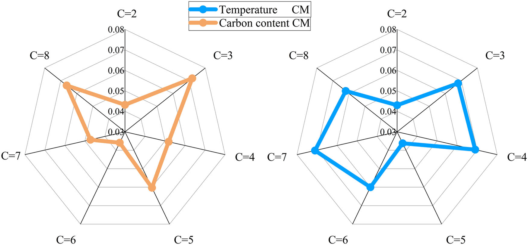
The clustering metrics (CM) defined in this article is a comprehensive clustering metric based on JS distance, taking into account both intra-cluster variance and inter-cluster variance. The existence of λ adjusts the weight of intra-class variance and inter-class variance. In this article, we think that intra-class variance and inter-class variance are equally important, so λ = 0.5.

3.2 A posteriori probability calculation based on JS distance

After the BOF steelmaking process data are clustered, the working conditions of each clustered data are different, and the highly correlated characteristics with the endpoint carbon content and temperature are different under different clustered data. Therefore, determining the affiliation degree of the current sample to be tested for each cluster can indicate the working condition characteristics of the current sample to be tested to a certain extent. Considering that the centroid sample is the average value of each cluster, it can represent the current cluster to a certain extent, so the JS distance is used to measure the JS distance between the current sample to be tested and the centroid of each cluster, and the posterior probability is obtained on this basis. The calculation process is as follows:

Step 1: The JS distance between the sample to be tested x q and the center of mass x k of each class of clusters is calculated according to the JS distance metric criterion, and the likelihood function is obtained according to the following equation:

(8) P ( x q | k ) = JS ( x q , x k ) ∑ k = 1 C JS ( x q , x k ) .

Step 2: Calculate the posterior probability that x q belongs to each category according to the following equations:

(9) P ( k ) = n ( X k ) n ( X ) ,

(10) P ( k | x q ) = P ( x q | k ) P ( k ) ∑ k P ( x q | k ) P ( k ) ,

where P ( k ) is the prior probability of the kth category, and n ( X k ) and n ( X ) denote the number of samples in each category and the number of samples in the entire training set, respectively.

3.3 Calculation of feature weights for different clustered working conditions

After the historical data are spectrally clustered, the variance between the data of different class clusters is large, while the variance of the data within the same class cluster is small. Different clusters have different data characteristics, and the input variables with high correlation with labeled values under different clusters are also different, so it is necessary to measure the correlation between the features of each cluster and the labeled values of the current cluster, to obtain the correlation between the current features and the labeled values of the current cluster, and then finally divide the correlation in each dimension by the sum of correlation in each cluster to obtain the feature weights in the clusters.

The steps for calculating the correlation weights of the features within the class clusters and the labels within the class clusters based on mutual information are as follows:

Step 1: Calculate the mutual information value between the data input features and output values within each class of clusters to obtain the mutual information coefficient between the ith dimension feature f ci of each class of clusters and the output value y c of the current class of clusters. The calculation process is shown in the following equation:

(11) I ( f ci ; y c ) = ∑ ∑ ( f ci , y c ) log p ( f ci , y c ) p ( f ci ) p ( y c ) .

Calculate the intra-class feature weights from the following equation:

(12) w ci = I ( f ci , y c ) ∑ i = 1 d n I ( f ci , y c ) ,

where w k = [ w k 1 , w k 2 , … , w k d n ] , k ⊂ [ 1 , C ] is a vector of feature weights between the features of one of the class clusters and the output, and w ci is the feature weight between the ith dimension feature of the class c cluster and the carbon content or temperature of that class. d n represents the global feature dimension, which is also the feature dimension for each cluster.

Step 2: Calculate the feature weight vector w c for each category of clustered data after clustering, and obtain a vector W = [ w 1 , w 2 , w 3 , … , w c ] with the number of elements equal to the number of clusters, and each element in W represents the feature weight within the cluster under different working conditions.

3.4 Dynamic feature selection process

For the test dataset after feature selection by the FFSDGA, which contains N test data samples of dimension ⅆ n , each of which can be denoted as x q . We compute the mean value of the test dataset in each dimension to get the centroid of this dataset x c , and its center of mass samples in each dimension x cj is computed as follows:

(13) x cj = 1 N test ∑ q = 1 N test x qj , j ∈ [ 1 , d n ] .

Usually, the mean of a dataset is the centroid of the dataset, which represents the average level of a dataset, and the JS distance of the sample to be tested to the centroid represents the degree of its deviation from the centroid; accordingly, we define the volatility of the sample as follows.

Definition 5

The volatility sample is defined as follows:

Calculate the JS distance from each sample to the centroid in the test dataset and arrange them in descending order to form a distance vector D . If the JS distance from the centroid of the current sample is greater than the JS distance from the centroid of the first ∂ ⋅ N test of the samples in the distance vector D , then the current sample is relatively far from the centroid relative to other samples and has volatility.

In the BOF steelmaking process data, some samples to be measured are closer to the centroid, while others are farther away, exhibiting greater volatility. The global feature selection based on the FFSDGA is conducted on the entire dataset and does not account for the dynamic changes arising from sample volatility during the prediction process. Therefore, it is necessary to perform feature selection anew based on the working conditions of the samples to be measured. Accordingly, we define the steps of online dynamic feature selection as follows:

Step 1: When the sample to be tested x q arrives, first calculate the JS distance between the current sample to be tested x q and the centroid x c , and second examine the volatility of the sample according to Definition 5 of volatility above if there is a certain degree of volatility of the sample, the dynamic feature selection mechanism is activated, and if there is no volatility, then it means that the current data is relatively smooth compared with the overall dataset, and can be utilized with the original global features for the regression model prediction.

Step 2: If there is volatility in the current sample to be tested, the dynamic feature selection mechanism needs to be activated, first, a posteriori probability p of the JS distance between the current sample to be tested x q and the centroid sample x k i of each type of cluster is computed to indicate the degree of affiliation of the current sample to be tested to each type of cluster. Its calculation method is shown in the following equation:

(14) P = [ p ( 1 | x q ) , p ( 2 | x q ) , … p ( k | x q ) ] , k ∈ [ 1 , C ] ,

where P is a posteriori probability vector consisting of a posteriori probability that the current sample to be tested belongs to different classes of clusters, and the greater a posteriori probability that the sample to be tested belongs to a certain class, the more its working condition characteristics should conform to which class of working condition characteristics.

For a feature within a cluster after clustering, the larger the weight of the feature within the class means that the feature is more important. Therefore, according to a posteriori probability p that the current sample to be tested belongs to a certain class and the current intra-class feature weight w k , the intra-class feature importance of the current sample to be tested is defined for the kth class. Its calculation method is shown in equation (15)

(15) WCFI k = p ( k | x q ) × w k = [ p ( k | x q ) × w k 1 , p ( k | x q ) × w k 2 , … , p ( k | x q ) × w kdn ] ,

where w k represents the intra-cluster feature weight. The intra-cluster feature weight w k and the posterior probability p ( k | x q ) of the test sample belonging to a certain cluster jointly form the intra-cluster feature importance WCFI k of the current test sample.

Each element of WCFI k represents the intra-cluster feature importance of the current feature in the kth cluster relative to the sample.

For example, WCFI k 1 represents the intra-cluster feature importance of the first global feature in the kth cluster relative to the test sample x q , while WCFI j 1 indicates the intra-cluster feature importance of the first global feature in the jth cluster relative to the test sample x q .

After obtaining the intra-class feature importance WCFI k of the current sample to be tested, we sum the feature importance WCFI k of all clusters to obtain the final feature importance WCFI sum for the sample to be tested. Its calculation method is shown in the following equation:

(16) WCFI sum = WCFI 1 + WCFI 2 + … + WCFI C .

The value of each element at position j in WFKI sum is obtained from the following calculation:

(17) WCFI sum j = WCFI 1 j + WCFI 2 j + … + WCFI cj ,

where WCFI sum j constitutes the vector WCFI sum . Its detailed expression is shown in the following equation:

(18) WCFI sum = [ WCFI sum 1 , WCFI sum 2 , WCFI sum 3 , … , WCFI sum d n ] .

Each element of WCFI sum j represents the feature importance of the current test sample. The larger the value of WCFI sum j , the more important the feature at that position is for the test sample. Therefore, the feature indices corresponding to the top f elements with the largest WCFI sum j values are identified, resulting in the dynamically selected features online. The final feature subset obtained is shown in the following equation:

(19) f DF = [ F 1 , F 2 , F 3 ⋯ F f ] ,

where f DF is the subset of features reselected for volatile samples, obtained by taking the feature indices of the top f maximum elements from WCFI sum . Here, f represents the feature dimension for dynamic feature selection. Finally, we use the dynamically selected feature subset f DF to build the regression model for prediction, obtaining the predicted values y for the volatile samples. When the next volatile sample arrives, the online dynamic mechanism is reactivated to perform dynamic feature selection for it.

4 Dynamic feature selection and JITL soft sensor prediction for endpoint carbon content and temperature

This article employs JITL for regression prediction of endpoint carbon content and temperature in the BOF steelmaking process to validate the effectiveness of the proposed dynamic feature selection algorithm, with JS distance chosen as the similarity measure criterion. The modeling process in this article is shown in Figure 4.

Figure 4

The flowchart of the proposed PPIFW-ODFS soft sensor model.

5 Experiment and result analysis

5.1 Experimental dataset and performance metrics

In the actual BOF steelmaking production process, due to the different dimensions of process data characteristics, it is necessary to standardize the original data to eliminate the influence of dimensions between data. The original data set is Data = { ( x i , y ) ⊂ R d + 1 ; i = 1 , 2 … d } , where x i is the input characteristics of the BOF steelmaking process data, such as the amount of oxygen blowing, the total of transferred, and so on. y is the label value of the endpoint carbon content or temperature, and d is the dimension of the input data.

Accurate prediction of carbon content and temperature in the molten pool is the key to controlling the endpoint of BOF steelmaking. The experimental data originate from the actual BOF steelmaking production process of a steel plant. These data are sourced from the production process of a 120-ton BOF, where the oxygen-blowing duration is approximately 18 min. The entire production cycle for a single heat, which includes stages such as raw material charging, typically lasts around 30 min.

The input variables include the location of oxygen lance, oxygen blowing time, manganese content in molten iron, and so on, and the data with 30-dimensional characteristics are selected for the experiments by eliminating the anomalies with the negative and all-zero ranks, and the data of the endpoint carbon content and temperature are taken as the corresponding output variables with the data variables are shown in Table 1.

Table 1

Input characteristics

Target variables	Input variables
Carbon content	No. 1: Charged amount of molten iron	No. 2: Total of transferred
	No. 3: Temperature of iron	No. 4: Carbon content in molten iron
	No. 5: Silicon content in molten iron	No. 6: Manganese content in molten iron
	No. 7: Sulfur content in molten iron	No. 8: Phosphorus content in molten iron
	No. 9: Arsenic content in molten iron	No. 10: Time to mix iron
	No. 11: End of iron mixing to oxygen opening time	No. 12: Average location of oxygen lance
	No. 13: Average oxygen pressure	No. l4: Location of oxygen lance 1
	No. 15: Location of oxygen lance 2	No. 16: Location of oxygen lance 3
	No. 17: Location of oxygen lance 4	No. 18: Location of oxygen lance 5
	No. 19: Location of oxygen lance 6	No. 20: Location of oxygen lance 22
	No. 21: Location of oxygen lance 23	No. 22: Location of oxygen lance 24
	No. 23: Oxygen pressure 1	No. 24: Oxygen pressure 2
	No. 25: Oxygen blowing time	No. 26: Oxygen blowing amount
	No. 27: Oxygen pressure 3	No. 28: Amount of dolomite added
	No. 29: Amount of lime added	No. 30: The time from tapping to starting to mix iron
Temperature	No. 1: Charged amount of molten iron	No. 2: Total transferred
	No. 3: Carbon content in molten iron	No. 4 Silicon content in molten iron
	No. 5: Manganese content in molten iron	No. 6: Sulfur content in molten iron
	No. 7: Phosphorus content in molten iron	No. 8: Time to mix iron
	No. 9: The time from tapping to starting to mix iron	No. 10: Amount of lime added
	No. 11: Amount of dolomite added	No. 12: Oxygen blowing time
	No. 13: Oxygen blowing amount	No. 14: Average location of oxygen lance
	No. 15: Average oxygen pressure	No. 16: Location of oxygen lance 1
	No. 17: Location of oxygen lance 2	No. 18: Location of oxygen lance 3
	No. 19: Location of oxygen lance 4	No. 20: Location of oxygen lance 5
	No. 21: Location of oxygen lance 6	No. 22: Location of oxygen lance 7
	No. 23: Location of oxygen lance 8	No. 24: Location of oxygen lance 9
	No. 25: Location of oxygen lance 10	No. 26: Location of oxygen lance 11
	No. 27: Location of oxygen lance 12	No. 28: Location of oxygen lance 13
	No. 29: Location of oxygen lance 14	No. 30: Location of oxygen lance 15

During the experiment, 1,000 sample normal operation state data points were collected. Among them, 800 data points were used for the training set, 100 data points were used for the validation set, and 100 data points were used for the test set. To evaluate the prediction performance of various soft sensor models, this article adopts the PA, root mean square error (RMSE), and mean absolute percentage error (MAPE) as the evaluation metrics. Higher PA indicates higher PA and smaller values of RMSE and MAPE indicate better prediction performance. These indicators are calculated as follows:

(20) PE i = 1 , | y test , i − y pre , i | ≤ Th 0 , | y test , i − y pre , i | > Th ,

(21) PA = ∑ i = 1 N test PE i N test ,

(22) RMSE = 1 N test ∑ i = 1 N test ( y test , i − y pre , i ) 2 ,

(23) MAPE = 1 N test ∑ i = 1 N test y test , i − y pre , i y test , i ,

where N test denotes the number of test samples i ⊂ ( 1 , N test ) ; y pre and y test denote predicted and actual values; PA denotes the prediction accuracy within the margin of error; and PE i means that the prediction is hit when the error is within the error range (Th). The PA error threshold for carbon content is Th = 0.02%, while for temperature, it is Th = ±10°C.

Due to the extensive use of algorithm abbreviations in the subsequent ablation and comparative experiments, we have provided a list of abbreviations to clarify the meanings of all abbreviations used in the article, thereby enhancing its readability. The list of abbreviations is shown in Table 2.

Table 2

Abbreviation definitions

Abbreviations	Full form
BOF	Basic oxygen furnace
PPIFW-ODFS	Posterior probability and intra-cluster feature weight online dynamic feature selection
JS	Jensen–Shannon
MAE	Mean absolute error
JITL	Just-in-time learning
PA	Prediction accuracy
RMSE	Root mean square error
MAPE	Mean absolute percentage error
CM	Clustering metrics
FFSDGA	Fixed feature space dimensions genetic algorithm
GA	Genetic algorithm
GWO	Grey wolf optimization algorithm
ACO	Ant colony optimization algorithm
AMPGA	Adaptive mutation probability genetic algorithm
WFS	Without feature selection
MB	Markov blanket feature selection algorithm
MDA-SEL	Multi-cluster dynamic adaptive selection ensemble learning
SWLSPPDR	Supervised weighted local structure preserving projection dimensionality reduction
vMF-WSAE	vMF-WSAE dynamic deep learning

5.2 Visualization of global feature data

In this experiment, we utilize the global feature data selected by the FFSDGA. These data are normalized using max–min normalization, ensuring that each eigenvalue falls between 0 and 1.

Thereafter, we calculate the mean value of the samples across each dimension in the global feature data to obtain the centroid sample. Subsequently, we measure the JS distance between the dataset samples and the centroid sample to illustrate the fluctuation of the samples. The data visualization is presented in Figure 5.

Figure 5

Visualization of global feature data volatility.

5.3 Determining the optimal number of clusters c

The CM index defines the evaluation function for data clustering in BOF steelmaking. By varying the number of clusters, we obtain the values of intra-class variance and Inter-class variance, standardized to a common scale, for different cluster numbers, and calculate the corresponding CM values to determine the optimal number of clusters. In the offline stage, we set the number of clusters C from 2 to 8 and conducted experiments on two datasets: temperature and carbon content. By comparing the results, we determine the reasonable number of clusters for historical furnace samples in predicting the endpoint of carbon content and temperature, which are 6 and 5, respectively. The CM values for different numbers of clusters for carbon content and temperature are shown in Figure 6.

$Figure 6 CM {\rm{CM}} values for different numbers of clusters C C .$

Figure 6

CM values for different numbers of clusters C .

5.4 Determination of the number of preset feature selections d n for FFSDGAs

The fixed feature space dimensions feature selection algorithm requires setting the number of features in advance before starting the algorithm. Since the MAE defines the fitness function of feature selection, the MAE of the optimal individual is obtained under different numbers of feature selections to determine the optimal number of features. At the offline stage, the number of feature selections d n is varied from 5 to 12. Experiments are conducted on two datasets, namely, temperature and carbon content. Each experiment with the preset number of features is repeated independently 10 times to obtain the MAE corresponding to the optimal individual and find the optimal number of features. Experimental results reveal that the lowest MAE individual is achieved when the number of preset features is 9. The optimal fitness for the different number of preset features for carbon content and temperature is shown in Figure 7.

$Figure 7 MAE corresponding to different global feature selection numbers d n {d}_{n} .$

Figure 7

MAE corresponding to different global feature selection numbers d n .

5.5 Determination of key parameters of the online section

In the subsequent experiments, the modeling process of the PPIFW-ODFS method involves the following key parameters. First, the determination of the number f of feature selections for volatile samples. Second, the determination of the distance threshold for volatile samples ∂ . Third, the determination of the number S of subsets of similar samples.

Each optimal parameter is selected as follows: in the experimental simulation, first, the number of low-dimensional feature selection features is looped with a step size of 1, conducting the first level of loop traversal in the interval [2,8]. Second, the threshold of the JS distance from the sample to be tested to the center of the test set is looped with a step size of 0.01, performing the second level of loop traversal in the interval [0.8,1]. Then, under the precondition of the first two levels of loop traversal, the number of similar samples is looped with 1 as the step size, conducting a third loop traversal in the interval [1,100]. Since the accuracy of different parameters may be repetitive, the evaluation index is chosen to realize all possible traversal loops of the three parameters through three layers of loops, and the best parameters are obtained by iterating. The optimal parameters are shown in Table 3.

Table 3

Experimental parameter settings

Optimal parameter	f	∂	S	RMSE
Carbon content	4	0.83	74	0.01381
Temperature	3	0.92	55	6.55232

5.5.1 Determination of the dynamic feature selection parameter f

The key to this section of the experiment lies in the determination of the number of feature selections f of the volatility samples, and a reasonable number of feature selections of the volatility samples can not only provide key feature information but also avoid the interference of redundant information. After the above cycle of experiments to verify, in the case of other parameters that are optimal, carbon content volatility samples of the number of features of 4, and the number of temperature feature selection of 3 can get the optimal prediction results. We adopt the control variable method RMSE as the evaluation index to visualize the effect of the number of dynamically selected features on the results under the condition of other parameters being optimal, as shown in Figure 8.

Figure 8

RMSE corresponding to different dynamic feature selection f.

5.5.2 Determination of dynamic feature selection volatility threshold ∂

In dynamic feature selection, the identification of volatile samples is crucial, and an appropriate distance threshold can aid in locating volatile samples within the test set, thereby enabling online dynamic feature selection to enhance the model’s predictive performance. We calculate the JS distance from each test sample x q to the test set centroid x c to obtain the distance vector D . If the distance from the current sample x q to the centroid x c exceeds the distances of N test ⋅ ∂ test samples to the test set centroid x c , it indicates that this sample is relatively far from the test set centroid, suggesting a certain level of volatility, where N test is the number of samples in the test set.

Therefore, this experiment utilized a step size of 0.01 and conducted a search within the interval of [0.8,1]. It was verified through the aforementioned cyclic experiments that optimal prediction results can be achieved when the carbon content is at a distance threshold of ∂ of 0.83, and the temperature dataset is at a distance threshold of ∂ of 0.92. We used the control variable method with RMSE as the evaluation index to visualize the effect of the volatility threshold on the results under the condition that the other parameters are tuned to the optimum, as shown in Figure 9.

Figure 9

RMSE corresponding to different volatility thresholds ∂.

5.5.3 Determination of the number of subsets of similar samples S

In JITL, the selection of the number of similar samples S has a significant impact on the results. In this experiment, the step size is set to 1, and the search is traversed cyclically between [1,100]. It is experimentally verified that the optimal prediction results can be obtained when the number of similarity samples of carbon content is 74 and the number of similarity samples of temperature is 55. We use the control variable method with RMSE as the evaluation index to visualize the effect of the number of similar samples on the results under the condition of other parameters being optimal, as shown in Figure 10.

Figure 10

RMSE corresponding to different numbers of similar sample subsets S.

5.6 Comparison of FFSDGA with other feature selection algorithms

To prove that the FFSDGA in this article obtains more stable industrial features of BOF steelmaking by the method of predefined features, this section demonstrates the advantages of this article’s algorithm in selecting global feature stability by comparing the literature with the GA [24], the Grey wolf optimization (GWO) algorithm [25], the ant colony optimization (ACO) algorithm [26], and adaptive mutation probability genetic algorithm (AMPGA) [27]. Ten independent experiments are conducted on the carbon content and temperature datasets, respectively, to record the number of selected features and the optimal fitness values, as illustrated in Figures 11 and 12.

Figure 11

Comparison of adaptation with other feature selection methods.

Figure 12

Stability comparison with other feature selection methods.

From Figures 11 and 12, it can be seen that the FFSDGA with the number of preset features proposed in this article is slightly better than other optimization algorithms in terms of the ability to find the optimal, and from the box plot, it can be seen that the stability of this article’s GA feature selection choosing out of global feature selection is much better than other algorithms, and obtains a more stable industrial production features, which proves the validity of the preset features.

5.7 Experiments on longitudinal ablation of dynamic feature selection algorithms and cross-sectional comparison with other feature selection algorithms

In this section, ablation experiments are conducted to validate the effectiveness of the proposed algorithms, specifically the without feature selection (WFS) algorithm, the offline FFSDGA, and the PPIFW-ODFS algorithm.

The effectiveness of the proposed method at the feature selection level is further highlighted by a horizontal comparison of various feature selection algorithms, including the Markov blanket (MB) feature selection algorithm [28], GWO algorithm, ACO algorithm, and AMPGA algorithm. Additionally, this section provides a horizontal comparison of other methods applied to the BOF steelmaking process, such as multi-cluster dynamic adaptive selection ensemble learning (MDA-SEL) [29], supervised weighted local structure preserving projection dimensionality reduction (SWLSPPDR) [30], and vMF-WSAE dynamic deep learning [31]. The significance of dynamic feature selection in handling real-variable volatility data is thereby validated. The parameters of the compared methods have been optimized, and the prediction results are presented in Figures 13 and 14. Relevant performance indicators are summarized in Table 4.

Figure 13

Comparison of various carbon content prediction models. (a) WFS. (b) FFSDGA. (c) MB. (d) GWO. (e) ACO. (f) AMPGA. (g) MDA-SEL. (h) SWLSPPDR. (i) vMF-WSAE. (j) PPIF-ODFS.

Figure 14

Comparison of various temperature prediction models. (a) WFS. (b) FFSDGA. (c) MB. (d) GWO. (e) ACO. (f) AMPGA. (g) MDA-SEL. (h) SWLSPPDR. (i) vMF-WSAE. (j) PPIF-ODFS.

Table 4

Analysis of various model evaluation metrics

Indicators	Th	WFS	FFSDGA	MB [28]	GWO [25]	ACO [26]
Carbon content PA	0.02%	76%	80%	78%	79%	79%
Carbon content RMSE	—	0.0175	0.0154	0.0162	0.0150	0.016
Carbon content MAPE	—	0.148	0.124	0.148	0.159	0.144
Temperature PA	± 10 ° C	74%	85%	78%	80%	81%
Temperature RMSE	—	8.943	7.101	7.874	7.910	7.940
Temperature MAPE	—	0.0045	0.0035	0.0041	0.0041	0.0040

Indicators	Th	AMPGA [27]	MDA-SEL [29]	SWLSPPDR [30]	vMF-WSAE [31]	PPIFW-ODFS
Carbon content PA	0.02%	81%	73%	71%	78%	86%
Carbon content RMSE	—	0.0153	0.0168	0.0178	0.0158	0.0138
Carbon content MAPE	—	0.1472	0.1572	0.1838	0.1456	0.109
Temperature PA	± 10 ° C	83%	74%	75%	80%	88%
Temperature RMSE	—	7.390	8.401	8.6455	7.7489	6.5523
Temperature MAPE	—	0.0038	0.0042	0.0043	0.0039	0.0033

The accuracy of predicting carbon content and temperature directly using the WFS is depicted in Figures 13(a) and 14(a), with values of 76.00 and 74.00%, respectively. In contrast, the accuracy of predicting carbon content and temperature using the global features selected by the FFSDGA is shown in Figures 13(b) and 14(b), which are 80.00 and 85.00%. This demonstrates that the global features thereby improve the model’s PA.

However, this algorithm does not significantly enhance the accuracy of carbon content compared to temperature. As discussed in Section 5.2, this limitation arises because the carbon content dataset exhibits greater sample fluctuation than the temperature dataset, and the FFSDGA cannot dynamically select features. To address the feature offset problem caused by data volatility, the PPIFW-ODFS proposed in this article, as shown in Figures 13(j) and 14(j), achieves prediction accuracies of 86.00% for carbon content and 88.00% for temperature. This indicates that the re-selected features for volatile samples are better suited to the current operating conditions. The longitudinal ablation comparison results of these three approaches demonstrate that the PPIFW-ODFS algorithm effectively addresses data redundancy and the time-varying nature of features in the BOF steelmaking process.

The accuracy of predicting carbon content and temperature using the MB feature selection algorithm is 78.00% for both carbon content and temperature, as shown in Figures 13(c) and 14(c). In contrast, the PPIFW-ODFS method proposed in this article achieves accuracies of 86.00% for carbon content and 88.00% for temperature, as shown in Figures 13(j) and 14(j). This difference can be attributed to the fact that, while the MB algorithm considers feature redundancy and the correlation between features and the target variable, its performance is constrained by the complexity of the BOF steelmaking process data when relying solely on statistical measures for feature selection. Furthermore, this algorithm does not account for dynamic changes in features during the prediction process.

The accuracy of carbon content and temperature prediction using the GWO algorithm is 79.00 and 80.00%, respectively, as shown in Figures 13(d) and 14(d). The ACO algorithm achieves accuracies of 81.00% for carbon content and 81.00% for temperature, as shown in Figures 13(e) and 14(e). The AMPGA algorithm results in accuracies of 81.00% for carbon content and 83.00% for temperature, as shown in Figures 13(f) and 14(f). In contrast, the PPIFW-ODFS method proposed in this article achieves accuracies of 86.00% for carbon content and 88.00% for temperature, as shown in Figures 13(j) and 14(j). The comparison of these three wrapper-based feature selection algorithms indicates that the PPIFW-ODFS method not only effectively selects high-quality global features using a predefined number of features but also addresses data fluctuation and feature drift in the BOF steelmaking process through its dynamic approach. In contrast, the three compared methods fail to account for feature drift during the global feature selection process and lack a predefined number of features, resulting in inferior prediction performance.

Furthermore, from the perspective of predicting endpoint carbon content and temperature in BOF steelmaking, this article compares three other soft sensor methods: SWLSPPDR, as shown in Figures 13(g) and 14(g), SWLSPPDR as shown in Figures 13(h) and 14(h), and vMF-WSAE as shown in Figures 13(i) and 14(i). The MDA-SEL method achieves prediction accuracies of 73% for carbon content and 74% for temperature. The SWLSPPDR method results in accuracies of 71% for carbon content and 75% for temperature. The vMF-WSAE method attains accuracies of 78% for carbon content and 80% for temperature. Although the MDA-SEL method enhances the model’s capability to extract complex data from the BOF steelmaking process through a multi-cluster ensemble approach, it suffers from suboptimal clustering results due to the absence of feature selection and its failure to account for dynamic changes in features during the prediction process, adversely affecting the final recognition rate of the ensemble learning. The SWLSPPDR method relies excessively on sparse representations and exhibits limited adaptability to fluctuating data. Lastly, the vMF-WSAE dynamic deep learning method, while fine-tuning deep learning with the vMF distribution, only addresses sample-level adjustments and does not account for dynamic feature changes, resulting in lower recognition rates compared to the method proposed in this article.

5.8 Randomized feature selection experiments for online volatility samples

In order to prove that the online partial dynamic features selected for the fluctuation samples are the optimal features for the current working conditions, this article conducts experiments on randomly generating features for the fluctuation samples, using random seeds to randomly generate random features for the fluctuation samples to participate in the prediction and comparing them with the features selected by the dynamic feature selection algorithm proposed in this article. Five sets of experiments were repeated independently with the same optimal parameters to demonstrate the effectiveness of the proposed method. The prediction results of carbon content and temperature are shown in Figures 15 and 16. The relevant performance indicators are shown in Table 5.

Figure 15

Plot of carbon content prediction results. (a) The first random feature generation for volatile samples. (b) The second random feature generation for volatile samples. (c) The third random feature generation for volatile samples. (d) The fourth random feature generation for volatile samples. (e) The fifth random feature generation for volatile samples. (f) The method in this paper.

Figure 16

Plot of temperature prediction results. (a) The first random feature generation for volatile samples. (b) The second random feature generation for volatile samples. (c) The third random feature generation for volatile samples. (d) The fourth random feature generation for volatile samples. (e) The fifth random feature generation for volatile samples. (f) The method in this paper.

Table 5

Comparative analysis of randomly generated feature experiment and the proposed method

Indicators	Th	First	Second	Third	Fourth	Fifth	PPIFW-ODFS
Carbon content PA	0.02%	82%	79%	80%	82%	80%	86%
Carbon content RMSE	—	0.0146	0.0156	0.0154	0.0154	0.0155	0.0138
Carbon content MAPE	—	0.126	0.135	0.135	0.133	0.134	0.109
Temperature PA	± 10 ° C	85%	85%	86%	85%	84%	88%
Temperature RMSE	—	7.3412	7.0066	7.00	7.10	7.36	6.5523
Temperature MAPE	—	0.0036	0.0035	0.0035	0. 0035	0.0036	0.0033

The experimental results show that the PA, RMSE, and MAPE of our proposed dynamic feature selection method are better than the online random feature selection method. The experiments prove that the dynamic feature selection algorithm proposed in this article can overcome the volatility of the data of the BOF steelmaking process, realize the dynamic feature selection of the fluctuating samples, and improve the PA.

6 Conclusion

In this article, due to the complexity of the BOF steelmaking process, the addition of sensors has resulted in high-dimensional data, redundancy among features, variability in data characteristics due to raw material quality differences, and errors introduced by manual operations. Consequently, global feature selection modeling is inadequate for the current working conditions. An online dynamic feature selection method based on posterior probabilities and intra-cluster feature weights is proposed to address these challenges.

In the offline phase, a FFSDGA for feature selection is proposed. This approach reduces the solution space of the GA by presetting the number of features to be selected before the feature selection process, thereby achieving more stable industrial features.

In the online phase, to address the limitation that global feature selection modeling with an FFSDGA cannot adapt to dynamic feature changes, historical samples are clustered into groups with small intra-class variance and large inter-class variance. By leveraging the posterior probability that a test sample belongs to a specific cluster, along with the feature weights within each cluster, features are dynamically selected for fluctuating samples to accommodate data variability.

The modeling simulation of BOF steelmaking process data verifies the effectiveness of this method for predicting carbon content and temperature at the endpoint of the BOF steelmaking process. Compared with traditional feature selection methods, this approach selects features that align with the current working conditions of the test samples for modeling, thereby overcoming the volatility of the BOF steelmaking process data and holding certain value in practical soft sensor applications.

Acknowledgements

The authors are grateful to the National Natural Science Foundation of China (No. 62263016), the Applied Basic Research Foundation of Yunnan Province (No. 202401AT070375), the project ‘Yunnan Xingdian Talents Support Plan,’ and the ‘Yunnan Provincial University Service Key Industry Science and Technology Program (FWCY-QYCT2024003)’ for their financial support of this research.

Funding information: This work was supported by the National Natural Science Foundation of China (No. 62263016); the Applied Basic Research Foundation of Yunnan Province (No. 202401AT070375); supported by the project “Yunnan Xingdian Talents Support Plan”; and “Yunnan Provincial University Service Key Industry Science and Technology Program (FWCY-QYCT2024003)”.
Author contributions: Haodong Wang: conceptualization, methodology, software, validation, writing – original draft, writing – review editing, visualization. Hui Liu: corresponding author, conceptualization, methodology, supervision, project administration, funding acquisition. FuGang Chen: data curation, formal analysis, investigation. Heng Li: investigation. XiaoJun Xue: investigation.
Conflict of interest: The authors state no conflict of interest.
Data availability statement: The data cannot be made publicly available upon publication because they contain commercially sensitive information. The data that support the findings of this study are available upon reasonable request from the authors.

References

[1] Holappa, L. Historical overview on the development of converter steelmaking from Bessemer to modern practices and future outlook. Mineral Processing and Extractive Metallurgy, Vol. 128, No. 1–2, 2019, pp. 3–16.10.1080/25726641.2018.1539538Suche in Google Scholar

[2] Hooey, L., A. Tobiesen, J. Johns, and S. Santos. Techno-economic study of an integrated steelworks equipped with oxygen blast furnace and CO2 capture. Energy Procedia, Vol. 37, 2013, pp. 7139–7151.10.1016/j.egypro.2013.06.651Suche in Google Scholar

[3] Han, M., Y. Li, and Z. Cao. Hybrid intelligent control of BOF oxygen volume and coolant addition. Neurocomputing, Vol. 123, 2014, pp. 415–423.10.1016/j.neucom.2013.08.003Suche in Google Scholar

[4] Chen, Y., X. T. Liang, J. H. Zeng, J. Chen, and R. D. Liu. Numerical simulation and optimization practice of oxygen lance for converter steelmaking. Advanced Materials Research, Vol. 402, 2012, pp. 156–159.10.4028/www.scientific.net/AMR.402.156Suche in Google Scholar

[5] Feng, S. C., Y. H. Wang, and R. F. Ding. Application status of end-point control technologies in converter steelmaking. Metallurgical Industry Automation, Vol. 40, No. 2, 2016, pp. 1–6.Suche in Google Scholar

[6] Xu, G., H. B. Lei, J. H. Li, Y. P. Ye, and J. Xue. End-point control techniques for converter steel-making. Steelmaking, Vol. 27, No. 1, 2011, pp. 66–70.Suche in Google Scholar

[7] Zhang, C., Y. Zhang, and Y. Han. Industrial cyber-physical system driven intelligent prediction model for converter end carbon content in steelmaking plants. Journal of Industrial Information Integration, Vol. 28, 2022, id. 100356.10.1016/j.jii.2022.100356Suche in Google Scholar

[8] Hu, Z., L. Liu, and P. He. Application of gas analysis in converter dynamic control. Journal of Iron and Steel Research, Vol. 14, No. 3, 2002, pp. 68–72.Suche in Google Scholar

[9] Tao, J., Z. G. Chen, W. D. Qian, and X. Wang. Intelligent control method for BOF steelmaking process. Proceedings of the World Engineers’ Convention 2004, Vol A, Network Engineering and Information Society, 2004, pp. 345–350.Suche in Google Scholar

[10] Ao, X. Converter steelmaking endpoint control technology application analysis. Metallurgy and Materials, Vol. 39, No. 5, 2019, pp. 110–112.Suche in Google Scholar

[11] Wen, H. Y. and M. C. Zhou. Current status and application of converter end-point control technology. Modern Industrial Economy and Informationization, Vol. 9, No. 2, 2019, pp. 79–81.Suche in Google Scholar

[12] Xie, S. M., T. Y. Chai, and J. Tao. A kind of new method for LD dynamic endpoint prediction. Acta Automatica Sinica, Vol. 1, 2001, pp. 136–139.Suche in Google Scholar

[13] Liu, C., Y. Zhang, and X. Zhang. A soft measure algorithm for BOF steelmaking process. Control Engineering of China, Vol. 23, No. 9, 2016, pp. 1312–131.Suche in Google Scholar

[14] Fan, M., Z. Ge, and Z. Song. Adaptive Gaussian mixture model-based relevant sample selection for JITL soft sensor development. Industrial & Engineering Chemistry Research, Vol. 53, No. 51, 2014, pp. 19979–19986.10.1021/ie5029864Suche in Google Scholar

[15] Yuan, X., B. Huang, Y. Wang, C. Yang, and W. Gui. Deep learning-based feature representation and its application for soft sensor modeling with variable-wise weighted SAE. IEEE Transactions on Industrial Informatics, Vol. 14, No. 7, 2018, pp. 3235–3243.10.1109/TII.2018.2809730Suche in Google Scholar

[16] Liu, Y., D. Huang, B. Liu, Q. Feng, and B. Cai. Adaptive ranking based ensemble learning of Gaussian process regression models for quality-related variable prediction in process industries. Applied Soft Computing, Vol. 101, 2021, id. 107060.10.1016/j.asoc.2020.107060Suche in Google Scholar

[17] Hui, K. H., C. S. Ooi, M. H. Lim, M. S. Leong, and S. M. Al-Obaidi. An improved wrapper-based feature selection method for machinery fault diagnosis. PloS One, Vol. 12, No. 12, 2017, id. e0189143.10.1371/journal.pone.0189143Suche in Google Scholar PubMed PubMed Central

[18] Bommert, A., X. Sun, B. Bischl, J. Rahnenführer, and M. Lang. Benchmark for filter methods for feature selection in high-dimensional classification data. Computational Statistics & Data Analysis, Vol. 143, 2020, id. 106839.10.1016/j.csda.2019.106839Suche in Google Scholar

[19] Maleki, N., Y. Zeinali, and S. T. A. Niaki. A k-NN method for lung cancer prognosis with the use of a genetic algorithm for feature selection. Expert Systems with Applications, Vol. 164, 2021, id. 113981.10.1016/j.eswa.2020.113981Suche in Google Scholar

[20] Asghari, S., H. Nematzadeh, E. Akbari, and H. Motameni. Mutual information-based filter hybrid feature selection method for medical datasets using feature clustering. Multimedia Tools and Applications, Vol. 82, No. 27, 2023, pp. 42617–42639.10.1007/s11042-023-15143-0Suche in Google Scholar

[21] Chamlal, H., T. Ouaderhman, and F. Aaboub. A graph based preordonnances theoretic supervised feature selection in high dimensional data. Knowledge-Based Systems, Vol. 257, 2022, id. 109899.10.1016/j.knosys.2022.109899Suche in Google Scholar

[22] Hermo, J., V. Bolón-Canedo, and S. Ladra. Fed-mRMR: A lossless federated feature selection method. Information Sciences, Vol. 669, 2024, id. 120609.10.1016/j.ins.2024.120609Suche in Google Scholar

[23] Nielsen, F. On the Jensen–Shannon symmetrization of distances relying on abstract means. Entropy, Vol. 21, No. 5, 2019, id. 485.10.3390/e21050485Suche in Google Scholar PubMed PubMed Central

[24] Xue, Y., H. Zhu, J. Liang, and A. Słowik. Adaptive crossover operator based multi-objective binary genetic algorithm for feature selection in classification. Knowledge-Based Systems, Vol. 227, 2021, id. 107218.10.1016/j.knosys.2021.107218Suche in Google Scholar

[25] Al-Tashi, Q., S. J. Abdul Kadir, H. M. Rais, S. Mirjalili, and H. Alhussian. Binary optimization using hybrid grey wolf optimization for feature selection. IEEE Access, Vol. 7, 2019, pp. 39496–39508.10.1109/ACCESS.2019.2906757Suche in Google Scholar

[26] Peng, H., C. Ying, S. Tan, B. Hu, and Z. Sun. An improved feature selection algorithm based on ant colony optimization. IEEE Access, Vol. 6, 2018, pp. 69203–69209.10.1109/ACCESS.2018.2879583Suche in Google Scholar

[27] Liu, H., P. Zeng, Q. Wu, and F. Chen. Feature selection for converter steelmaking process data based on an improved genetic algorithm. Journal of Instruments and Instrumentation, Vol. 40, No. 12, 2019, pp. 185–195.Suche in Google Scholar

[28] Hua, Z., J. Zhou, Y. Hua, and W. Zhang. Strong approximate Markov blanket and its application on filter-based feature selection. Applied Soft Computing, Vol. 87, 2020, id. 105957.10.1016/j.asoc.2019.105957Suche in Google Scholar

[29] Shao, B., H. Liu, and F. Chen. Soft sensor method for endpoint carbon content and temperature of BOF based on multi-cluster dynamic adaptive selection ensemble learning. High Temperature Materials and Processes, Vol. 42, No. 1, 2023, id. 20220287.10.1515/htmp-2022-0287Suche in Google Scholar

[30] Su, Y., H. Liu, F. Chen, J. Liu, H. Li, and X. Xue. BOF steelmaking endpoint carbon content and temperature soft sensor model based on supervised weighted local structure preserving projection. High Temperature Materials and Processes, Vol. 43, No. 1, 2024, id. 20240030.10.1515/htmp-2024-0030Suche in Google Scholar

[31] Yang, L., H. Liu, and F. Chen. Soft sensor method of multimode BOF steelmaking endpoint carbon content and temperature based on vMF-WSAE dynamic deep learning. High Temperature Materials and Processes, Vol. 42, No. 1, 2023, id. 20220270.10.1515/htmp-2022-0270Suche in Google Scholar

Received: 2024-07-08

Revised: 2024-11-24

Accepted: 2024-11-25

Published Online: 2025-01-16

This work is licensed under the Creative Commons Attribution 4.0 International License.

Artikel in diesem Heft

https://doi.org/10.1515/htmp-2024-0067

Schlagwörter für diesen Artikel

BOF steelmaking; soft sensor; online dynamic feature selection algorithm; genetic algorithm

Creative Commons

BY 4.0