Prediction model of BOF end-point P and O contents based on PCA–GA–BP neural network
-
Zhao Liu
 and
Pengbo Liu
and
Pengbo Liu

Abstract
Low-carbon, green and intelligent production is urgently needed in China’s iron and steel industry. Accurate prediction of liquid steel composition at the end of basic oxygen furnace (BOF) plays an important role in promoting high-quality, high-efficiency and stable production in steelmaking process. A prediction model based on the principal component analysis (PCA) – genetic algorithm (GA) – back propagation (BP) neural network is proposed for BOF end-point P and O contents of liquid steel. PCA is used to eliminate the correlation between the factors, and the obtained principal components are seen as input parameters of the BP neural network; then, GA is employed to optimize the initialized weights and thresholds of the BP neural network. The flux composition and bottom blowing are considered in the input variables. The results indicate that the prediction accuracy of the single output model is higher than that of the dual output model. The root-mean-square error of P content between predicted and actual values is 0.0015%, and that of O content is 0.0049%. Therefore, the model can provide a good reference for BOF end-point control.
1 Introduction
Basic oxygen furnace (BOF) process is the most important steelmaking method in China. Accurately predicting the liquid steel composition at the end-point of the BOF is of great importance to achieve emission reduction, consumption reduction, green and efficient production. The phosphorus and oxygen contents of the liquid steel are a very important factor for end-point control of BOF, which has a significant impact on product quality and plant economics. Since the process after BOF has no dephosphorization function, phosphorus must be removed to the desired level in the BOF process. Phosphorus concentrations below 0.01% may generally be required to avoid embrittlement [1]. Many steel plants have adopted high-efficiency dephosphorization technology in BOF due to the increasing demand for low and ultra-low phosphorus steels [2,3,4]. In addition, the oxygen content of the liquid steel at the end-point has a significant influence on the alloy consumption, desulfurization and inclusion removal of the subsequent processes. In summary, if the content of phosphorus and oxygen at the end-point of BOF can be controlled more accurately, the quality of liquid steel will be further improved.
The physical and chemical reactions with a high temperature in BOF and the fluctuation of raw materials composition make it still a challenge to accurately predict the composition of the liquid steel at the end-point. At the same time, there exists a complex non-linear relationship between the variables affecting the liquid steel composition at the end of BOF. Therefore, linear regression models and thermodynamic-based mathematical models are difficult to obtain better prediction results. Artificial neural network (ANN) has the capability of self-study, self-adaptation, and self-organization, which can simulate complicated functions. At present, some prediction methods based on neural networks or neural network combined algorithms have been widely used in BOF end-point control [5]. For example, Wang et al. [6] applied weighted K-means clustering and a group method of data handling (GMDH), combined with a separate neural network for each cluster. Using this method, they reported a phosphorus prediction accuracy of 88.40%, with an error tolerance of ±0.004%. He and Zhang [7] proposed a model based on principal component analysis (PCA) and backpropagation (BP) neural network for predicting the BOF end-point phosphorus content. They achieved hit rates of 92.06 and 82.54% within error bond ±0.004 and ±0.003%, which is higher than those of multiple linear regression and ordinary BP neural networks. Bae et al. [8] examined the prediction accuracy of seven standard machine learning algorithms using a large production data set with the aim of predicting the BOF end-point. The results showed that ANN has better predictive performance than other algorithms and gets an 89% hit rate with an error of ±0.003%. Zhou et al. [9] established a prediction model of end-point phosphorus content for BOF based on a monotone-constrained BP neural network. The model using the constraint condition achieved a prediction accuracy of 74% with an error of ±0.003%. Zhou et al. [10] selected seven input variables according to the grey correlation analysis as the input of the BP neural network. The authors claimed the hit rate to be 83.33% when the range of phosphorus error is ±0.004%. It can be seen that the ANN with high prediction accuracy is widely used for end-point phosphorus content prediction. Moreover, there are many prediction models of liquid steel temperature, carbon content and manganese content based on intelligent algorithms in previous studies [11,12,13,14,15,16].
However, few works are investigating the prediction of the oxygen content of liquid steel. In addition, researchers usually considered the weight of the flux in the input variables and ignored the chemical composition of the flux. To enhance the accuracy of predicting the BOF end-point phosphorus and oxygen contents of liquid steel, a hybrid model based on PCA, genetic algorithm (GA), and BP neural network is proposed. PCA is used to reduce the dimensionality of the input variables and eliminate the collinearity among the variables, rather than deleting variables with a high coincidence degree [17]. GA is employed to optimize the initialized weights and thresholds of the BP neural network to overcome BP’s disadvantage of being easily stuck in a local minimum. Therefore, the PCA–GA–BP neural network has the ability to search globally and approach any non-linear functions with any precision.
2 Model establishment
2.1 Input and output parameters
The schematic diagram of BOF steelmaking is shown in Figure 1. During the process, oxygen is used to react with the elements in the liquid steel, and the components in the flux react with the oxidation products to obtain suitable slag, which contains necessary basicity, MgO content and FeO content. At the same time, the bottom blowing process can enhance the stirring of the metal pool and reduce the equilibrium oxygen content in liquid steel.

Schematic of BOF steelmaking.
According to the metallurgical mechanism and production practice, end-point liquid steel composition is mainly determined by the factors listed in Table 1. It should be noted that the fluctuation of flux composition will affect the stability of the steelmaking process, so the chemical composition of the flux must be considered. Therefore, the chemical composition carried in the flux is considered part of the input variables. For example, CaO addition is the sum of the CaO in lime, limestone, dolomite and light-burned dolomite. CO2 is the product of carbonate decomposition in flux. Additionally, the bottom blowing process, which can significantly reduce the dissolved oxygen content of liquid steel [18], is set as input to the model. The output variables of the model are the P and O contents of liquid steel.
Input and output variables of the model
| Variables | Symbols | Units | Minimum | Maximum | Mean | Standard deviation |
|---|---|---|---|---|---|---|
| Charged hot metal | X 1 | t | 223.30 | 272.50 | 249.48 | 4.19 |
| Hot metal temperature | X 2 | °C | 1,159 | 1,430 | 1340.32 | 41.67 |
| [C] in hot metal | X 3 | % | 4.10 | 4.65 | 4.45 | 0.08 |
| [Si] in hot metal | X 4 | % | 0.08 | 1.16 | 0.34 | 0.11 |
| [Mn] in hot metal | X 5 | % | 0.03 | 0.19 | 0.13 | 0.02 |
| [P] in hot metal | X 6 | % | 0.05 | 0.15 | 0.12 | 0.01 |
| [S] in hot metal | X 7 | % | 0.001 | 0.099 | 0.020 | 0.020 |
| Charged scrap | X 8 | t | 12.84 | 40.90 | 24.79 | 5.34 |
| O2 consumption | X 9 | Nm3 | 9,289 | 13,988 | 11,257 | 549.45 |
| CaO addition | X 10 | t | 7.18 | 18.52 | 10.53 | 1.73 |
| MgO addition | X 11 | t | 0.98 | 4.33 | 1.82 | 0.33 |
| SiO2 addition | X 12 | t | 0.16 | 0.44 | 0.24 | 0.04 |
| CO2 addition | X 13 | t | 0.75 | 5.19 | 2.10 | 0.73 |
| CaF2 addition | X 14 | t | 0.00 | 0.15 | 0.01 | 0.04 |
| N2 consumption | X 15 | Nm3 | 2.77 | 475.83 | 55.21 | 26.71 |
| Ar consumption | X 16 | Nm3 | 20.56 | 340.66 | 133.49 | 33.05 |
| End-point P content | Y 1 | % | 0.004 | 0.084 | 0.013 | 0.014 |
| End-point O content | Y 2 | % | 0.026 | 0.092 | 0.047 | 0.008 |
2.2 PCA
PCA is probably the most popular multivariate statistical technique, and it is used by almost all scientific disciplines. Its goal is to extract the important information from the table, represent it as a set of new orthogonal variables called principal components and display the pattern of similarity of the observations and the variables as points in maps [19]. Principal components are obtained as linear combinations of the original variables, and the process has the following five steps:
List and standardize a matrix of observed sample variables. The original variable matrix and the normalized matrix are X and x , respectively, as shown in equations (1) and (2).
(1)(2)where
The mean of each column of the normalized matrix x is 0, and the variance is 1.
Calculate the covariance matrix R .
(3)where
Compute the eigenvalues λ i of the matrix R and the corresponding orthogonalization unit feature vector
Calculate principal components. The ith principal component of the original sample is as follows:
2.3 BP neural network model
BP algorithm is the most widely used ANN algorithm currently [20], which is simply a gradient descent method designed to minimize the total error (or mean error) of the output computed by the network. Figure 2 shows the structure of the BP neural network. In this network, there is an input layer, an output layer, and one or more hidden layers.

Structure of BP neural network.
As the values of the input and output variables may be in several orders of magnitude, the difference would greatly affect the convergence speed and accuracy of the BP neural network. Therefore, the data need to be normalized, and the method is as follows:
where
2.4 GA–BP neural network
GA is one of the evolutionary algorithms, which is characterized by population-based evolution, survival of the fittest, directed randomness, and does not rely on gradient information. The traditional network weight training generally uses the gradient descent method; these algorithms get stuck to the local optimum easily and cannot get the global optimum. One aspect of using GA in neural networks is to use GA to learn the connection weights; in this way, we can replace some traditional learning algorithms to overcome their defects [21]. First, use GA to optimize the initial weight distribution and locate some better search spaces in the solution space. Then, a BP algorithm is used to search for the optimal solution in these small solution spaces. Generally, the efficiency of the hybrid training is superior to the training methods that only use a BP evolution or a BP training [22].
A typical algorithm for optimizing the connection weights of the BP neural network using GA is as follows, and the flowchart is shown in Figure 3.
Determine the network topology, and initialize weights and thresholds.
Initialize a population, including its scale, selection probability, crossover probability and mutation probability. Generate the individual randomly. And each individual of the population represents a group of initial weights of the network.
Calculate the fitness of each individual. The fitness calculation method selected in this study is as follows:
(8)where
Perform selection, crossover and mutation to find the optimal fitness value corresponding to the individual and generate a new population.
Return to step 3, circulate and repeat the above procedure until halting criteria are satisfied.
Replace initial weights and thresholds of the BP neural network with the optimized weights computed by the GA, and use the BP algorithm for local search.

The procedure of using GA to optimize BP algorithm.
3 Results and discussion
3.1 Collection and preprocessing of data
In this study, the industrial data of the steelmaking process in 250t BOF, 1293 heats, are collected from a steel plant in China. Because the abnormal data or noise data would disturb the model construction and result in incorrect results [23,24], it is necessary to filter and treat the data to reduce the impact of abnormal data on the model. The 3σ criterion is used to eliminate abnormal data from the original data [17]. Values with a deviation greater than 3σ are considered abnormal data. After this criterion, these abnormal data will be removed and 1,184 heats of qualified data were obtained. Ultimately, 1,084 heats are selected to establish the model, 100 heats for model validation. The training and prediction programs are written with Matlab R2021b based on BP neural network.
3.2 Establishment of PCA–BP neural network model
The Pearson correlation coefficients of these variables are calculated using equation (3). Because the covariance matrix of the standardized matrix and the correlation coefficient matrix of the original variables are the same. As shown in Figure 4, there is a collinearity problem among the variables, and the values greater than 0.5 are circled. For the collinearity problem, the main effect is to make the regression coefficients unreliable and increase the variance of regression prediction [25]. PCA was used to remove the effect of correlation between variables on the model. Then, the obtained principal components are used as input variables of the BP neural network.

Heatmap of Pearson correlation coefficient between variables.
Figure 5 presents the results of the PCA. The cumulative contribution rate of the ninth principal component reaches more than 85%, so the nine principal components can fully represent the characteristics of the original variables. Therefore, PCA achieves the effect of expressing high dimensional data with low dimensional data.

Cumulative contribution rate of principal components.
The correlation coefficients between the principal components are all zero, so PCA achieves the purpose of eliminating the correlation between original variables. The nine principal component equations are as follows:
It can be determined by PCA that the number of output neurons of the BP neural network is 9. Researchers claim that the networks with a single hidden layer could approximate and continuous function to any desired accuracy [26,27,28]. Thus, three-layer BP structure model is adopted in the work. In general, the number of neurons in the hidden layer can be determined by the following formula to obtain better coordination of network capacity and training time.
where
3.3 Establishment of GA–BP neural network model
From the analysis of Section 2.4, the neural network is first trained by GA and then by BP. The 16 variables in Table 1 are used as the input of the GA–BP neural network. Therefore, the network structure is 16 × 33 × 2 and 16 × 33 × 1. The parameters of the GA are shown in Table 2.
Fundamental parameters of GA
| Encoding | Population size | Crossover rate | Mutation rate |
|---|---|---|---|
| Binary | 70 | 0.7 | 0.01 |
The variation of fitness value with epoch is shown in Figure 6. It can be seen that when the genetic generations of phosphorus and oxygen are 1844 and 1959, respectively, the fitness value no longer changes. In the experiment, the genetic algebra was higher than the above values to achieve higher precision. At the same time, PCA–BP neural network and GA–BP neural network models are also established in this article.
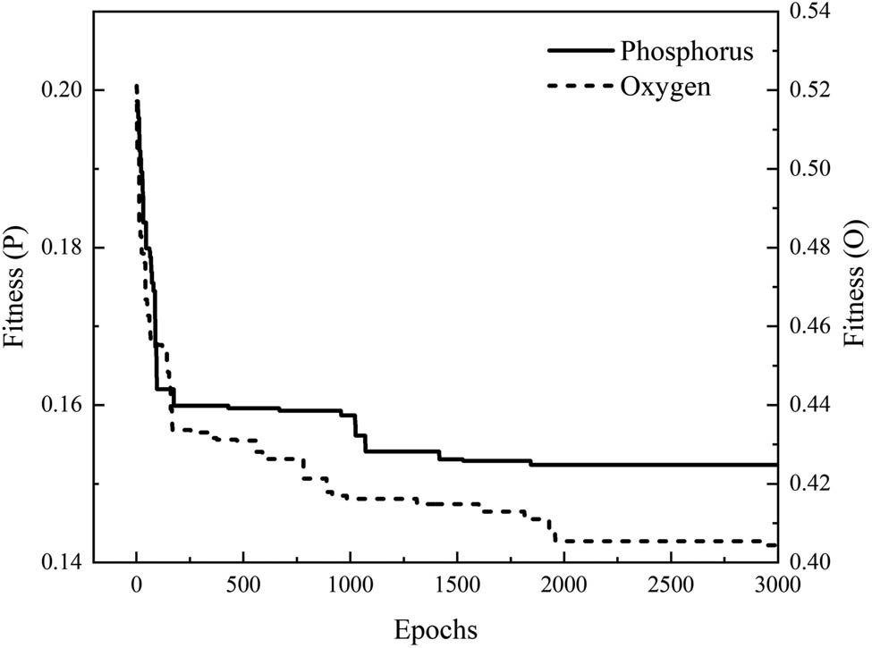
The error-epoch graph of GA–BP neural network.
3.4 Establishment of PCA–GA–BP neural network model
Through the above discussion, PCA is first used to reduce the dimensionality of the data, then GA is used to optimize the initialized weights and thresholds of the BP neural network, and finally, the structure of the BP neural network with PCA and GA is determined as 9 × 19 × 2 and 9 × 19 × 1.
3.5 Prediction results
The models of PCA–BP, GA–BP, and PCA–GA–BP are tested to make a comparison. Table 3 indicates the comparison of phosphorus content prediction accuracy of different models. The comparison between the single output model and the dual output model is also shown in the table. It is obvious that when the error is within ±0.005%, the hit rate of all models is 100%. The prediction accuracy of the model with single output is slightly higher than that of the same type of model with a dual output. At the same time, the PCA–GA–BP neural network model with single output exhibits higher prediction accuracy than that of other models.
Comparison of P content prediction accuracy of different models
| Model | Prediction error range (%) | ||||
|---|---|---|---|---|---|
| ±0.005 (%) | ±0.004 (%) | ±0.003 (%) | ±0.002 (%) | ±0.001 (%) | |
| PCA–BP (single) | 100 | 96 | 79 | 68 | 43 |
| PCA–BP (dual) | 100 | 96 | 85 | 63 | 34 |
| GA–BP (single) | 100 | 98 | 85 | 68 | 46 |
| GA–BP (dual) | 100 | 94 | 77 | 62 | 36 |
| PCA–GA–BP (single) | 100 | 98 | 94 | 84 | 72 |
| PCA–GA–BP (dual) | 100 | 93 | 76 | 62 | 37 |
The prediction accuracy of the oxygen content of different models is shown in Table 4. Similar to the prediction results of phosphorus content, the model with single output has higher accuracy than that with a dual output. Meanwhile, it is obvious that the PCA–GA–BP neural network with single output possesses the highest prediction accuracy.
Comparison of O content prediction accuracy of different models
| Model | Prediction error range (%) | ||||
|---|---|---|---|---|---|
| ±0.005 (%) | ±0.004 (%) | ±0.003 (%) | ±0.002 (%) | ±0.001 (%) | |
| PCA–BP (single) | 59 | 48 | 37 | 37 | 18 |
| PCA–BP (dual) | 53 | 46 | 34 | 26 | 15 |
| GA–BP (single) | 68 | 63 | 54 | 40 | 21 |
| GA–BP (Dual) | 67 | 61 | 53 | 34 | 16 |
| PCA–GA–BP (single) | 69 | 65 | 49 | 38 | 25 |
| PCA–GA–BP (dual) | 66 | 59 | 46 | 33 | 12 |
The reliability is low when the absolute error is used to evaluate the prediction accuracy of the model. For example, when the actual value of phosphorus content is less than 0.004%, the prediction error is 0.002%, and the deviation is more than 50%. Therefore, a relative error can accurately describe the accuracy of the prediction results, which is calculated using the formula:
where

Distribution of relative error within ±10%.
Moreover, in order to better compare the prediction accuracy, the performances of the models are evaluated by the root-mean-square error (RMSE) defined in equation (20).
The smaller the value of RMSE is, the better the model prediction performance is. The predictive performance of different models is analyzed and compared, as shown in Table 5. The RMSE of the single output model is lower than that of the dual output model. In other words, when single output is used by the model, its predictive performance is higher than when dual output is used. Therefore, it is advisable to build a single output model for predicting the phosphorus and oxygen contents of liquid steel, respectively.
RMSE (10−2) comparison of different models
| Model | Single output | Dual output | ||
|---|---|---|---|---|
| P | O | P | O | |
| PCA–BP | 0.21 | 0.64 | 0.21 | 0.68 |
| GA–BP | 0.19 | 0.53 | 0.22 | 0.54 |
| PCA–GA–BP | 0.15 | 0.49 | 0.22 | 0.58 |
The comparison between previous research and this study is shown in Table 6. In this study, when the error of phosphorus content is within 0.003%, the hit rate reaches 94%. By comparison, the prediction accuracy of the model in this study is higher than that of previous studies.
Comparison of prominent methods, deviations, hit rates and RMSE for phosphorus (P)
| Ref. | Method | P (%) | RMSE (%) |
|---|---|---|---|
| Wang et al. [6] | Weighted K-means and GMDH | ±0.004 | — |
| 88.4% | |||
| He and Zhang [7] | PCA–BP | ±0.004 | — |
| 92.06% | |||
| Bae et al. [8] | ANN | ±0.003 | — |
| 89% | |||
| Zhou et al. [9] | Monotone-constrained BP | ±0.003 | 0.0030 |
| 74% | |||
| Zhou et al. [10] | Grey correlation analysis–BP | ±0.004 | — |
| 83.33% | |||
| This study | PCA–GA–BP | ±0.003 | 0.0015 |
| 94% |
4 Conclusions
The present work established a BP neural network model to predict the end-point of BOF steelmaking, which is trained and tested by the data of 250t BOF. The bottom blowing and flux components are considered in the model to make the prediction accuracy higher. The following conclusions can be drawn:
By comparing single output model and dual output model, it is clear that the model with single output shows better predictive performance.
When the relative error is within ±10%, the hit rate of the PCA–GA–BP neural network with a single output for P and O contents reaches 83.0 and 80.0%, respectively.
The simulation experimental results show that the PCA–GA–BP neural network with single output has better regression capability than other models. The RMSE of P content between predicted and actual values is 0.0015%, and that of O content is 0.0049%. Therefore, the model can provide a good reference for BOF end-point control.
Acknowledgments
This work was financially supported by the National Natural Science Foundation of China (Grant no. 62071034).
-
Funding information: National Natural Science Foundation of China (Grant no. 62071034).
-
Author contributions: Shusen Cheng: writing the original draft; Zhao Liu: methodology and reviewing the document; Pengbo Liu: resources.
-
Conflict of interest: The authors state no conflict of interest.
-
Data availability statement: All authors can confirm that all data used in this article can be published in High Temperature Materials and Processes.
References
[1] Briant, C. L. and S. K. Banerji. Tempered martensite embrittlement in phosphorus doped steels. Metallurgical Transactions A, Vol. 10, No. 11, 1979, pp. 1729–1737.10.1007/BF02811708Search in Google Scholar
[2] Ogasawara, Y., Y. Miki, Y. Uchida, and N. Kikuchi. Development of high efficiency dephosphorization system in decarburization converter utilizing FetO dynamic control. ISIJ International, Vol. 5310, 2013, pp. 1786–1793.10.2355/isijinternational.53.1786Search in Google Scholar
[3] Tomiyama, S., Y. Uchida, H. Mizuno, K. Akiu, and T. Maeda. A novel control algorithm for dephosphorization in an LD converter. Journal of Process Control, Vol. 25, 2015, pp. 35–40.10.1016/j.jprocont.2014.11.002Search in Google Scholar
[4] Pal, S. and C. Halder. Optimization of phosphorous in steel produced by basic oxygen steel making process using multi-objective evolutionary and genetic algorithms. Steel Research International, Vol. 88, No. 3, 2017, id. 1600193.10.1002/srin.201600193Search in Google Scholar
[5] Lg, L. L., M. Ar, T. Kc, L. Hm, and O. Bj. Rapid prototyping tools for real-time expert systems in the steel industry. ISIJ International, Vol. 30, No. 2, 1990, pp. 90–97.10.2355/isijinternational.30.90Search in Google Scholar
[6] Wang, H. B., A. J. Xu, L. X. Ai, and N. Y. Tian. Prediction of endpoint phosphorus content of molten steel in BOF using weighted K-means and GMDH neural network. Journal of Iron and Steel Research International, Vol. 19, No. 1, 2012, pp. 11–16.10.1016/S1006-706X(12)60040-5Search in Google Scholar
[7] He, F. and L. Zhang. Prediction model of end-point phosphorus content in BOF steelmaking process based on PCA and BP neural network. Journal of Process Control, Vol. 66, 2018, pp. 51–58.10.1016/j.jprocont.2018.03.005Search in Google Scholar
[8] Bae, J., Y. Li, N. Ståhl, G. Mathiason, and N. Kojola. Using machine learning for robust target prediction in a Basic Oxygen Furnace system. Metallurgical and Materials Transactions B, Vol. 51, No. 4, 2020, pp. 1632–1645.10.1007/s11663-020-01853-5Search in Google Scholar
[9] Zhou, K. X., W. H. Lin, J. K. Sun, J. S. Zhang, D. Z. Zhang, X. M. Feng, et al. Prediction model of end-point phosphorus content for BOF based on monotone-constrained BP neural network. Journal of Iron and Steel Research International, Vol. 29, 2022, pp. 751–760.10.1007/s42243-021-00655-6Search in Google Scholar
[10] Zhou, C. G., J. Z. Hu, C. M. Jiang, S. H. Wang, L. Q. Ai, and H. Chen. Prediction model of phosphorus content in dephosphorization converter end point based on BP neural network algorithm. Steelmaking, Vol. 37, No. 2, 2021, pp. 10–15.Search in Google Scholar
[11] Wang, Z., J. Chang, Q.P. Ju, F. M. Xie, B. Wang, H. W. Li, et al. Prediction model of end-point manganese content for BOF steelmaking process. ISIJ International, Vol. 52, No. 9, 2012, pp. 1585–1590.10.2355/isijinternational.52.1585Search in Google Scholar
[12] Li, W., Q. M. Wang, X. S. Wang, and H. Wang. Endpoint prediction of BOF steelmaking based on BP neural network combined with improved PSO. Chemical Engineering Transactions, Vol. 51, 2016, pp. 475–480.Search in Google Scholar
[13] Gao, C., M. Shen, X. Liu, L. Wang, and M. Chen. End-point prediction of BOF steelmaking based on KNNWTSVR and LWOA. Transactions of the Indian Institute of Metals, Vol. 72, No. 1, 2019, pp. 257–270.10.1007/s12666-018-1479-5Search in Google Scholar
[14] Chen, Z. X., H. Liu, and L. Qi. Feature selection of BOF steelmaking process data by using an improved grey wolf optimizer. Journal of Iron and Steel Research International, Vol. 29, No. 8, 2022, pp. 1205–1223.10.1007/s42243-021-00673-4Search in Google Scholar
[15] Wang, Z., Q. Liu, H. Liu, and S. Wei. A review of end-point carbon prediction for BOF steelmaking process. High Temperature Materials and Processes, Vol. 39, No. 1, 2020, pp. 653–662.10.1515/htmp-2020-0098Search in Google Scholar
[16] Gu, M. Q., A. J. Xu, F. Yuan, X. M. He, and Z. F. Cui. An improved CBR model using time-series data for predicting the end-point of a converter. ISIJ International, Vol. 6110, 2021, pp. 2564–2570.10.2355/isijinternational.ISIJINT-2020-687Search in Google Scholar
[17] Zhou, H., Y. Hu, B. Wen, S. Wu, M. Kou, and Y. Luo. BP neural network prediction for Si and S contents in hot metal of COREX process based on mathematical analysis and Deng’s correlation. Metallurgical Research & Technology, Vol. 118, No. 5, 2021, id. 514.10.1051/metal/2021073Search in Google Scholar
[18] Kaike, C. Controlling oxygen activity in the molten steel at blowing end-point of BOF steelmaking. Iron and Steel, Vol. 44, No. 5, 2009, pp. 27–81.Search in Google Scholar
[19] Abdi, H. and L. J. Williams. Principal component analysis. Wiley interdisciplinary reviews: computational statistics, Vol. 2, No. 4, 2010, pp. 433–459.10.1002/wics.101Search in Google Scholar
[20] Werbos, P. J. The roots of backpropagation: from ordered derivatives to neural networks and political forecasting, 1, John Wiley & Sons, Inc., New York, NY, 1994.Search in Google Scholar
[21] Ding, S., C. Su, and J. Yu. An optimizing BP neural network algorithm based on genetic algorithm. Artificial Intelligence Review, Vol. 36, No. 2, 2011, pp. 153–162.10.1007/s10462-011-9208-zSearch in Google Scholar
[22] Xiangping, M., Z. Huaguang, and T. Wanyu. A hybrid method of GA and BP for short-term economic dispatch of hydrothermal power systems. Mathematics and Computers in Simulation, Vol. 51, No. 3–4, 2000, pp. 341–348.10.1016/S0378-4754(99)00128-7Search in Google Scholar
[23] Rivera, W. A. and P. Xanthopoulos. A priori synthetic over-sampling methods for increasing classification sensitivity in imbalanced data sets. Expert Systems with Applications, Vol. 66, 2016, pp. 124–135.10.1016/j.eswa.2016.09.010Search in Google Scholar
[24] Chen, J., M. Mahfouf, and G. Sidahmed. A new holistic systems approach to the design of heat treated alloy steels using a biologically inspired multi-objective optimisation algorithm. Engineering Applications of Artificial Intelligence, Vol. 37, 2015, pp. 103–114.10.1016/j.engappai.2014.08.014Search in Google Scholar
[25] Chen, C., N. Wang, and M. Chen. Prediction model of end-point phosphorus content in consteel electric furnace based on PCA-extra tree model. ISIJ International, Vol. 61, No. 6, 2021, pp. 1908–1914.10.2355/isijinternational.ISIJINT-2020-615Search in Google Scholar
[26] Cybenko, G. Approximation by superpositions of a sigmoidal function. Mathematics of Control, Signals and Systems, Vol. 2, No. 4, 1989, pp. 303–314.10.1007/BF02551274Search in Google Scholar
[27] Hornik, K., M. Stinchcombe, and H. White. Multilayer feedforward networks are universal approximators. Neural networks, Vol. 2, No. 5, 1989, pp. 359–366.10.1016/0893-6080(89)90020-8Search in Google Scholar
[28] Hecht-Nielsen, R. Neurocomputing, Addison-Wesley, Menlo Park, CA, 1990.Search in Google Scholar
© 2022 Zhao Liu et al., published by De Gruyter
This work is licensed under the Creative Commons Attribution 4.0 International License.
Articles in the same Issue
- Research Articles
- Numerical and experimental research on solidification of T2 copper alloy during the twin-roll casting
- Discrete probability model-based method for recognition of multicomponent combustible gas explosion hazard sources
- Dephosphorization kinetics of high-P-containing reduced iron produced from oolitic hematite ore
- In-phase thermomechanical fatigue studies on P92 steel with different hold time
- Effect of the weld parameter strategy on mechanical properties of double-sided laser-welded 2195 Al–Li alloy joints with filler wire
- The precipitation behavior of second phase in high titanium microalloyed steels and its effect on microstructure and properties of steel
- Development of a huge hybrid 3D-printer based on fused deposition modeling (FDM) incorporated with computer numerical control (CNC) machining for industrial applications
- Effect of different welding procedures on microstructure and mechanical property of TA15 titanium alloy joint
- Single-source-precursor synthesis and characterization of SiAlC(O) ceramics from a hyperbranched polyaluminocarbosilane
- Carbothermal reduction of red mud for iron extraction and sodium removal
- Reduction swelling mechanism of hematite fluxed briquettes
- Effect of in situ observation of cooling rates on acicular ferrite nucleation
- Corrosion behavior of WC–Co coating by plasma transferred arc on EH40 steel in low-temperature
- Study on the thermodynamic stability and evolution of inclusions in Al–Ti deoxidized steel
- Application on oxidation behavior of metallic copper in fire investigation
- Microstructural study of concrete performance after exposure to elevated temperatures via considering C–S–H nanostructure changes
- Prediction model of interfacial heat transfer coefficient changing with time and ingot diameter
- Design, fabrication, and testing of CVI-SiC/SiC turbine blisk under different load spectrums at elevated temperature
- Promoting of metallurgical bonding by ultrasonic insert process in steel–aluminum bimetallic castings
- Pre-reduction of carbon-containing pellets of high chromium vanadium–titanium magnetite at different temperatures
- Optimization of alkali metals discharge performance of blast furnace slag and its extreme value model
- Smelting high purity 55SiCr automobile suspension spring steel with different refractories
- Investigation into the thermal stability of a novel hot-work die steel 5CrNiMoVNb
- Residual stress relaxation considering microstructure evolution in heat treatment of metallic thin-walled part
- Experiments of Ti6Al4V manufactured by low-speed wire cut electrical discharge machining and electrical parameters optimization
- Effect of chloride ion concentration on stress corrosion cracking and electrochemical corrosion of high manganese steel
- Prediction of oxygen-blowing volume in BOF steelmaking process based on BP neural network and incremental learning
- Effect of annealing temperature on the structure and properties of FeCoCrNiMo high-entropy alloy
- Study on physical properties of Al2O3-based slags used for the self-propagating high-temperature synthesis (SHS) – metallurgy method
- Low-temperature corrosion behavior of laser cladding metal-based alloy coatings on EH40 high-strength steel for icebreaker
- Study on thermodynamics and dynamics of top slag modification in O5 automobile sheets
- Structure optimization of continuous casting tundish with channel-type induction heating using mathematical modeling
- Microstructure and mechanical properties of NbC–Ni cermets prepared by microwave sintering
- Spider-based FOPID controller design for temperature control in aluminium extrusion process
- Prediction model of BOF end-point P and O contents based on PCA–GA–BP neural network
- Study on hydrogen-induced stress corrosion of 7N01-T4 aluminum alloy for railway vehicles
- Study on the effect of micro-shrinkage porosity on the ultra-low temperature toughness of ferritic ductile iron
- Characterization of surface decarburization and oxidation behavior of Cr–Mo cold heading steel
- Effect of post-weld heat treatment on the microstructure and mechanical properties of laser-welded joints of SLM-316 L/rolled-316 L
- An investigation on as-cast microstructure and homogenization of nickel base superalloy René 65
- Effect of multiple laser re-melting on microstructure and properties of Fe-based coating
- Experimental study on the preparation of ferrophosphorus alloy using dephosphorization furnace slag by carbothermic reduction
- Research on aging behavior and safe storage life prediction of modified double base propellant
- Evaluation of the calorific value of exothermic sleeve material by the adiabatic calorimeter
- Thermodynamic calculation of phase equilibria in the Al–Fe–Zn–O system
- Effect of rare earth Y on microstructure and texture of oriented silicon steel during hot rolling and cold rolling processes
- Effect of ambient temperature on the jet characteristics of a swirl oxygen lance with mixed injection of CO2 + O2
- Research on the optimisation of the temperature field distribution of a multi microwave source agent system based on group consistency
- The dynamic softening identification and constitutive equation establishment of Ti–6.5Al–2Sn–4Zr–4Mo–1W–0.2Si alloy with initial lamellar microstructure
- Experimental investigation on microstructural characterization and mechanical properties of plasma arc welded Inconel 617 plates
- Numerical simulation and experimental research on cracking mechanism of twin-roll strip casting
- A novel method to control stress distribution and machining-induced deformation for thin-walled metallic parts
- Review Article
- A study on deep reinforcement learning-based crane scheduling model for uncertainty tasks
- Topical Issue on Science and Technology of Solar Energy
- Synthesis of alkaline-earth Zintl phosphides MZn2P2 (M = Ca, Sr, Ba) from Sn solutions
- Dynamics at crystal/melt interface during solidification of multicrystalline silicon
- Boron removal from silicon melt by gas blowing technique
- Removal of SiC and Si3N4 inclusions in solar cell Si scraps through slag refining
- Electrochemical production of silicon
- Electrical properties of zinc nitride and zinc tin nitride semiconductor thin films toward photovoltaic applications
- Special Issue on The 4th International Conference on Graphene and Novel Nanomaterials (GNN 2022)
- Effect of microstructure on tribocorrosion of FH36 low-temperature steels