Understanding the Factors Influencing the Number of Extracurricular Clubs in American High Schools
-
Amy Tang


Abstract
Previous research has provided compelling evidence of a strong connection between extracurricular activities and positive youth development. While both school offerings and student participation affect the outcomes of extracurricular activities, earlier studies have primarily focused on student participation. In contrast, this study shifts the focus to school offerings. We extensively collect lists of extracurricular clubs offered by hundreds of American high schools and analyze the relationship between schools’ club counts and various factors, such as school enrollment, household income, pupil-to-teacher ratio, and racial demographics. We find that, although the relationship exhibits complex higher-order effects and nonlinearity, it can still be effectively captured by our carefully constructed predictive model. Moreover, we find that, despite the significant influence of school demographics, schools still have ample opportunities to take the initiative to improve their club offerings.
1 Introduction
American Youths have been active in extracurricular activities (Mahoney, Harris, & Eccles, 2006), and the past studies have provided compelling evidence of a strong connection between positive youth development and active engagement in organized extracurricular activities (Buckley & Lee, 2021; Feraco, Resnati, Fregonese, Spoto, & Meneghetti, 2023; Heath, Anderson, Turner, & Payne, 2022; Mkude & Mubofu, 2022; Leksuwankun, Dangprapai, & Wangsaturaka, 2023; Busseri, Rose-Krasnor, Willoughby, & Chalmers, 2006; Gilman, Meyers, & Perez, 2004; Eccles, Barber, Stone, & Hunt, 2003; Marsh & Kleitman, 2002; Feldman & Matjasko, 2005; Darling, Caldwell, & Smith, 2005; Eccles & Templeton, 2002; Gardner, Roth, J., & Brooks-Gunn, 2008; Fredricks & Eccles, 2006; Reeves, 2008; Fredricks & Eccles, 2006; Fredricks & Eccles, 2005; Peck, Roeser, Zarrett, & Eccles, 2008). Participation in such activities has been found to be linked to a reduction in problem behaviors and an improvement in academic performance (Mahoney, Larson, & Eccles, 2005; Anjum, 2021; Mukesh, Acharya, & Pillai, 2023). Furthermore, these advantages may extend into young adulthood, predicting academic achievements and fostering prosocial behaviors (Zaff, Moore, Papillo, & Williams, 2003). More recently, extracurricular activities have also been found to help prevent social networks addiction (Borrego & Cuadrado, 2025).
The benefits of high school extracurricular clubs are rooted in several foundational learning theories. Interest-based learning theory (Dewey & Wheeler, 1913) asserts that students learn most effectively when education aligns with their interests and incorporates active, hands-on experiences. Self-determination theory (Deci & Ryan, 2012) suggests that individuals are motivated to learn and grow when they experience autonomy, competence, and relatedness. Social learning theory (Bandura & Walters, 1977) underscores the role of observation and imitation in the learning process, while the situated learning theory (Lave, 1991) emphasizes that learning occurs through participation in communities of practice, engaging in authentic activities. Finally, the expectancy-value theory (Wigfield & Eccles, 2000) highlights that individuals’ beliefs about their abilities and the value they assign to a task influence their motivation and performance. Extracurricular clubs align closely with these theories by catering to students’ interests, fostering autonomy in self-organization, providing opportunities to observe, practice, and collaborate within a community, and enhancing confidence through successful experiences in activities that match their interests.
Given the importance of extracurricular clubs in student development, researchers have studied factors influencing participation for over half a century. However, significant gaps remain, which this study seeks to address.
First, previous studies have primarily examined the “demand side” of the student–school relationship, focusing on student participation. These studies typically survey individual students and analyze how factors such as school size (Kleinert, 1969; McNeal, 1999) and socioeconomic status (Feldman & Matjasko, 2007) influence participation rates. In contrast, this study takes a different approach by focusing on the “supply side,” specifically the number of clubs offered by different schools and the impact of various factors (e.g., school enrollment, household income, pupil-to-teacher ratio, and racial demographics) on the club count. This previously overlooked supply-side information is important because, for example, among schools with similar enrollment and socioeconomic status, one offering significantly fewer clubs (i.e., fewer supplies) may experience reduced student participation rates, regardless of students’ potential interest (i.e., potential demand).
Second, previous studies often rely on data collected from only a few schools through in-person surveys, resulting in insufficient data to draw statistically significant conclusions. In contrast, leveraging the public data accessibility in the Internet era, this study adopts a novel approach to collect and clean club data from hundreds of schools’ websites. This dataset, which is two orders of magnitude larger than those in previous studies, enables a more comprehensive and in-depth analysis.
Third, previous studies in social science often assume a simple linear relationship between predictors (e.g., a school’s club count) and independent variables (e.g., school enrollment and socioeconomic status), typically relying on correlation analysis. However, we find that higher-order effects and nonlinearity are present among the factors we study. Empowered by the larger dataset, this study holistically evaluates various linear and nonlinear models to identify the one that most accurately captures the complex relationship among these factors.
In the following sections, we describe how this study addresses gaps identified in the previous research. Before delving into the details, we briefly summarize the key findings for ease of reference:
The factors influencing the number of clubs offered by schools, ranked by impact, are school size, household income, and pupil-to-teacher ratio.
After accounting for their indirect influence through school size and household income, racial demographics do not significantly affect club count.
The number of clubs offered by a school is correlated with
Schools with a lower pupil-to-teacher ratio tend to offer more clubs.
Lower-income schools tend to offer fewer clubs, but this effect flattens out when
Among schools with similar demographics (enrollment, household income, and pupil-to-teacher ratio), the top quartile offers 3.2 times more clubs than the bottom quartile, emphasizing the pivotal role of individual school initiatives.
2 Methodology for Data Collection
American high schools are secondary schools typically covering grades 9–12. Nearly every high school offers certain school-sponsored extracurricular clubs overseen by the school administration. These clubs provide students with opportunities to engage in a wide variety of activities, including STEM (e.g., robotics), career path (e.g., Future Farmers of America), arts (e.g., drama), social issues (e.g., LGBTQ+ rights), student association (e.g., Black Student Union), leadership and community service (e.g., Key Club), political awareness (e.g., Junior State of America), competition (e.g., Model United Nations), school-community building (e.g., newspaper), culture (e.g., Chinese traditional clothing), intramural sports (e.g., mountain biking), hobbies (e.g., chess), and religions (e.g., Catholicism).
The quantity and variety of clubs provided by high schools are influenced by various factors, ultimately affecting students’ participation. For instance, smaller schools might struggle to gather enough students interested in starting a Latin club, while larger schools might have a surplus of students vying for club leadership positions, resulting in the overmanning effect (Barker & Gump, 1964). Moreover, schools with a high pupil-to-teacher ratio, indicating fewer teachers, may struggle to find a teacher with the necessary bandwidth or expertise to oversee a specific club. Finally, schools predominantly composed of students from lower-income families might face financial constraints preventing the establishment of clubs like robotics.
We collected a substantial amount of data to analyze the impact of various factors on schools’ club counts. Specifically, we used data from the American National Center for Education Statistics (NCES) (NCES, 2023) for information about school sizes, free or reduced-price lunch, pupil-to-teacher ratios, and racial demographics. In addition, we collected complete lists of clubs offered by many schools.
Of all the American public schools that have data reported by NCES for the school year 2021–2022, we selected high schools for this study based on the following criteria. We excluded schools that do not offer grade 12 and only counted students in grades 9–12. Throughout the rest of this article, the term “students” only refers to grade 9–12 students in a school, excluding students from other grades, if present. We focused on physical schools and excluded virtual schools. In addition, we excluded private schools. Finally, we excluded schools that provided no information about their free or reduced-price lunch program, as well as schools that did not report their pupil-to-teacher ratio. This resulted in a total of 21,064 schools that enrolled a total of 14,030,023 grade 9–12 students. We refer to these schools as “candidate schools” or “all schools” throughout the rest of this article.
2.1 Sampling of Schools
We first present the characteristics of schools, followed by a description of our school sampling methodology. Figure 1 shows the cumulative distribution of school count and student count as a function of school size. The “all schools” curves represent the 21,064 schools. The “sampled schools” curves represent 229 schools that were randomly selected from the 21,064 schools for this study. We will describe the selection of these schools later.
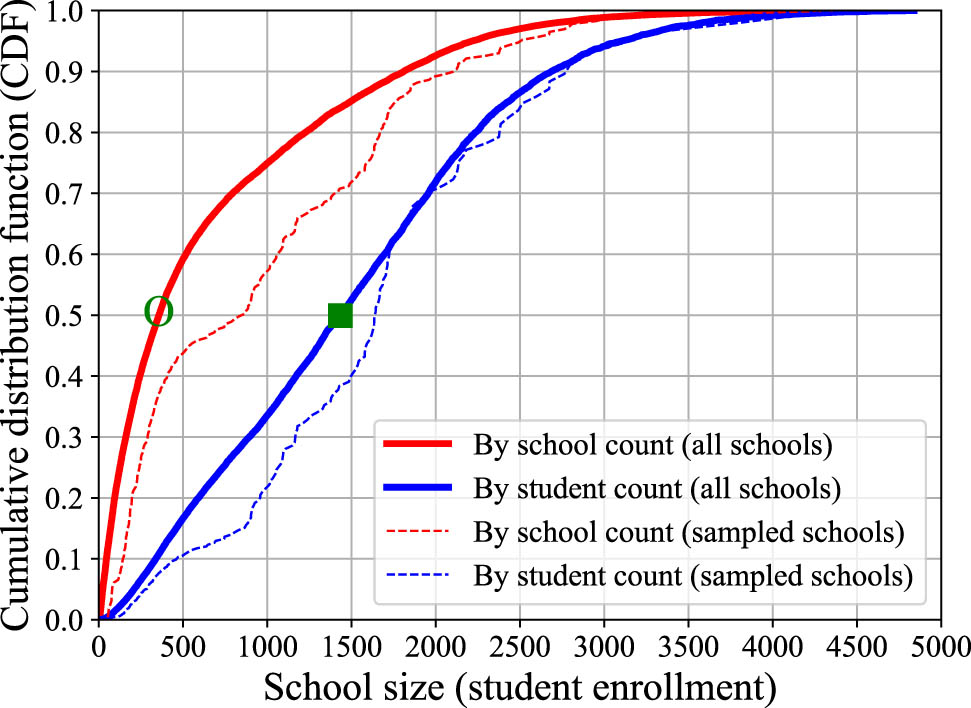
Cumulative distribution of school count and student count as functions of school size. While most schools are small, most students attend larger schools. To avoid a uniform sample dominated by small schools, we intentionally oversampled larger ones.
As an example of how to read the figure, the data point in the green circle on the “by school count (all schools)” curve means that 50% (see the Y-axis) of all schools have 357 (see the X-axis) or fewer students. Similarly, the data point in the green square on the “by student count (all schools)” curve means that 50% of all students across all schools are enrolled in schools that each have 1,434 or fewer students.
These data highlight a significant divergence between school count and student count. While the majority of schools are small, the majority of students are enrolled in larger schools. This affects how we select the sampled schools. Initially, we selected the sampled schools in a way that ensured, in Figure 1, the curve of “by school count (sampled schools)” closely matched the curve of “by school count (all schools).” However, this led to a lack of sufficient data points for large schools because small schools make up the majority. Specifically, schools with 1,000 or fewer students account for 75% of all schools while hosting only 34% of all students. To address this issue, we intentionally sampled more schools of larger sizes. This leads to the divergence of the “all schools” curves and the “sampled schools” curves in the figure. We will delve further into this topic during the data analysis.
2.2 Collecting Club Data
The NCES data contain no information about extracurricular clubs offered by schools. To collect such data, traditional approaches would typically resort to surveys to contact individuals at specific schools, with approvals from numerous ethics committees. However, this approach is challenging to scale to hundreds of schools nationwide, which might be a key reason why, after more than half a century of research on extracurricular activities, there are still no publicly available large-scale datasets providing complete lists of clubs offered by many schools.
In the Internet era, we instead take an innovative approach to collect club data from schools’ public websites. Interestingly, the shift to online learning during the COVID-19 pandemic facilitated this data collection process, as an increasing number of schools have adopted websites as a primary channel for communication.
Specifically, we sampled thousands of schools, searched their respective websites, and identified 229 schools with complete lists of clubs they offer. It is important to note that while many school websites include information about a limited subset of clubs as examples, they do not present a comprehensive list of all available clubs. We have excluded these schools from our study. On average, it takes searching through more than 15 schools to identify one with sufficiently complete club data. Consequently, we conducted searches across thousands of schools to identify the 229 sampled schools. In total, the 229 schools hosted 221,300 students and offered 5,983 clubs.
Among a school’s clubs, this study excludes clubs for varsity sports such as swimming and baseball for two reasons: (1) They form a substantial category on their own and merit a separate, dedicated study, and (2) the treatment of varsity sports on school websites is highly inconsistent. While some schools classify them as clubs, others categorize them separately under athletics. Furthermore, common varsity sports are frequently not reported on websites despite the likelihood that most schools offer them. For the sake of maintaining consistency in this study, we have excluded varsity sports and intend to explore them in future work. However, we do include intramural sports in this study, such as trapshooting and mountain biking, as they tend to be consistently reported as clubs on different school websites. Similarly, we excluded student councils and class-specific clubs such as Class 2025 because almost every school has these clubs, but the practice of whether to include them as clubs on school websites is inconsistent.
As several co-authors extracted club data from school websites, one challenge was ensuring inter-rater consistency. To address this, we established clear rules to exclude certain schools (e.g., private schools) and adopted a two-step process. First, a software tool randomly sampled thousands of schools from the NCES dataset. Co-authors then searched for each school’s website, identified the specific pages listing club data, and excluded schools that listed only a subset of clubs as examples rather than presenting a comprehensive list of all available clubs. This step filtered out approximately 95% of the sampled schools, leaving around 250. In the second step, a single evaluator reviewed the club webpages of the approximately 250 remaining schools and further excluded any that appeared to have incomplete club data, resulting in a final set of 229 schools. Having a single evaluator performing the second step ensured consistency and avoided inter-rater discrepancies in the final list. The process is scalable, as over 95% of the effort occurred in the first step, which was parallelized across multiple co-authors. A limitation, however, is that some valid schools may have been prematurely excluded in the first step by different data collectors, without a chance for the final evaluator to review them – potentially introducing bias and reducing the dataset size.
3 Data Analysis and Findings
In this section, we analyze the effect of various factors on the number of clubs offered by schools. For convenience, the variables used in our analysis are summarized in Table 1, and the basic school statistics are summarized in Table 2.
Symbols for dependent and independent variables used in this study
| Variable | Explanation |
|---|---|
|
|
Number of clubs offered by a school |
|
|
School size, i.e., student enrollment |
|
|
Pupil-to-teacher ratio. A higher
|
|
|
Fraction of students in a school receiving free or reduced-price lunch. A higher
|
|
|
Fraction of students of a specific race in a school |
Average school statistics. For example, the “White” column shows that, among all 21,064 schools, 45.45% of students are White, while among the 229 sampled schools, 41.57% of students are White. This table shows that the sampled schools are representative in terms of racial demographics
| Variable |
|
|
|
White (%) | Hispanic (%) | Black (%) | Asian/Pacific Islander (%) | Multi-race (%) | Native American (%) | Hawaiian or other Pacific Isl. (%) |
|---|---|---|---|---|---|---|---|---|---|---|
| All schools | 666 | 50 | 15.0 | 45.45 | 28.80 | 15.03 | 5.48 | 3.92 | 0.88 | 0.38 |
| Sampled schools | 966 | 47 | 15.3 | 41.57 | 31.36 | 14.10 | 7.91 | 4.02 | 0.56 | 0.41 |
Our goal is to develop a multiple regression model for predicting the number of clubs (
3.1 Effect of School Size
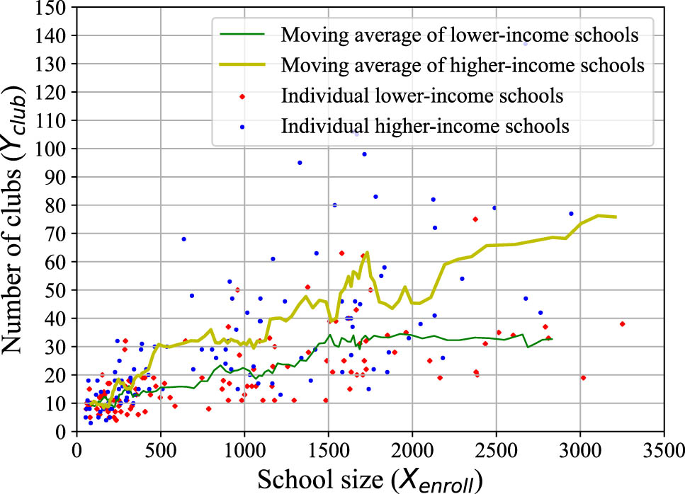
Our analysis starts with the school size factor. For an initial intuitive grasp of the effect of school size, we plot in Figure 2 the relationship between school size (
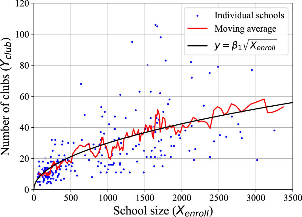
The number of clubs follows the trend of square root of school size. Without thorough modeling and exploration of different curve-fitting functions, one might oversimplify the relationship between school size and number of clubs, mistakenly assuming a linear correlation that could lead to suboptimal results.
The moving-average curve reveals a strong positive correlation between
The moving-average curve in Figure 2 shows that
This function is also plotted in Figure 2, showing good alignment with the moving-average curve. Note that we fit the function to the entire dataset instead of the moving-average curve, which merely aids visualization.
We derive several observations from Figure 2. First, the simplicity of the function is appealing, indicating a square root relationship between
In Figure 2, one might note that a big fraction of the sampled schools are relatively small, i.e., with 500 or fewer students. This is because most schools are smaller schools, as shown by the curve of “by school count (all schools)” in Figure 1. To have sufficient samples for larger schools, we already intentionally sampled a bigger fraction of larger schools, as shown by the curve of “by school count (sampled schools)” in Figure 1.
Finally, from Figure 2, one might be inclined to assume that students at smaller schools are at a disadvantage, given their schools offer fewer clubs. However, Figure 3 presents a contrasting perspective, unveiling that the number of clubs per student is, in fact, higher in smaller schools. Because the number of clubs follows the trend of
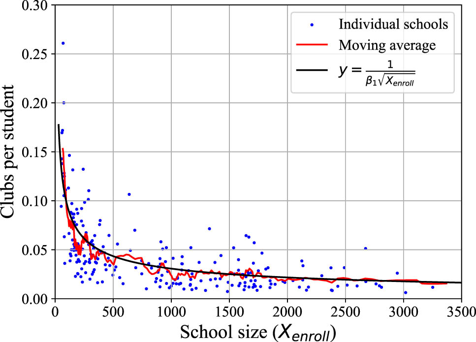
The number of clubs per student decreases as the school size increases. On the one hand, smaller schools tend to have fewer clubs, limiting students’ choices. On the other hand, students at smaller schools enjoy better opportunities for leadership roles and active club engagement.
3.2 Effect of Pupil-to-Teacher Ratio
In addition to school size, the pupil-to-teacher ratio (
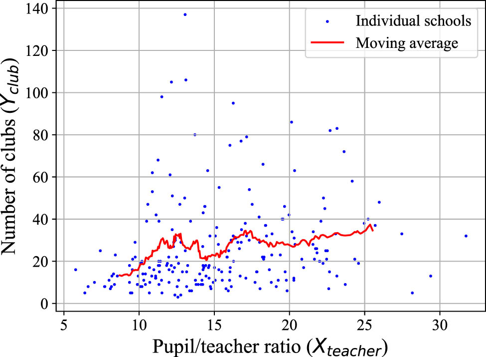
Schools with higher
Further investigation reveals that this counterintuitive result is merely a side effect of the correlation between
To assess the true effect of
To prevent this, we follow the division lines in Figure 6 to create school groups for comparison. Specifically, we first sort the schools by their sizes. For every 30 adjacent schools in the sorted list with similar school sizes, we identify division lines that divide the 30 schools into three groups of equal sizes with higher, medium, and lower
Partition the 229 sampled schools into three groups based on their
We compare the higher- and lower-
Schools in the lower-
Furthermore, Figure 7 illustrates that the gap in
3.3 Effect of Household Income
Next, we analyze the effect of household income by using
To assess whether we need to exclude the influence of school size before analyzing the effect of
Figure 8 illustrates the relationship between
Only when
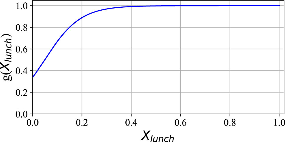
This logistic function
Because of the nonlinear relationship between
Overall, because the curve in Figure 8 flattens out when
To further quantify the statistical significance of the effect of household income, we follow the method shown in Figure 6 to partition the 229 sampled schools into three groups based on the values of
Higher-income schools tend to have more clubs.
Similar to Figures 7 and 10 also shows that the disparity in
3.4 Effect of Racial Demographics
In this section, we analyze the effect of racial demographics. We begin by examining the largest racial group, the White students. For each school, we compute the fraction of White students as
Since both
The resulting higher- and lower-
To visualize the pattern, we plot the schools in the higher- and lower-
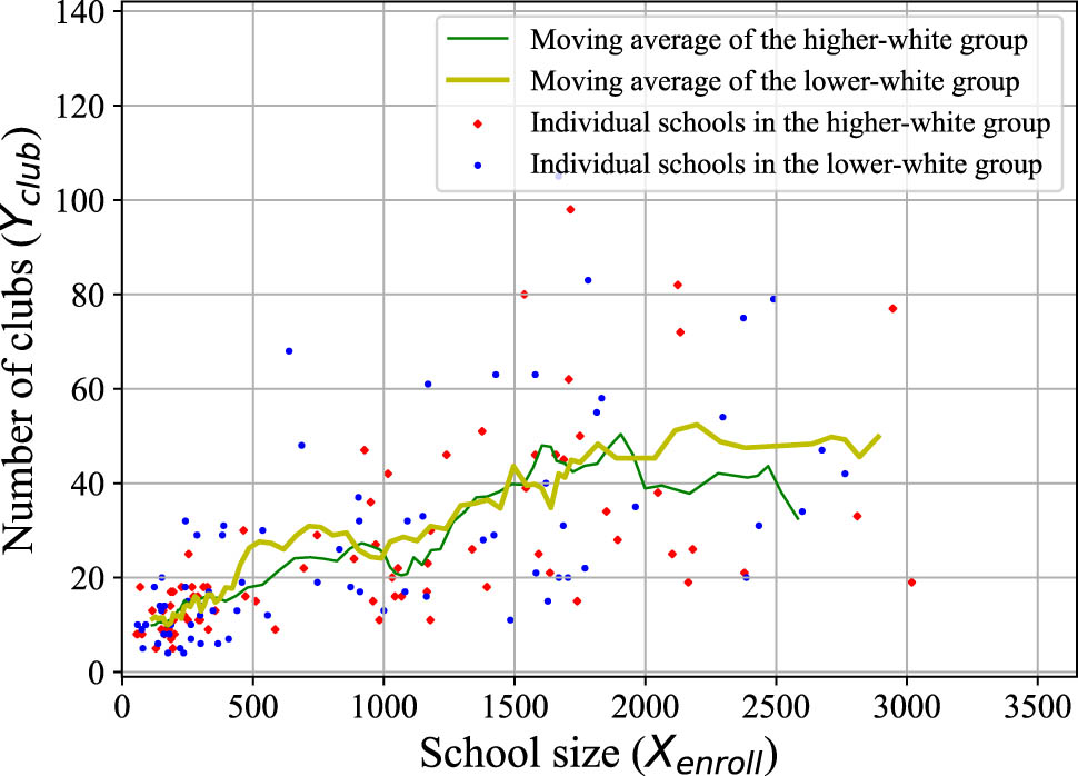
For two school groups with comparable
Similar
Results of
|
|
|
White (
|
Hispanic | Black | Asian/Pacific Islander | Multirace | Native American | Hawaiian/other Pacific Isl. | |
|---|---|---|---|---|---|---|---|---|---|
| Difference in mean |
|
|
|
5.4 |
|
0.1 | 0.0 |
|
|
|
|
|
|
|
1.59 |
|
0.03 |
|
|
|
|
|
|
|
0.5203 | 0.114 | 0.6103 | 0.9792 | 0.9955 | 0.1922 | 0.6271 |
The
3.5 Multiple Regression Model
After understanding the characteristics of individual independent variables, in this section, we design a multiple regression model that incorporates all the factors. Specifically, we model the number of clubs as
where
A distinctive aspect of this model is the role of
In addition to this model, we have explored numerous others, including those incorporating additional terms related to
3.6 Further Simplifying the Model
Although the model in equation (3) seems intuitive and comprehensive, we find that the terms representing racial demographics,
We use the linear regression implementation in the statsmodels package (Statsmodels, 2023) to compute the coefficients. Information concerning these coefficients is summarized in Table 4. Due to the presence of heteroscedasticity in the residual, as evident in Figures 7 and 10, we employ the HC3 covariance matrix estimator in statsmodels to calculate heteroskedasticity-robust standard errors. This estimator implements the algorithm proposed by MacKinnon and White (MacKinnon & White, 1985).
Information about the model coefficients in equation (5).
| Coefficient symbol | Coefficient value | Robust standard error |
|
|
Confidence interval | Partial
|
|
|---|---|---|---|---|---|---|---|
| [0.025 | 0.975] | ||||||
|
|
3.2124 | 0.333 | 9.66 |
|
2.557 | 3.868 | 0.50 |
|
|
|
0.298 |
|
|
|
|
0.30 |
|
|
|
0.008 |
|
|
|
|
0.08 |
The adjusted
The mean of the model residual,
The signs of the coefficients in Table 4 align with the previous analysis results for individual variables. Specifically,
After establishing the simplified model in equation (5) as a solid baseline, we delve into the reasoning behind excluding the
These observations indicate that the inclusion of
3.7 School Initiatives in Improving Club Offerings
On the one hand, the multiple regression model’s reasonable accuracy, with an adjusted
To illustrate the substantial effect of school initiatives, we compare top- and bottom-performing schools in terms of club offerings in Figure 12. For each school, we calculate the ratio between its actual club count and the club count prediction derived from equation (5). A school with a higher ratio outperforms a school with a lower ratio. In Figure 12, we plot the top and bottom 1/4 schools with the highest and lowest values in this ratio, respectively. This figure reveals a significant disparity between the top and bottom schools. Specifically, the average of the ratios for the top 1/4 schools is 163%, whereas that for the bottom 1/4 schools is only 51%. In other words, the top schools have 3.2 times more clubs than the bottom schools after school demographics are taken into account, emphasizing the pivotal role of individual school initiatives.
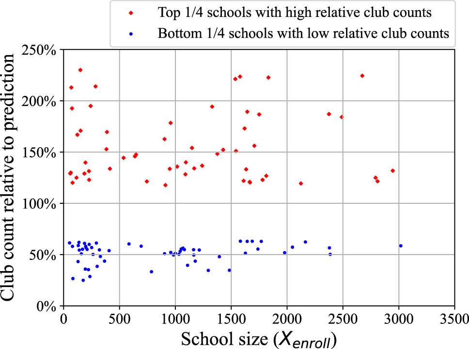
Out of the 229 sampled schools, this figure compares the relative club counts between the top 58 schools and the bottom 58 schools. After accounting for school demographics, the top and bottom schools still show a significant difference in club count, emphasizing the pivotal role of individual school initiatives.
3.8 Analysis Summary and Lessons Learned
Overall, the simplified model demonstrates a reasonable level of accuracy, indicated by its adjusted
A valuable lesson we have learned is that the design of this model greatly benefited from a thorough initial analysis of the characteristics of individual variables, rather than blindly including them in a linear regression model. This aided us in identifying and designing the aforementioned features of the model.
In contrast, if the traditional linear regression model shown below were used, it would produce misleading and unreasonable results despite its seemingly acceptable
Specifically, the regression result for the aforementioned model misleadingly suggests that
Another valuable lesson we have learned is that when validating observations, we have frequently strived to design experiments that directly compare two population groups differing significantly in one independent variable while maintaining similar characteristics across other independent variables. Concrete examples include the comparisons shown in Figures 7, 10, and 11, which are further summarized in Table 3. This direct validation approach has enhanced our confidence in and improved our interpretation of the summaries generated by statistical software.
4 Discussion and Recommendation
In this section, we discuss issues that may adversely affect the availability of clubs provided by schools, starting with the school size factor, as it has the biggest affect due to its multiplicative role in equation (3). The challenge is evident in Figure 3, which shows a decrease in club opportunity per student as school size increases. In particular, large schools experience the over-manning effect (Barker & Gump, 1964), resulting in a surplus of students competing for club leadership positions, which limits opportunities for leadership skill development. Moreover, as club growth lags behind student enrollment, increased student-to-club ratios discourage participation. These observations align with the prior research indicating lower student engagement in various activities within larger schools (Schoggen & Schoggen, 1988,Morgan & Alwin, 1980,Stevens & Peltier, 1994).
What limits club growth in larger schools? One hypothesis is that, since the pupil-to-teacher ratio tends to be higher in larger schools, as illustrated in Figure 5, the availability of teachers as supervisors for clubs might be a limiting factor. However, Figure 13 contradicts this. As the club opportunity per student decreases with school size, the club support load per teacher similarly decreases, implying teachers are not the bottleneck. In this figure, the moving average curves are computed similarly to those in Figure 2, but individual schools are not plotted to avoid overcrowding the figure. Club support load per teacher is calculated as
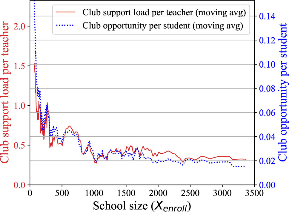
Club support load per teacher decreases as school size increases.
We believe that the inclination to eliminate redundant clubs is a contributing factor that negatively affects club offerings, leading to the emergence of large clubs and the subsequent over-manning effect, ultimately discouraging participation. Comparing club offerings to course offerings, we observe that in large schools, popular courses such as algebra often offer multiple parallel classes to reduce class size and promote engagement. However, this approach is seldom applied to clubs, even though clubs like chess and Key Club are popular. Despite the theoretical possibility of dividing large clubs into smaller subgroups for internal operations, this is rarely practiced. In addition, the number of club officers rarely increases in proportion to club size. These factors naturally restrict club size and diminish participation rates in larger schools. Furthermore, national organizations like Key Club usually establish one chapter per school, inadvertently causing the chapter to become unwieldy in larger schools, further dissuading participation.
We propose extending the practice applied to courses to clubs. In large schools, it would be advantageous to establish multiple clubs of the same category, such as multiple chess clubs or Key Club chapters, each with independent club officers. This approach would provide leadership opportunities to a larger pool of students, who subsequently can work with the student community to boost participation rates. In addition, we recommend encouraging the creation of similar clubs with slight variations in focus. Notably, large schools successful in offering many clubs tend to feature numerous community service clubs, each centered around a slightly distinct theme. Conversely, certain schools enforce policies discouraging the establishment of new clubs similar to existing ones, inadvertently leading to the overmanning effect and reduced participation.
Our recommendation takes a more moderate stance compared to Leithwood and Jantzi’s recommendation to cap secondary schools at 1,000 students or fewer (Leithwood & Jantzi, 2009). Fourteen years after their initial proposal, schools with 1,000 or fewer students host only 34% of the total student population (Figure 1), and the trend of school consolidation remains unaltered. We suggest working within the existing school structure and introducing smaller, immediately actionable changes with substantial potential, instead of waiting for major school demographics to shift, which could take decades to occur.
Besides our more actionable approach to coping with the hard-to-change school size factor, in general, we strongly advocate for individual schools taking initiatives to improve club offerings despite the constraints of school demographics. Specifically, Figure 12 shows that the top 1/4 schools have 3.2 times more clubs than the bottom 1/4 schools after school demographics are taken into account, emphasizing the pivotal role of individual school initiatives. Besides these statistics, there are also concrete examples. One inspiring example is Syracuse Academy of Science Charter School (Syracuse, 2023). Despite having only 286 students, with 75% of them receiving free or reduced-price lunch, the school boasts an impressive 29 clubs, which is several times higher than that of similar schools. The school’s focus on science is reflected in its numerous STEM-related clubs, but it also offers a diverse range of clubs encompassing humanity, charity, arts, and hobbies.
The statement from Principal Corey Tafoya of Woodstock High School, which had successfully improved the student participation rate in extracurricular activities by over 400% in five years, encapsulates our recommendation most effectively: “If we have six or seven students interested in something, we’ll start a new club. We want students to find a reason to get up and come to school. Whatever trips their trigger is what our teachers and administration are willing to do” (Reeves, 2008).
5 Limitations and Future Work
One limitation of this research is that it collects samples from school websites, which could lead to biased outcomes, as it excludes schools that do not publish club data online. Despite this limitation, it is considered an acceptable tradeoff for the first attempt, given the constraints of alternative methods for gathering comprehensive club data. For instance, conducting in-person surveys would likely introduce bias toward schools willing to participate in this type of study, and achieving widespread coverage across hundreds of schools dispersed throughout the United States would be challenging. Other limitations include the exclusion of varsity sports clubs and private schools from this study, which are subjects for future research.
6 Related Works
The past research has presented compelling evidence of a strong association between positive youth development and active involvement in extracurricular activities, as supported by various studies (Mkude & Mubofu, 2022; Leksuwankun, Benítez, Albertos, & Lara, 2023; Balaguer et al., 2020a; Busseri et al., 2006; Gilman et al., 2004; Eccles et al., 2003; Marsh & Kleitman, 2002; Darling et al., 2005; Eccles & Templeton, 2002; Mahoney et al., 2005; Zaff et al., 2003; Lerner et al., 2005; Gardner et al., 2008; Reeves, 2008; Fredricks & Eccles, 2006; Fredricks & Eccles, 2005; Peck et al., 2008). In addition, several surveys have summarized the effects of participation in extracurricular activities (Seow & Pan, 2014; Feldman & Matjasko, 2005; Holland & Andre, 1987; Farb & Matjasko, 2012; Rahayu & Dong, 2023). Specifically, it has been shown that positive parenting is associated with success in extracurricular activities and the development of personality traits (Balaguer et al., 2020b). Finally, a prominent taxonomy, known as “the five Cs,” attributes the positive outcomes to the beneficial effect of organized extracurricular activities on five key areas of youth development: competence, confidence, connection, character, and caring (Lerner et al., 2005).
It is important to note that, while there is evidence of a strong association between positive youth development and extracurricular activities, some studies argue that factors other than the quantity and variety of activities offered by a school – such as peer relations, sense of belonging, perceived support, and school climate – play a more important role (Balaguer, Benítez, de la Fuente, & Osorio, 2022; Hamlin, 2021; Berhanu & Sewagegn, 2024).
Concerns about the over-scheduled child problem have been raised in some studies (Rosenfeld & Wise, 2010). However, Mahoney et al. conducted an extensive survey and supported promoting participation in extracurricular activities, as they found limited empirical support for the overscheduling hypothesis and consistent evidence for the positive youth development perspective (Mahoney et al., 2006).
Some research suggests that the benefits of extracurricular activities may depend, in part, on the type of activities in which youth participate (Marsh & Kleitman, 2002; Larson, Hansen, & Moneta, 2006). Fredricks & Eccles (2006) examined the effect of the total number and breadth of participation in activities on youth development. These studies assume that a reasonable number and variety of extracurricular clubs are available to students. Related to this assumption, this research examines factors influencing the availability of high school clubs.
Barker and Gump’s study on school size and available extracurricular activities is relevant to this research (Barker & Gump, 1964). However, their work was limited to data from a small number of schools in a specific region (13 high schools in Eastern Kansas) and was conducted about half a century ago. In contrast, our modern research is more comprehensive, encompassing 229 schools spread across the United States, and considering factors beyond just school size.
McNeal’s study (McNeal, 1999) is also related to this research, as it investigated the effect of school size and pupil-to-teacher ratio on student participation in high school extracurricular activities. However, in terms of the student–school relationship, this research focuses on the supply side of extracurricular clubs offered by high schools, in contrast to McNeal’s emphasis on the demand side, specifically student participation. Similarly, some work primarily focuses on factors affecting non-participators, such as lower socioeconomic status, lower grades, and larger schools (Feldman & Matjasko, 2007).
Various studies have discussed the effects of large school sizes, including their affect on student indiscipline (Haller, 1992), dropout rates (Alspaugh, 1998), voluntary participation (Schoggen & Schoggen, 1988), social participation (Morgan & Alwin, 1980), and social networks (Schaefer, Simpkins, Vest, & Price, 2011). Stevens and Peltier conducted a literature review and found support for the claim that students in smaller schools are more actively involved in extracurricular activities than students in larger schools (Stevens & Peltier, 1994). Our quantification of the
7 Conclusion
By using data collected from hundreds of American high schools, we have studied the factors that impact schools’ club counts, which ultimately affect students’ participation rates in club activities. Our findings are summarized below.
First, the number of clubs offered by a school follows the trend of
Second, using the fraction of students in a school receiving free or reduced-price lunch, denoted as
Third, at first glance, there seems to be a positive correlation between the pupil-to-teacher ratio and the number of clubs, implying that a decrease in the number of teachers leads to an increase in the number of clubs. However, this counterintuitive outcome is primarily due to schools with higher pupil-to-teacher ratios mostly being large schools, which generally offer more clubs. Once the influence of school size is excluded, the number of clubs exhibits a negative correlation with the pupil-to-teacher ratio. Specifically, a controlled experiment shows that among schools of comparable sizes, schools with lower pupil-to-teacher ratios, on average, have 9.3 more clubs than those with higher pupil-to-teacher ratios.
Fourth, at first glance, racial demographics seem to affect the number of clubs, as they are correlated with school size and household income, which directly affect the number of clubs. However, after excluding their indirect influence through school size and household income, racial demographics by themselves do not significantly affect the number of clubs. Specifically, both
Fifth, our analysis reveals that for schools with identical demographic characteristics – such as school size, household income, and pupil-to-teacher ratio – the top 25% of schools offer 3.2 times more clubs than the bottom 25%. This notable difference underscores the crucial role of school initiatives in increasing club offerings.
In summary, the factors influencing the number of clubs offered by schools, ranked by impact, are school size, household income, and pupil-to-teacher ratio, while racial demographics do not significantly affect club count. Finally, despite demographic constraints such as school size, schools still have ample opportunities to take the initiative to improve club offerings.
Acknowledgments
The authors are grateful for the reviewers’ valuable comments that improved the manuscript.
-
Funding information: The authors state no funding involved.
-
Author contributions: All authors take responsibility for the entire content of this manuscript, have consented to its submission to the journal, reviewed all the results, and approved the final version of the manuscript. A.T. conceived the original idea for this study. A.T. and C.T. collected the data and performed the analysis. Y.W. proposed the multiple-regression method. All authors contributed to the writing and finalization of the manuscript.
-
Conflict of interest: The authors state no conflict of interest.
-
Data availability statement: The data will be provided upon request to the authors.
References
Alspaugh, J. W. (1998). The relationship of school-to-school transitions and school size to high school dropout rates. The High School Journal, 81(3), 154–160. Search in Google Scholar
Anjum, S. (2021). Impact of extracurricular activities on academic performance of students at secondary level. International Journal of Applied Guidance and Counseling, 2(2), 7–14. 10.26486/ijagc.v2i2.1869Search in Google Scholar
Balaguer, A., Benítez, E., Albertos, A., & Lara, S. (2020a). Not everything helps the same for everyone: Relevance of extracurricular activities for academic achievement. Humanities and Social Sciences Communications, 7(1), 1–8. 10.1057/s41599-020-00573-0Search in Google Scholar
Balaguer, A., Benítez, E., de la Fuente, J., & Osorio, A. (2022). Structural empirical model of personal positive youth development, parenting, and school climate. Psychology in the Schools, 59(3), 451–470. 10.1002/pits.22620Search in Google Scholar
Balaguer, A., Orejudo, S., Rodriguez-Ledo, C., & Cardoso-Moreno, M. J. (2020b). Extracurricular activities, positive parenting and personal positive youth development. Differential relations amongst age and academic pathways. Electronic Journal of Research in Educational Psychology, 2(18), 179–206. 10.25115/ejrep.v18i51.2929Search in Google Scholar
Bandura, A. & Walters, R. H. (1977). Social learning theory. Englewood Cliffs, NJ: Prentice Hall. Search in Google Scholar
Barker, R. G., & Gump, P. V. (1964). Big school, small school: High school size and student behavior. Redwood City, CA: Stanford University Press. Search in Google Scholar
Berhanu, K. Z., & Sewagegn, A. A. (2024). The role of perceived campus climate in students’ academic achievements as mediated by students engagement in higher education institutions. Cogent Education, 11(1), 2377839. 10.1080/2331186X.2024.2377839Search in Google Scholar
Borrego, I., & Cuadrado, I. (2025). Extracurricular activities for adolescents to prevent social networks addiction. American Research Journal of Humanities Social Science, 8(2), 57–63. Search in Google Scholar
Buckley, P., & Lee, P. (2021). The impact of extra-curricular activity on the student experience. Active Learning in Higher Education, 22(1), 37–48. 10.1177/1469787418808988Search in Google Scholar
Busseri, M. A., Rose-Krasnor, L., Willoughby, T., & Chalmers, H. (2006). A longitudinal examination of breadth and intensity of youth activity involvement and successful development. Developmental Psychology, 42(6), 1313. 10.1037/0012-1649.42.6.1313Search in Google Scholar
Darling, N., Caldwell, L. L., & Smith, R. (2005). Participation in school-based extracurricular activities and adolescent adjustment. Journal of Leisure Research, 37(1), 51–76. 10.1080/00222216.2005.11950040Search in Google Scholar
Deci, E. L., & Ryan, R. M. (2012). Self-determination theory. Handbook of Theories of Social Psychology, 1(20), 416–436. 10.4135/9781446249215.n21Search in Google Scholar
Dewey, J., & Wheeler, J. E. (1913). Interest and effort in education. Boston: Houghton Mifflin. 10.1037/14633-000Search in Google Scholar
Eccles, J. S., Barber, B. L., Stone, M., & Hunt, J. (2003). Extracurricular activities and adolescent development. Journal of Social Issues, 59(4), 865–889. 10.1046/j.0022-4537.2003.00095.xSearch in Google Scholar
Eccles, J. S., & Templeton, J. (2002). Chapter 4: Extracurricular and other after-school activities for youth. Review of Research in Education, 26(1), 113–180. 10.3102/0091732X026001113Search in Google Scholar
Farb, A. F., & Matjasko, J. L. (2012). Recent advances in research on school-based extracurricular activities and adolescent development. Developmental Review, 32, 1–48. 10.1016/j.dr.2011.10.001Search in Google Scholar
Feldman, A. F., & Matjasko, J. L. (2005). The role of school-based extracurricular activities in adolescent development: A comprehensive review and future directions. Review of Educational Research, 75(2), 159–210. 10.3102/00346543075002159Search in Google Scholar
Feldman, A. F., & Matjasko, J. L. (2007). Profiles and portfolios of adolescent school-based extracurricular activity participation. Journal of Adolescence, 30(2), 313–332. 10.1016/j.adolescence.2006.03.004Search in Google Scholar
Feraco, T., Resnati, D., Fregonese, D., Spoto, A., & Meneghetti, C. (2023). An integrated model of school students’ academic achievement and life satisfaction. linking soft skills, extracurricular activities, self-regulated learning, motivation, and emotions. European Journal of Psychology of Education, 38(1), 109–130. 10.1007/s10212-022-00601-4Search in Google Scholar
Fredricks, J. A., & Eccles, J. S. (2005). Developmental benefits of extracurricular involvement: Do peer characteristics mediate the link between activities and youth outcomes? Journal of Youth and Adolescence, 34, 507–520. 10.1007/s10964-005-8933-5Search in Google Scholar
Fredricks, J. A., & Eccles, J. S. (2006). Extracurricular involvement and adolescent adjustment: Impact of duration, number of activities, and breadth of participation. Applied Developmental Science, 10(3), 132–146. 10.1207/s1532480xads1003_3Search in Google Scholar
Gardner, M., Roth, J., & Brooks-Gunn, J. (2008). Adolescents’ participation in organized activities and developmental success 2 and 8 years after high school: Do sponsorship, duration, and intensity matter? Developmental Psychology, 44(3), 814. 10.1037/0012-1649.44.3.814Search in Google Scholar
Gilman, R., Meyers, J., & Perez, L. (2004). Structured extracurricular activities among adolescents: Findings and implications for school psychologists. Psychology in the Schools, 41(1), 31–41. 10.1002/pits.10136Search in Google Scholar
Haller, E. J. (1992). High school size and student indiscipline: Another aspect of the school consolidation issue? Educational Evaluation and Policy Analysis, 14(2), 145–156. 10.3102/01623737014002145Search in Google Scholar
Hamlin, D. (2021). Can a positive school climate promote student attendance? evidence from new york city. American Educational Research Journal, 58(2), 315–342. 10.3102/0002831220924037Search in Google Scholar
Heath, R. D., Anderson, C., Turner, A. C., & Payne, C. M. (2022). Extracurricular activities and disadvantaged youth: A complicated but promising story. Urban Education, 57(8), 1415–1449. 10.1177/0042085918805797Search in Google Scholar
Holland, A., & Andre, T. (1987). Participation in extracurricular activities in secondary school: What is known, what needs to be known? Review of Educational Research, 57, 437–466. 10.3102/00346543057004437Search in Google Scholar
Kleinert, E. J. (1969). Effects of high school size on student activity participation. The Bulletin of the National Association of Secondary School Principals, 53(335), 34–46. 10.1177/019263656905333506Search in Google Scholar
Larson, R. W., Hansen, D. M., & Moneta, G. B. (2006). Differing profiles of developmental experiences across types of organized youth activities. Developmental Psychology, 42(5), 849–863. 10.1037/0012-1649.42.5.849Search in Google Scholar
Lave, J. (1991). Situated learning: Legitimate peripheral participation. Cambridge: Cambridge University Press. 10.1017/CBO9780511815355Search in Google Scholar
Leithwood, K., & Jantzi, D. (2009). A review of empirical evidence about school size effects: A policy perspective. Review of Educational Research, 79(1), 464–490. 10.3102/0034654308326158Search in Google Scholar
Leksuwankun, S., Dangprapai, Y., & Wangsaturaka, D. (2023). Student engagement in organising extracurricular activities: Does it matter to academic achievement? Medical Teacher, 45(3), 272–278. 10.1080/0142159X.2022.2128733Search in Google Scholar
Lerner, R. M., Lerner, J. V., Almerigi, J. B., Theokas, C., Phelps, E., Gestsdottir, S., …, von Eye, A. (2005). Positive youth development, participation in community youth development programs, and community contributions of fifth-grade adolescents: Findings from the first wave of the 4-h study of positive youth development. The Journal of Early Adolescence, 25(1), 17–71. 10.1177/0272431604272461Search in Google Scholar
MacKinnon, J. G., & White, H. (1985). Some heteroskedasticity-consistent covariance matrix estimators with improved finite sample properties. Journal of Econometrics, 29(3), 305–325. 10.1016/0304-4076(85)90158-7Search in Google Scholar
Mahoney, J. L., Harris, A. L., & Eccles, J. S. (2006). Organized activity participation, positive youth development, and the over-scheduling hypothesis. Social Policy Report, 20(4), 3–30. 10.1002/j.2379-3988.2006.tb00049.xSearch in Google Scholar
Mahoney, J. L., Larson, R. W., & Eccles, J. S. (2005). Organized activities as contexts of development: Extracurricular activities, after school and community programs. London, England: Psychology Press. 10.4324/9781410612748Search in Google Scholar
Marsh, H., & Kleitman, S. (2002). Extracurricular school activities: The good, the bad, and the nonlinear. Harvard Educational Review, 72(4), 464–515. 10.17763/haer.72.4.051388703v7v7736Search in Google Scholar
McNeal Jr, R. B. (1999). Participation in high school extracurricular activities: Investigating school effects. Social Science Quarterly, 80(2), 291–309. Search in Google Scholar
Mkude, M., & Mubofu, C. (2022). Extracurricular activities in the broader personal development: Reflections from youth in public secondary schools. Research Ambition: An International Multidisciplinary e-Journal, 6(IV), 1–5. 10.53724/ambition/v6n4.02Search in Google Scholar
Morgan, D. L., & Alwin, D. F. (1980). When less is more: School size and student social participation. Social Psychology Quarterly, 43(2), 241–252. 10.2307/3033627Search in Google Scholar
Mukesh, H. V., Acharya, V., & Pillai, R. (2023). Are extracurricular activities stress busters to enhance students well-being and academic performance? Evidence from a natural experiment. Journal of Applied Research in Higher Education, 15(1), 152–168. 10.1108/JARHE-06-2021-0240Search in Google Scholar
NCES. (2023). National Center for Education Statistics. https://nces.ed.gov/ccd/elsi/tableGenerator.aspx. Search in Google Scholar
Peck, S. C., Roeser, R. W., Zarrett, N., & Eccles, J. S. (2008). Exploring the roles of extracurricular activity quantity and quality in the educational resilience of vulnerable adolescents: Variable-and pattern-centered approaches. Journal of Social Issues, 64(1), 135–156. 10.1111/j.1540-4560.2008.00552.xSearch in Google Scholar
Rahayu, A. P., & Dong, Y. (2023). The relationship of extracurricular activities with students’ character education and influencing factors: a systematic literature review. Al-Ishlah: Jurnal Pendidikan, 15(1), 459–474. 10.35445/alishlah.v15i1.2968Search in Google Scholar
Reeves, D. B. (2008). The learning leader/the extracurricular advantage. Learning, 66(1), 86–87. Search in Google Scholar
Rosenfeld, A., & Wise, N. (2010). The over-scheduled child: Avoiding the hyper-parenting trap. New York: St. Martinas Griffin. Search in Google Scholar
Schaefer, D. R., Simpkins, S. D., Vest, A. E., & Price, C. D. (2011). The contribution of extracurricular activities to adolescent friendships: New insights through social network analysis. Developmental Psychology, 47(4), 1141–1152. 10.1037/a0024091Search in Google Scholar
Schoggen, P., & Schoggen, M. (1988). Student voluntary participation and high school size. The Journal of Educational Research, 81(5), 288–293. 10.1080/00220671.1988.10885837Search in Google Scholar
Seow, P.-S., & Pan, G. (2014). A literature review of the impact of extracurricular activities participation on students’ academic performance. Journal of Education for Business, 89(7), 361–366. 10.1080/08832323.2014.912195Search in Google Scholar
Statsmodels. (2023). https://www.statsmodels.org/. Search in Google Scholar
Stevens, N. G., & Peltier, G. L. (1994). A review of research on small-school student participation in extracurricular activities. Journal of Research in Rural Education, 10(2), 116–120. Search in Google Scholar
Syracuse. (2023). Syracuse Academy of Science Charter School, NCES school ID 360010405549, list of clubs: https://www.sascs.org/students-parents/student-activities. Search in Google Scholar
Wigfield, A., & Eccles, J. S. (2000). Expectancy-value theory of achievement motivation. Contemporary Educational Psychology, 25(1), 68–81. 10.1006/ceps.1999.1015Search in Google Scholar
Zaff, J. F., Moore, K. A., Papillo, A. R., & Williams, S. (2003). Implications of extracurricular activity participation during adolescence on positive outcomes. Journal of Adolescent Research, 18(6), 599–630. 10.1177/0743558403254779Search in Google Scholar
© 2025 the author(s), published by De Gruyter
This work is licensed under the Creative Commons Attribution 4.0 International License.
Articles in the same Issue
- Special Issue: Disruptive Innovations in Education - Part II
- Formation of STEM Competencies of Future Teachers: Kazakhstani Experience
- Technology Experiences in Initial Teacher Education: A Systematic Review
- Ethnosocial-Based Differentiated Digital Learning Model to Enhance Nationalistic Insight
- Delimiting the Future in the Relationship Between AI and Photographic Pedagogy
- Research Articles
- Examining the Link: Resilience Interventions and Creativity Enhancement among Undergraduate Students
- The Use of Simulation in Self-Perception of Learning in Occupational Therapy Students
- Factors Influencing the Usage of Interactive Action Technologies in Mathematics Education: Insights from Hungarian Teachers’ ICT Usage Patterns
- Study on the Effect of Self-Monitoring Tasks on Improving Pronunciation of Foreign Learners of Korean in Blended Courses
- The Effect of the Flipped Classroom on Students’ Soft Skill Development: Quasi-Experimental Study
- The Impact of Perfectionism, Self-Efficacy, Academic Stress, and Workload on Academic Fatigue and Learning Achievement: Indonesian Perspectives
- Revealing the Power of Minds Online: Validating Instruments for Reflective Thinking, Self-Efficacy, and Self-Regulated Learning
- Culturing Participatory Culture to Promote Gen-Z EFL Learners’ Reading Proficiency: A New Horizon of TBRT with Web 2.0 Tools in Tertiary Level Education
- The Role of Meaningful Work, Work Engagement, and Strength Use in Enhancing Teachers’ Job Performance: A Case of Indonesian Teachers
- Goal Orientation and Interpersonal Relationships as Success Factors of Group Work
- A Study on the Cognition and Behaviour of Indonesian Academic Staff Towards the Concept of The United Nations Sustainable Development Goals
- The Role of Language in Shaping Communication Culture Among Students: A Comparative Study of Kazakh and Kyrgyz University Students
- Lecturer Support, Basic Psychological Need Satisfaction, and Statistics Anxiety in Undergraduate Students
- Parental Involvement as an Antidote to Student Dropout in Higher Education: Students’ Perceptions of Dropout Risk
- Enhancing Translation Skills among Moroccan Students at Cadi Ayyad University: Addressing Challenges Through Cooperative Work Procedures
- Socio-Professional Self-Determination of Students: Development of Innovative Approaches
- Exploring Poly-Universe in Teacher Education: Examples from STEAM Curricular Areas and Competences Developed
- Understanding the Factors Influencing the Number of Extracurricular Clubs in American High Schools
- Student Engagement and Academic Achievement in Adolescence: The Mediating Role of Psychosocial Development
- The Effects of Parental Involvement toward Pancasila Realization on Students and the Use of School Effectiveness as Mediator
- A Group Counseling Program Based on Cognitive-Behavioral Theory: Enhancing Self-Efficacy and Reducing Pessimism in Academically Challenged High School Students
- A Significant Reducing Misconception on Newton’s Law Under Purposive Scaffolding and Problem-Based Misconception Supported Modeling Instruction
- Product Ideation in the Age of Artificial Intelligence: Insights on Design Process Through Shape Coding Social Robots
- Navigating the Intersection of Teachers’ Beliefs, Challenges, and Pedagogical Practices in EMI Contexts in Thailand
- Business Incubation Platform to Increase Student Motivation in Creative Products and Entrepreneurship Courses in Vocational High Schools
- On the Use of Large Language Models for Improving Student and Staff Experience in Higher Education
- Coping Mechanisms Among High School Students With Divorced Parents and Their Impact on Learning Motivation
- Twenty-First Century Learning Technology Innovation: Teachers’ Perceptions of Gamification in Science Education in Elementary Schools
- Exploring Sociological Themes in Open Educational Resources: A Critical Pedagogy Perspective
- Teachers’ Emotions in Minority Primary Schools: The Role of Power and Status
- Investigating the Factors Influencing Teachers’ Intention to Use Chatbots in Primary Education in Greece
- Working Memory Dimensions and Their Interactions: A Structural Equation Analysis in Saudi Higher Education
- A Practice-Oriented Approach to Teaching Python Programming for University Students
- Reducing Fear of Negative Evaluation in EFL Speaking Through Telegram-Mediated Language Learning Strategies
- Demographic Variables and Engagement in Community Development Service: A Survey of an Online Cohort of National Youth Service Corps Members
- Educational Software to Strengthen Mathematical Skills in First-Year Higher Education Students
- The Impact of Artificial Intelligence on Fostering Student Creativity in Kazakhstan
- Review Articles
- Current Trends in Augmented Reality to Improve Senior High School Students’ Skills in Education 4.0: A Systematic Literature Review
- Exploring the Relationship Between Social–Emotional Learning and Cyberbullying: A Comprehensive Narrative Review
- Determining the Challenges and Future Opportunities in Vocational Education and Training in the UAE: A Systematic Literature Review
- Socially Interactive Approaches and Digital Technologies in Art Education: Developing Creative Thinking in Students During Art Classes
- Current Trends Virtual Reality to Enhance Skill Acquisition in Physical Education in Higher Education in the Twenty-First Century: A Systematic Review
- Understanding the Technological Innovations in Higher Education: Inclusivity, Equity, and Quality Toward Sustainable Development Goals
- Perceived Teacher Support and Academic Achievement in Higher Education: A Systematic Literature Review
- Mathematics Instruction as a Bridge for Elevating Students’ Financial Literacy: Insight from a Systematic Literature Review
- STEM as a Catalyst for Education 5.0 to Improve 21st Century Skills in College Students: A Literature Review
- A Systematic Review of Enterprise Risk Management on Higher Education Institutions’ Performance
- Case Study
- Contrasting Images of Private Universities