Time-varying Investment Dynamics in the USA
-
Ivan Mendieta-Muñoz


Abstract
We study the time-varying effects of Tobin’s q and cash flow on investment dynamics in the USA using a vector autoregression model with drifting parameters and stochastic volatilities estimated via Bayesian methods. We find a significant variation over time of the response of investment to shocks in both variables. The time-varying sensitivity of investment to a shock in Tobin’s q (cash flow) decreased (increased) since the early 1960s through the early 1980s, increased (decreased) since the early 1980s through the early 2000s, and it has decreased (increased) importantly again since then. Thus, the time-varying response of investment to a shock to Tobin’s q has been almost the mirror image to the time-varying response of investment to a shock to cash flow. This implies that Tobin’s q and cash flow represent both complementary and alternative sources of information needed to understand short-run investment behavior.
1 Introduction
The theoretical and empirical literature on aggregate investment has emphasized two features of utmost importance regarding its behavior: (i) that its dynamics are heavily influenced by Tobin’s q and cash flow; and (ii) that the investment sensitivities to both variables can vary dynamically and non-linearly over time.
First, aggregate investment is an increasing function of average Tobin’s q – the market valuation of a firm divided by the replacement cost of its capital stock – because this variable measures the average return on firms’ capital anticipated by the market, thus representing a proxy for the availability of external equity finance that influences firms’ investment expectations and decisions.
Second, aggregate investment is also an increasing function of cash flow since the latter captures the availability of internal funds, which are crucial for managing large and growing firms, as well as for financing new investment opportunities that firms deem potentially attractive.
Third, the relationship between investment, Tobin’s q, and cash flow does not seem to be static or stable over time because of the reasons associated with changes in adjustment costs, financial constraints, and technological improvements. This implies that dynamic non-linear models represent highly relevant avenues of research in order to provide a more comprehensive understanding of the behavior of aggregate investment over time.[1]
In this article, we present the first study on the evolution of the time-varying sensitivities of aggregate investment to Tobin’s q and cash flow in the USA that considers a multiple equation model designed to capture time variation in the dynamic structural linkages among the variables as well as the possible time variation in the volatilities (heteroskedasticity) of the shocks. To do so, we estimate a time-varying parameter vector autoregression model with stochastic volatility (TVP-VAR-SV model) via Bayesian methods, along the lines of Del Negro and Primiceri (2015) and Primiceri (2005). Our empirical model (i) allows for a flexible strategy to study the possible time-varying behavior of the underlying structure of investment dynamics in a multivariate framework, (ii) allows for a structural interpretation of the dynamic responses of investment to changes in Tobin’s q and cash flow, and (iii) controls for the time-varying volatilities of the shocks over time.
Our main findings for the post-World War II period can be summarized as follows. First, we find significant evidence of time variation in the response of investment to shocks in Tobin’s q and cash flow, which highlights the existence of relevant structural changes in the dynamics of investment and its linkages to both variables.
Second, the time-varying response of investment to a shock to Tobin’s q is almost the mirror image to the time-varying response of investment to a shock to cash flow. Specifically, the time-varying sensitivity of investment to a shock in Tobin’s q decreased since the early 1960s through the early 1980s, increased since the early 1980s through the early 2000s, and it has tended to decrease importantly again since then. On the other hand, the time-varying sensitivity of investment to a shock in cash flow increased since the early 1960s through the early 1980s, decreased since the early 1980s through the early 2000s, and it has tended to increase importantly again since then. Such time-varying patterns in the investment sensitivities to Tobin’s q and cash flow are mainly observed in the short run, especially within the first 2 years after the initial shocks.
Hence, our results suggest that although Tobin’s q and cash flow represent complementary sources of information for investment dynamics because both variables influence simultaneously firms’ investment decisions, their relative importance for the latter has changed considerably over time, so that Tobin’s q and cash flow should also be regarded as alternative sources of information for short-run investment fluctuations.
The remainder of this article is organized as follows. A review of the literature that helps to motivate the current research is presented in Section 2. Section 3 presents the relevant data and discusses some stylized facts that additionally motivate the use of a TVP-VAR-SV model to study the dynamics of aggregate investment. The model and the empirical methodology are summarized in Section 4. Section 5 summarizes the main results, and, finally, the main conclusions are presented in Section 6.
2 Related Literature and Contribution
This contribution is mainly related to the theoretical and empirical literature that has emphasized that investment depends dynamically and non-linearly on variables associated with liquidity and finance constraints.
According to the original q theory of investment (Tobin, 1969), corporate investment is an increasing function of average Tobin’s q because, in equilibrium, the firms’ combined market value should be equal to their replacement costs – Tobin’s q ratio should be equal to 1 in equilibrium. A low Tobin’s q ratio – between 0 and 1 – can be regarded as an indicator that the cost to replace the firms’ assets is greater than the value of the stocks, so the stocks are undervalued. By contrast, a high Tobin’s q ratio – greater than 1 – can be considered as an indicator that the stocks are overvalued since the cost to replace the firms’ assets is lower than the value of the stocks. Therefore, Tobin’s q represents a variable that approximates the availability of external equity finance, which affects firms’ investment decisions mainly via investment expectations.
However, since Tobin’s q is an imperfect variable that regularly fails to control for the entire investment opportunity set, aggregate investment is also an increasing function of cash flow, i.e., a variable that captures the availability of internal funds. Different theories have been proposed to explain the positive relationship between investment decisions and cash flow, including the existence of agency problems (see, e.g., Grabowski & Mueller, 1972, among others) and asymmetric information (see, e.g., Stiglitz & Weiss, 1981, among others).[2]
The existence of agency problems assumes that managers obtain financial and psychological gains from managing a large and growing firm, thus investing beyond the point that maximizes shareholder wealth. Although external capital sources could be used, internal funds are expected to be favored in this situation because they are the most accessible part of the capital market and are most malleable to managerial desires for growth. This also implies that a greater percentage of internal funds are retained and invested than are warranted to maximize shareholder welfare.
On the other hand, the existence of asymmetric information emphasizes that firms with attractive investment opportunities may be unable to finance their investment decisions because the cost of external funds can be too high due to the capital market’s ignorance of firms’ investment opportunities. If this occurs, firms with inadequate internal cash flows will not be able to finance their investment expenditures when needed; however, firms with large cash flows will be better prepared to finance their new investment opportunities.
In the same vein, the more recent theoretical models developed by Abel and Eberly (2011, 2012), and Lettau and Ludvigson (2002) articulate different possibilities to understand the simultaneous and potentially changing relationships between investment, Tobin’s q, and cash flow. To sum up, this strand of literature has shown three important results. First, there are significant dynamic interactions that can change over time between investment and Tobin’s q – for instance, because discount rates are not constant (Lettau & Ludvigson, 2002).
Second, even if other adjustment costs and financial constraints are eliminated, it can be shown that investment still remains sensitive to both Tobin’s q and cash flow (Abel & Eberly, 2011).
Third, when growth options that vary over time are considered – which occurs because the firm’s level of productivity is a choice variable, investment is positively correlated with cash flow during intervals of time between consecutive technology upgrades, but investment would be uncorrelated with Tobin’s q during such intervals. However, the positive correlation between investment and Tobin’s q is essentially associated with the forward-looking nature of the value of the firm, which can also change over time (Abel & Eberly, 2012).
At the empirical level, recent contributions have explored the possible changes over time of the sensitivity of investment to Tobin’s q and cash flow, mainly at the microlevel by considering firm-level data. Ağca and Mozumdar (2008), Brown and Petersen (2009), and Chen and Chen (2012) use US manufacturing firm data for the periods 1970–2001, 1970–2006, and 1967–2006, respectively. Ağca and Mozumdar (2008) controlled for other factors associated with capital market imperfections – namely, fund flows, institutional ownership, analyst following, bond ratings, and an index of antitakeover amendments, finding a steady decline in the estimated investment–cash flow sensitivity and a relatively stable investment-Tobin’s q sensitivity.
Brown and Petersen (2009) were mainly interested in studying how research and development (R&D) investment and developments in equity markets have impacted the investment–cash flow sensitivity, also finding an important decline of the latter over time and a smaller decline in the investment–Tobin’s q sensitivity.
Chen and Chen (2012) found that the investment–cash flow sensitivity declined over their entire sample period (and even completely disappeared during the 2007–2009 Great Financial Crisis); however, the investment–Tobin’s q sensitivity has remained relatively stable.
Likewise, Mclean and Zhao (2014) conducted their analysis using a sample of US firms for the period 1965–2010, showing that investment is more sensitive to Tobin’s q (cash flow) during expansions (recessions).
Both Grullon et al. (2018) and Lewellen and Lewellen (2002) emphasized the relevance of cash flow for investment decisions using a sample of US nonfinancial firms for the periods 1971–2009 and 1950–2011, respectively. However, while Lewellen and Lewellen (2002) suggested that this sensitivity has decreased, Grullon et al. (2018) found that the investment–cash flow sensitivity has increased for the largest 100 investing firms – which are the ones that explain approximately 60% of the total variation in aggregate investment.
Using quarterly aggregate data for the US economy, Gallegati and Ramsey (2013) and Verona (2020) employed wavelet analyses to study investment dynamics. Without considering cash flow, Gallegati and Ramsey (2013) found important evidence of instability regarding the investment–Tobin’s q relationship for the period 1952–2009, which even becomes negative during the 1980s. Verona (2020) considered the influence of both cash flow and Tobin’s q, finding that the investment–Tobin’s q sensitivity declined during the period 1952–2017, while the investment–cash flow sensitivity declined at business cycle frequencies but it tended to remain stable at lower frequencies (medium-to-long run).
The current article contributes to the aforementioned literature as follows. First, we focus on the analysis of investment dynamics at the aggregate level using a vector autoregression (VAR) model – a multiple equation modeling approach. Although microlevel studies and the use of firm-level data are important to capture the potential heterogeneity of investment decisions, for example, it is also challenging to capture the relevant dynamic interactions as well as the structural feedback effects between the variables of interest when using these methodologies. This helps to explain some of the considerably different results reported by this strand of literature.
Second, the incorporation of time-varying parameters (TVPs) into the VAR model represents a highly flexible non-linear framework for the estimation and interpretation of time variation in the systematic and non-systematic components of investment and its relationship to Tobin’s q and cash flow compared to rolling regressions, for example. The latter are widely employed by microlevel studies, but are known to lead to unreliable results in terms of spurious non-linear coefficient patterns.
Third, incorporating time-varying volatilities besides TVPs into the VAR model allows us to control for the possible time-varying heteroskedasticity of the shocks that have taken place during the post-World War II period – i.e., the Great Moderation. Thus, in our study, we model time-varying volatilities as stochastic volatilities (SVs), which allows us to provide a more comprehensive and robust characterization of the possible uncertainty around the estimates.
Thus, the TVP-VAR-SV model employed in this article to study aggregate investment complements directly the analysis of Verona (2020). Compared to the latter, our modeling approach captures only the short-run dynamic interactions between investment, Tobin’s q, and cash flow. However, we are able to provide a deeper understanding of the correlations discussed in his analysis – which are time-varying at different frequencies, but derived from a static investment equation that does not consider dynamic effects. By contrast, in our study, we are able to provide a time-varying structural interpretation of the dynamic interactions between the three variables that also controls for the time-varying volatility of the shocks.
Finally, our study also complements indirectly the recent contributions by Haque et al. (2021) and Mendieta-Muñoz & Sundal (2022). Haque et al. (2021) also used a TVP-VAR-SV model, but their interest consists in studying the effects of financial uncertainty shocks on investment, so they did not consider either the effects of Tobin’s q or cash flow in their empirical analysis. On the other hand, Mendieta-Muñoz & Sundal (2022) also studied some of the possible non-linear dynamic effects of investment, but they considered (i) a threshold VAR modeling approach instead of TVPs, thus focusing on threshold effects instead of time-variation as a potential source of non-linearity, and (ii) the effects of credit spreads instead of Tobin’s q.
3 Data and Stylized Facts
In order to focus on the interactions between the investment rate (
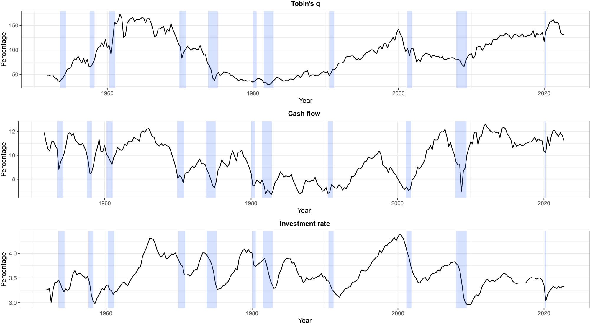
USA, 1951:Q4–2022:Q4. Time series plots of Tobin’s q, cash flow, and investment rate. Shaded areas indicate the NBER recession dates.
From Figure 1, it is possible to observe that the procyclical
During this period, the behavior of
To illustrate these points further, we provide a more detailed analysis for six different sub-periods – which, broadly speaking, try to capture the effects across different decades.
Table 1 presents some relevant descriptive statistics for the
Descriptive statistics for Tobin’s q, cash flow, and investment rate
| Period | Mean | Median | Standard deviation | Skewness | Kurtosis |
|---|---|---|---|---|---|
|
Tobin’s q:
|
|||||
| 1951:Q4–1969:Q4 | 111.29 | 120.91 | 43.26 |
|
|
| 1970:Q1–1979:Q4 | 66.66 | 54.14 | 27.22 | 0.35 |
|
| 1980:Q1–1989:Q4 | 42.52 | 41.40 | 7.40 | 0.22 |
|
| 1990:Q1–1999:Q4 | 88.80 | 87.61 | 21.04 | 0.001 |
|
| 2000:Q1–2009:Q4 | 89.64 | 86.25 | 15.36 | 1.71 | 3.10 |
| 2010:Q1–2022:Q4 | 126.66 | 129.24 | 17.12 |
|
0.25 |
|
Cash flow:
|
|||||
| 1951:Q4–1969:Q4 | 10.71 | 10.81 | 0.87 |
|
|
| 1970:Q1–1979:Q4 | 9.04 | 9.11 | 0.80 |
|
|
| 1980:Q1–1989:Q4 | 7.65 | 7.73 | 0.53 |
|
|
| 1990:Q1–1999:Q4 | 8.47 | 8.52 | 1.07 | 0.06 |
|
| 2000:Q1–2009:Q4 | 9.52 | 9.37 | 1.60 |
|
|
| 2010:Q1–2022:Q4 | 11.48 | 11.53 | 0.56 |
|
|
|
Investment rate:
|
|||||
| 1951:Q4–1969:Q4 | 3.55 | 3.45 | 0.35 | 0.56 |
|
| 1970:Q1–1979:Q4 | 3.70 | 3.68 | 0.25 |
|
|
| 1980:Q1–1989:Q4 | 3.64 | 3.61 | 0.19 | 0.07 |
|
| 1990:Q1–1999:Q4 | 3.65 | 3.61 | 0.38 | 0.32 |
|
| 2000:Q1–2009:Q4 | 3.66 | 3.64 | 0.35 | 0.13 | 0.10 |
| 2010:Q1–2022:Q4 | 3.38 | 3.40 | 0.15 |
|
0.29 |
Note: The time series
Importantly, Table 1 also shows that there have been considerable changes in the volatility of the three series across decades. The respective standard deviations show important evidence of time variation, especially the ones for
Figures 2 and 3 show the scatter plots between
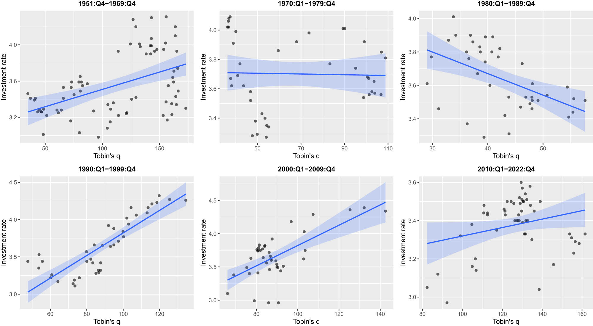
USA, 1951:Q4–2022:Q4. Scatter plots between investment rate and Tobin’s q for different sub-periods. Straight lines show ordinary least squares (OLS) regression lines, assuming that all values of cash flow are fixed at zero. Shaded areas indicate 95% confidence level intervals of the regression lines.
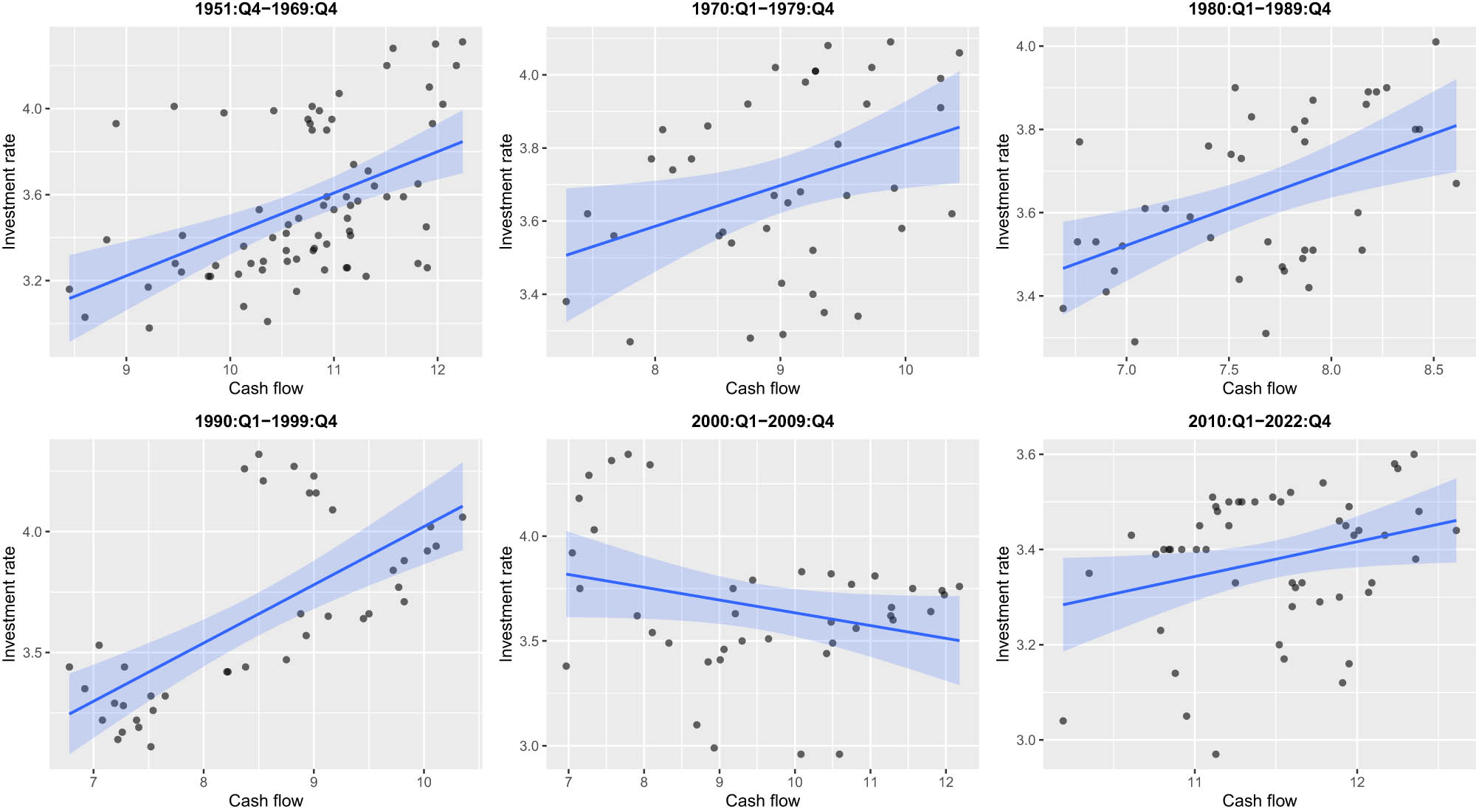
USA, 1951:Q1–2022:Q4. Scatter plots between investment rate and cash flow for different sub-periods. Straight lines show OLS regression lines, assuming that all values of Tobin’s q are fixed at zero. Shaded areas indicate 95% confidence level intervals of the regression lines.
Finally, we summarize the response of
Investment rate equation,
| Period | Intercept: | Coefficient on Tobin’s q: | Coefficient on cash flow: |
|---|---|---|---|
|
|
|
|
|
| 1951:Q4–1969:Q4 | 1.548** | 0.003** | 0.155** |
| (0.587) | (0.001) | (0.057) | |
| 1970:Q1–1979:Q4 | 2.551** | 0.001 | 0.121* |
| (0.497) | (0.002) | (0.051) | |
| 1980:Q1–1989:Q4 | 2.903** |
|
0.161** |
| (0.493) | (0.003) | (0.054) | |
| 1990:Q1–1999:Q4 | 1.872** | 0.012** | 0.079 |
| (0.361) | (0.003) | (0.041) | |
| 2000:Q1–2009:Q4 | 2.359** | 0.015** |
|
| (0.389) | (0.002) | (0.030) | |
| 2010:Q1–2022:Q4 | 2.168** | 0.002 | 0.079* |
| (0.563) | (0.002) | (0.037) |
Notes: We report the OLS regression coefficients of the investment rate as a function of Tobin’s q and cash flow for different sub-periods, where
The stylized facts presented in this section suggest that the dynamics of
Motivated by this evidence, we use a TVP-VAR-SV model to formally study the interactions between the three variables and, most importantly, to capture the possible structural time-varying effects of both
4 Empirical Model
A reduced-form TVP-VAR-SV model of order
where
We can rewrite equation (1) as follows:
where
Hence, as in Primiceri (2005), the model depicted by equation (2) incorporates two types of parameter instability: TVPs via
The dynamics of the model’s TVPs are specified as follows:
where
Let us now define
where
We rely on Markov chain Monte Carlo (MCMC) methods to estimate the TVP-VAR-SV model outlined earlier. First, we follow Primiceri (2005)’s sampling algorithm, but we modify the latter by incorporating the correction noted by Del Negro and Primiceri (2015). Second, we use the same prior distributions and initial states of the parameter distributions employed by Primiceri (2005).[7] Third, using the relevant MCMC algorithm, we collect 205,000 posterior samples and discard the first 5,000 draws to ensure the convergence of the chain. Fourth, as in Primiceri (2005), we use
5 Summary of Findings
Our baseline results reported in this section consider the following ordering of variables to generate the impulse response functions (IRFs):
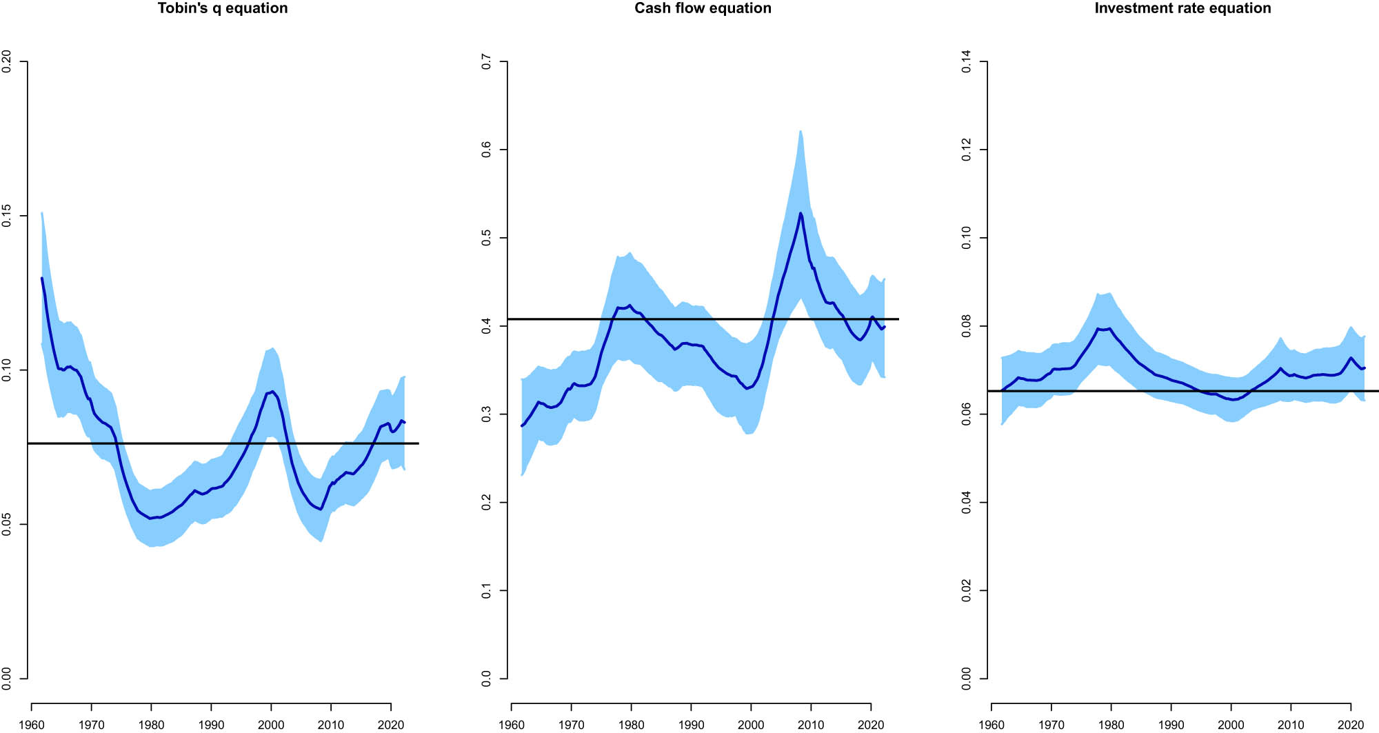
Posterior means of the standard deviations of residuals obtained from the TVP-VAR-SV model for the period 1961:Q4–2022:Q4. We report the time series plots of the means of the standard deviations of the residuals of Tobin’s q equation, cash flow equation, and investment rate equation in the TVP-VAR-SV model. Shaded areas show the 16th and 84th percentiles. Black horizontal lines show the means of the standard deviations of the residuals obtained from a standard VAR model (without TVP or SV) estimated via frequentist methods.
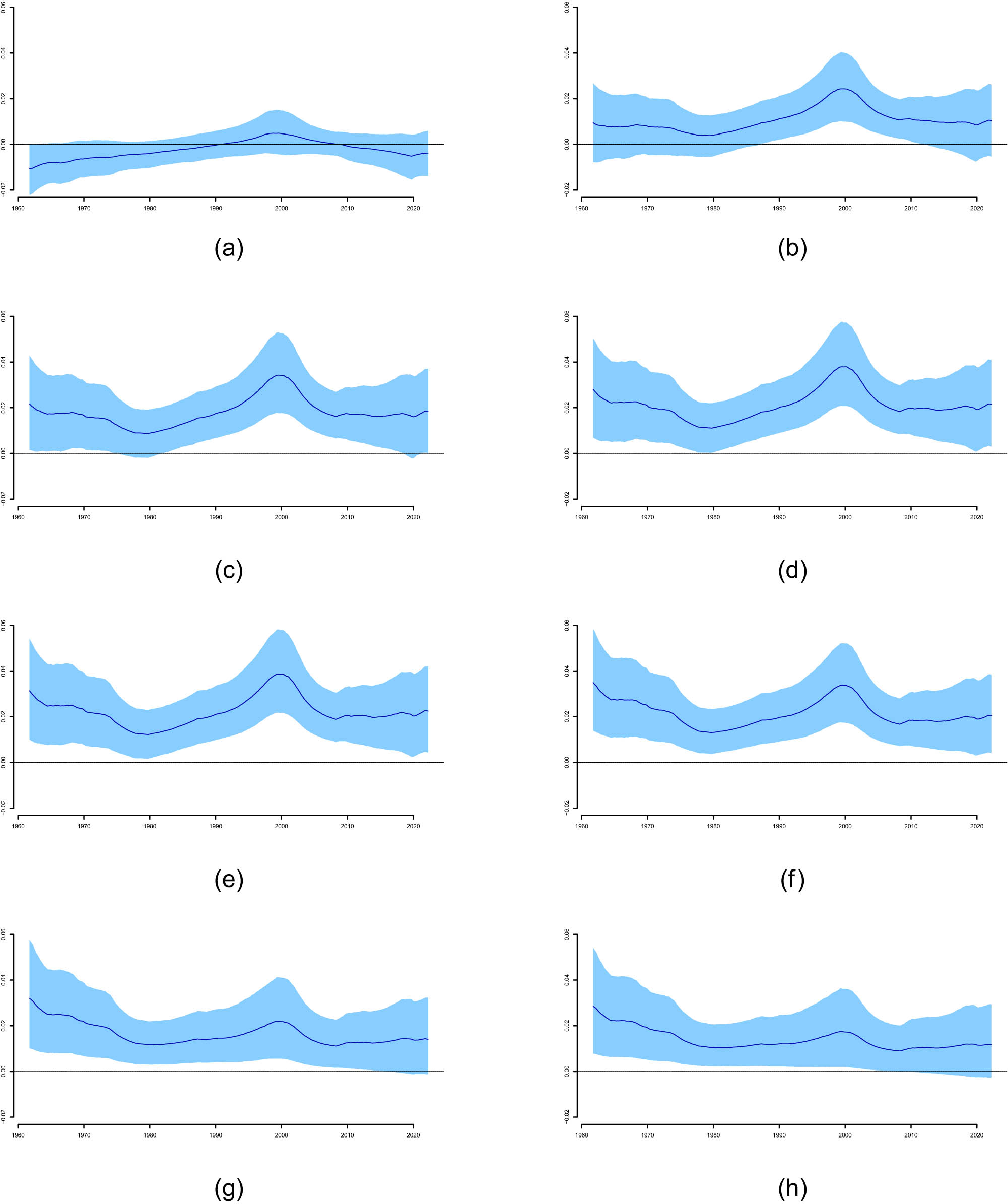
Time-varying response of investment rate to a shock in Tobin’s q at different quarters obtained from the TVP-VAR-SV model for the period 1961:Q4–2022:Q4. We report the time-varying median responses of the investment rate to a shock in Tobin’s q for different horizons. Shaded areas show the 16th and 84th percentiles: (a) within quarter (contemporaneous), (b) 1 quarter ahead, (c) 2 quarters ahead, (d) 3 quarters ahead, (e) 4 quarters ahead, (f) 8 quarters ahead, (g) 16 quarters ahead, and (h) 20 quarters ahead.
We begin by assessing the relevance of incorporating time-varying volatilities into the model by plotting the SVs aimed at capturing the heteroscedasticity of the shocks. Therefore, in Figure 4, we show the posterior mean together with the 16th and 84th percentiles of the time-varying standard deviation of the structural shocks. This is important to understand whether some variations in the dynamics in the model are associated with the variance–covariance matrix besides the TVPs in the model. We observe that the results indicate substantial time variation in the volatility of shocks. Specifically, Figure 4 shows that (i) the volatility of the shocks from the
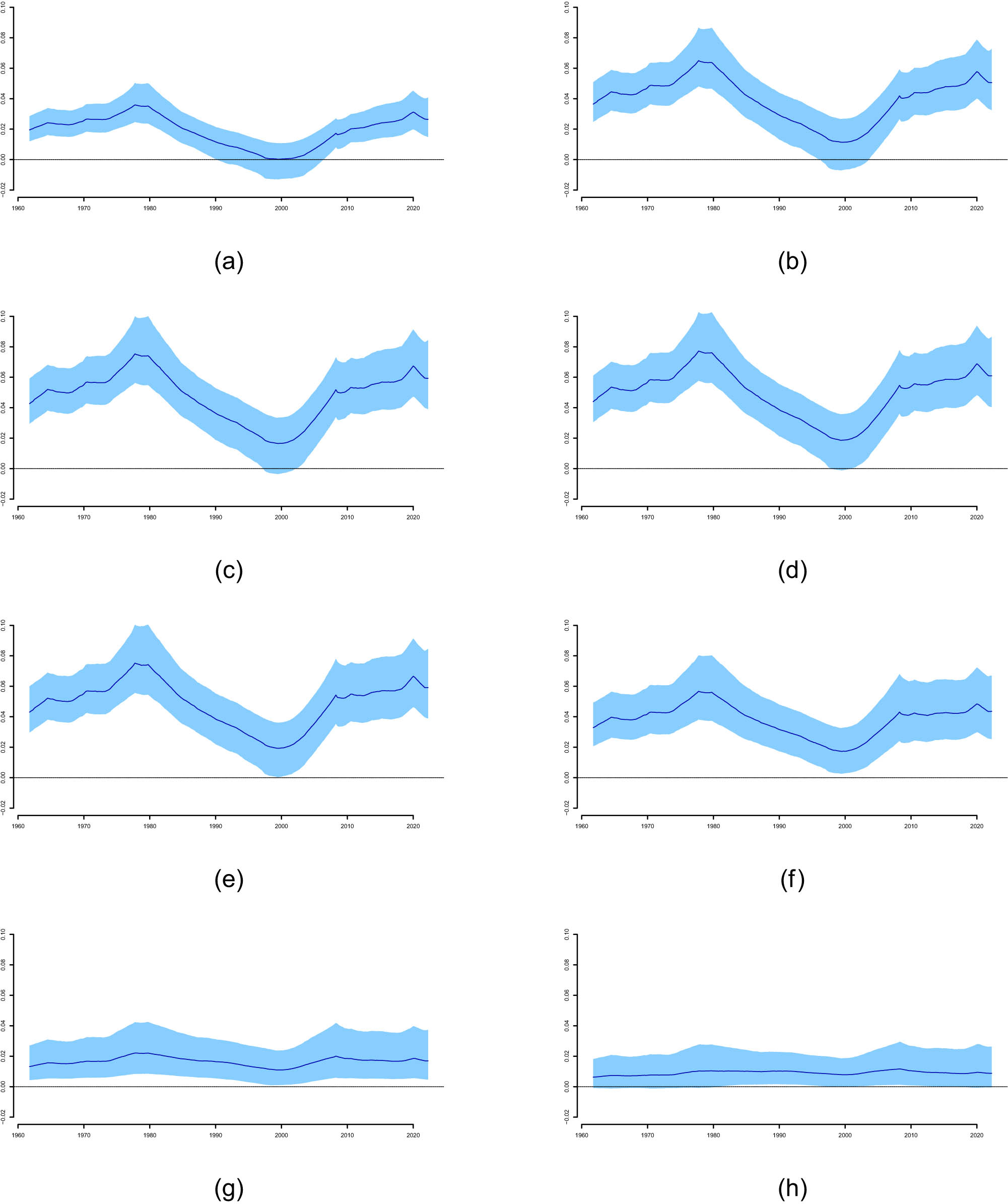
Time-varying response of investment rate to a shock in cash flow at different quarters obtained from the TVP-VAR-SV model for the period 1961:Q4–2022:Q4. We report the time-varying median responses of the investment rate to a shock in cash flow for different horizons. Shaded areas show the 16th and 84th percentiles: (a) within quarter (contemporaneous), (b) 1 quarter ahead, (c) 2 quarters ahead, (d) 3 quarters ahead, (e) 4 quarters ahead, (f) 8 quarters ahead, (g) 16 quarters ahead, and (h) 20 quarters ahead.
Since our main interest consists in studying the possible time-varying effects of both
Figure 5 shows that a positive shock in
Regarding the possible changing nature of the effects of
The results in Figure 6 show that most of the error bands do not enclose the zero line, thus indicating a strong positive response of
Nevertheless, it is also clear that the response of
The main results can be summarized as follows. First, we find robust evidence of time-varying sensitivities of
Second, in the short-run, the evolution of the time-varying response of
Our empirical results corroborate the effects discussed by Abel and Eberly (2012) at the theoretical level, who showed that if growth options for firms are important and the firms’ productivity level is assumed to be endogenous (i.e., if it is assumed to be a choice variable), then
6 Conclusions
What are the time-varying effects of the availability of external equity finance, approximated by Tobin’s q, and the availability of internal funds, approximated by cash flow, on the dynamics of aggregate investment? We answer this question for the post-World War II US economy by estimating a TVP-VAR-SV model via Bayesian methods.
We find new empirical evidence that contributes to our understanding of short-run fluctuations in investment. First, there is strong evidence showing that investment exhibits important time-varying sensitivities to both variables, thus indicating the existence of relevant structural changes in the dynamics of investment and its linkages to Tobin’s q and cash flow.
Second, the evolution of the time-varying sensitivity of investment to a shock to Tobin’s q decreased since the early 1960s through the early 1980s, increased since the early 1980s through the early 2000s, and it has decreased importantly again since then. By contrast, the time-varying sensitivity of investment to a shock to cash flow increased since the early 1960s through the early 1980s, decreased since the early 1980s through the early 2000s, and it has tended to increase importantly again since then. We find that these time-varying investment sensitivities are most strongly observed within a 2-year horizon, thus suggesting that these effects are mainly predominant in the short-run.
Hence, the short-run evolution of the time-varying response of investment to shocks to Tobin’s q is almost the mirror image to the short-run evolution of the time-varying response of investment to shocks to cash flow. These results indicate that although Tobin’s q and cash flow can be regarded as complementary sources of information for aggregate investment because both variables influence simultaneously firms’ investment decisions, the relative importance of each variable for investment fluctuations has changed considerably over time. This implies that both variables should also be regarded as alternative to each other in order to understand firms’ investment at the aggregate level in the short-run.
Future studies could fruitfully explore this finding further as follows. First, novel theoretical elements are needed to better understand the mechanisms that ultimately generate this phenomenon – by establishing a direct link between the relevant technological upgrades that may influence firms’ investment decisions to rely more heavily on cash flow or Tobin’s q during specific periods. Second, novel empirical research is also needed to identify the specific structural changes that shape the behavior of the TVPs and volatilities. This is work that remains to be done.
Acknowledgements
I am deeply grateful to two anonymous referees for valuable comments and suggestions, which have significantly improved the final version of the article. I have also benefited from comments by Bowen Fu and Mengheng Li. Any remaining errors are the responsibility of the author.
-
Funding information: This project was supported by the University Research Committee (URC) at the University of Utah. Its contents are solely the responsibility of the author and do not necessarily represent the official views of the URC, the Vice President for Research Office, or the University of Utah.
-
Author contributions: The author confirms the sole responsibility for the conception of the study, presented results and manuscript preparation.
-
Conflict of interest: The author states no conflict of interest.
-
Article note: As part of the open assessment, reviews and the original submission are available as supplementary files on our website.
-
Data availability statement: The dataset used in this article is available from the author on request.
Appendix A Priors
In all the estimated TVP-VAR-SV models,
where
As in Primiceri (2005), we also use the first 10 years (40 observations with quarterly data) to calibrate the prior distributions, so that
B Summary of the MCMC Sampling Algorithm
We implement the MCMC sampling algorithm of Primiceri (2005) considering the correction noted by Del Negro and Primiceri (2015), which corresponds to “Algorithm 2” in the latter. Compared to Primiceri (2005)’s original algorithm, Del Negro and Primiceri (2015) proposed that the sampling of the stochastic volatilities should be carried out after the sampling of the states of the mixture of normals components approximation to a
Let us denote
Initialize
Draw
Draw
Draw
Draw
Draw
Draw
Draw
Go to Step 2.
C Impulse Responses for the Baseline Model for Specific Dates
Figure A1 shows the impulse responses following a shock to
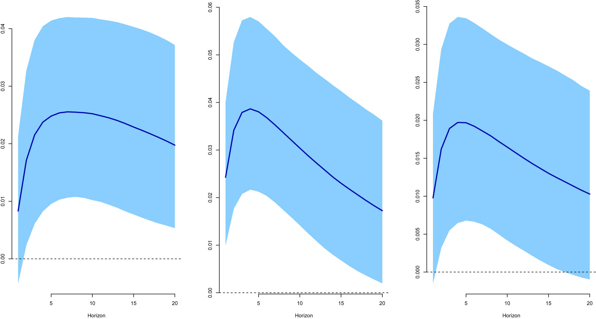
Response of investment rate to a shock in Tobin’s q for selected dates obtained from the TVP-VAR-SV model. We report the median responses of the investment rate to a shock in Tobin’s q in: 1969:Q4 (left panel), 2000:Q3 (middle panel), and 2014:Q3 (right panel). Shaded areas show the 16th and 84th percentiles.
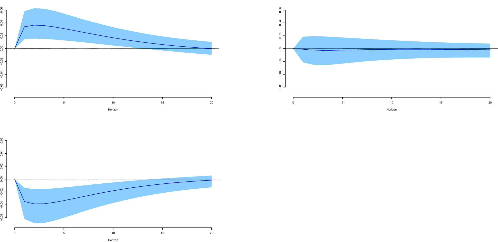
To further illustrate these effects, Figure A2 plots the differences between the impulse responses in 1969:Q4 and 2000:Q3, 1969:Q4 and 2014:Q3, and 2000:Q3 and 2014:Q3. Since the error bands do not enclose the zero line for the difference between the impulse response in 2000:Q3 and 2014:Q3, we can conclude that the impulse response is significantly stronger in 2000:Q3 than in 2014:Q3 (see the bottom-left panel in Figure A2).
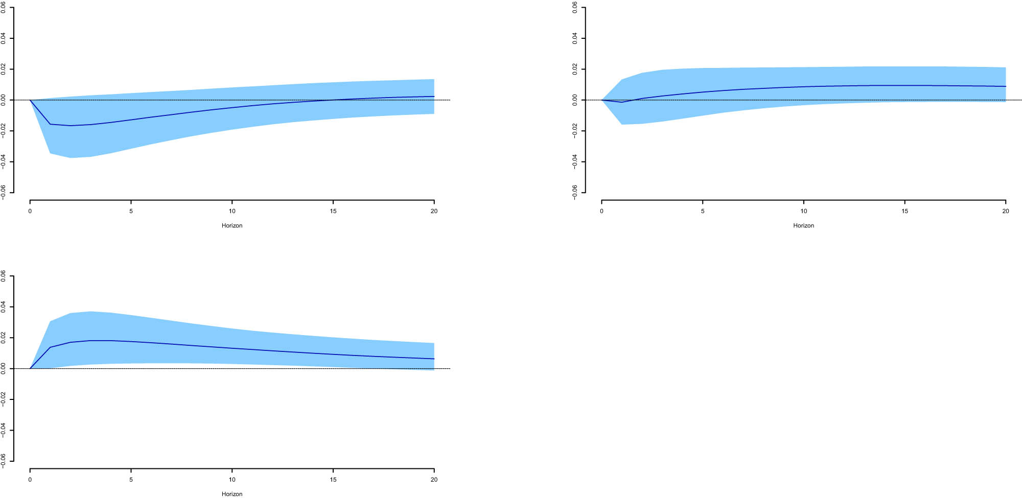
Differences in the response of investment rate to a shock in Tobin’s q for selected dates obtained from the TVP-VAR-SV model. We report the differences of the median responses of the investment rate to a shock in Tobin’s q between: 1969:Q4–2000:Q3 (top-left panel), 1969:Q4–2014:Q3 (top-right panel), and 2000:Q3–2014:Q3 (bottom-left panel). Shaded areas show the 16th and 84th percentiles.
The response of
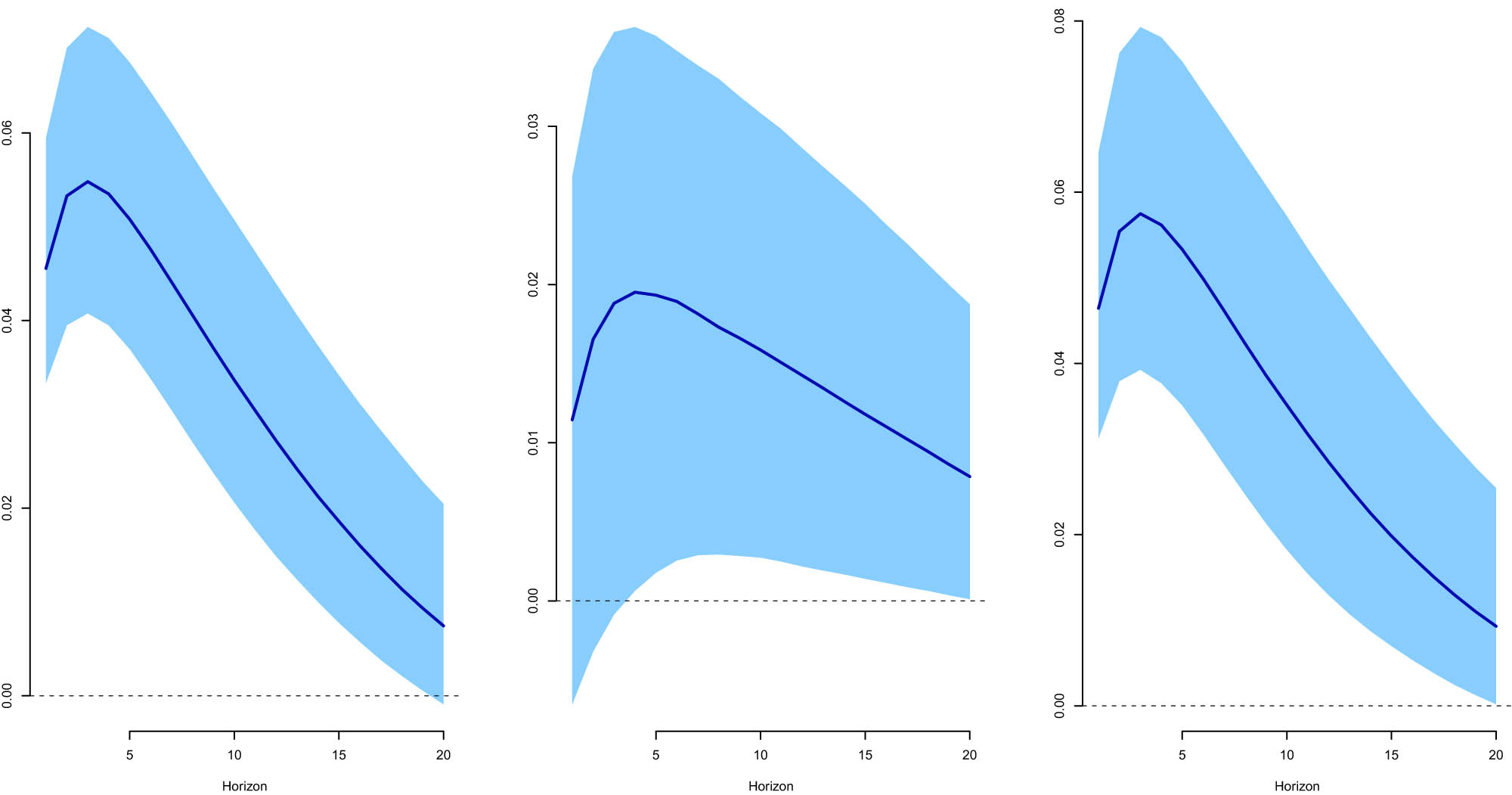
Response of investment rate to a shock in cash flow for selected dates obtained from the TVP-VAR-SV model. We report the median responses of the investment rate to a shock in cash flow in: 1969:Q4 (left panel), 2000:Q3 (middle panel), and 2014:Q3 (right panel). Shaded areas show the 16th and 84th percentiles.
Figure A4 plots the differences between the impulse responses in 1969:Q4 and 2000:Q3, 1969:Q4 and 2014:Q3, and 2000:Q3 and 2014:Q3. Considering the estimation uncertainty summarized by the error bands, it is possible to conclude that the impulse response is significantly stronger in 1969:Q4 than in 2000:Q3 (top-left panel in Figure A4) and significantly weaker in 2000:Q3 than in 2014:Q3 (bottom-left panel in Figure A4).
Differences in the response of investment rate to a shock in cash flow for selected dates obtained from the TVP-VAR-SV model. We report the differences of the median responses of the investment rate to a shock in cash flow between: 1969:Q4–2000:Q3 (top-left panel), 1969:Q4–2014:Q3 (top-right panel), and 2000:Q3–2014:Q3 (bottom-left panel). Shaded areas show the 16th and 84th percentiles.
References
Abel, A. B., & Eberly, J. C. (2011). How Q and cash flow affect investment without frictions: An analytic explanation. The Review of Economic Studies, 78(4), 1179–1200. https://doi.org/10.1093/restud/rdr006. Search in Google Scholar
Abel, A. B., & Eberly, J. C. (2012). Investment, valuation, and growth options. The Quarterly Journal of Finance, 2(1), 1250001. https://doi.org/10.1142/S2010139212500012. Search in Google Scholar
Antolin-Diaz, J., Drechsel, T., & Petrella, I. (2017). Tracking the slowdown in long-run GDP growth. The Review of Economics and Statistics, 99(2), 343–356. https://doi.org/10.1162/REST_a_00646. Search in Google Scholar
Ağca, Ş, & Mozumdar, A. (2008). The impact of capital market imperfections on investment-cash flow sensitivity. Journal of Banking Finance, 32(2), 207–216. https://doi.org/10.1016/j.jbankfin.2007.02.013. Search in Google Scholar
Brown, J. R., & Petersen, B. C. (2009). Why has the investment-cash flow sensitivity declined so sharply? Rising RD and equity market developments. Journal of Banking Finance, 33(5), 971–984. https://doi.org/10.1016/j.jbankfin.2008.10.009. Search in Google Scholar
Carter, C. K., & Kohn, R. (1994). On Gibbs sampling for state space models. Biometrika, 81(3), 541–553. https://doi.org/10.1093/biomet/81.3.541. Search in Google Scholar
Chen, H., & Chen, S. (2012). Investment-cash flow sensitivity cannot be a good measure of financial constraints: Evidence from the time series. Journal of Financial Economics, 103(2), 393–410. https://doi.org/10.1016/j.jfineco.2011.08.009. Search in Google Scholar
Del Negro, M., & Primiceri, G. E. (2015). Time-varying structural vector autoregressions and monetary policy: A corrigendum. The Review of Economic Studies, 82(4), 1342–1345. https://doi.org/10.1093/restud/rdv024. Search in Google Scholar
Gallegati, M., & Ramsey, J. B. (2013). Structural change and phase variation: A re-examination of the q-model using wavelet exploratory analysis. Structural Change and Economic Dynamics, 25(June), 60–73. https://doi.org/10.1016/j.strueco.2013.02.002. Search in Google Scholar
Gordon, R. J. (2015). Secular stagnation: A supply-side view. American Economic Review, 105(5), 54–59. https://doi.org/10.1257/aer.p20151102. Search in Google Scholar
Grabowski, H. G., & Mueller, D. C. (1972). Managerial and stockholder welfare models of firm expenditures. The Review Economics and Statistics, 54(1), 9–24. https://doi.org/10.2307/1927491. Search in Google Scholar
Grullon, G., Hund, J., & Weston, J. P. (2018). Concentrating on q and cash flow. Journal of Financial Intermediation, 33(January), 1–15. https://doi.org/10.1016/j.jfi.2017.10.001. Search in Google Scholar
Gugler, K., Mueller, D. C., & Yortoglu, B. B. (2004). Marginal q, Tobin’s q, cash flow, and investment. Southern Economic Journal, 70(3), 512–531. https://doi.org/10.2307/4135328. Search in Google Scholar
Gutiérrez, G., & Phillippon, T. (2017). Investment-less growth: An empirical investigation. Brookings Papers on Economic Activity, 48(2), 89–190. https://www.brookings.edu/wp-content/uploads/2018/02/gutierreztextfa17bpea.pdf. Search in Google Scholar
Haque, Q., Magnusson, L. M., & Tomioka, K. (2021). Empirical evidence on the dynamics of investment under Uncertainty in the U.S. Oxford Bulletin of Economics and Statistics, 83(5), 1193–1217. https://doi.org/10.1111/obes.12420. Search in Google Scholar
Kim, S., Shephard, N., & Chib, S. (1998). Stochastic volatility: Likelihood inference and comparison with ARCH models. The Review of Economic Studies, 65(3), 361–393. https://doi.org/10.1111/1467-937X.00050. Search in Google Scholar
Lettau, M., & Ludvigson, S. (2002). Time-varying risk premia and the cost of capital: An alternative implication of the Q theory of investment. Journal of Monetary Economics, 49(1), 31–66. https://doi.org/10.1016/S0304-3932(01)00097-6. Search in Google Scholar
Li, M., & Mendieta-Muñoz, I. (2020). Are long-run output growth rates falling? Metroeconomica, 71(1), 204–234. https://doi.org/10.1111/meca.12275. Search in Google Scholar
Lewellen, J., & Lewellen, K. (2002). Investment and cash flow: New evidence. Journal of Financial and Quantitative Analysis, 51(4), 1135–1164. https://doi.org/10.1017/S002210901600065X. Search in Google Scholar
Mclean, R. D., & Zhao, M. (2014). The business cycle, investor sentiment, and costly external finance. Journal of Finance, 69(3), 1377–1409. https://doi.org/10.1111/jofi.12047. Search in Google Scholar
Mendieta-Muñoz, I., & Sündal, D. (2022). Business cycles, financial conditions, and nonlinearities. Metroeconomica, 73(2), 343–383. https://doi.org/10.1111/meca.12363. Search in Google Scholar
Primiceri, G. E. (2005). Time varying structural vector autoregressions and monetary policy. The Review of Economic Studies, 72(3), 821–852. https://doi.org/10.1111/j.1467-937X.2005.00353.x. Search in Google Scholar
Stiglitz, J. E., & Weiss, A. (1981). Credit rationing in markets with imperfect information. American Economic Review, 71(3), 393–410. https://www.jstor.org/stable/1802787. Search in Google Scholar
Tobin, J. (1969). A general equilibrium approach to monetary theory. Journal of Money, Credit and Banking, 1(1), 15–29. https://doi.org/10.2307/1991374. Search in Google Scholar
Verona, F. (2020). Investment, Tobin’s Q, and cash flow across time and frequencies. Oxford Bulletin of Economics and Statistics, 82(2), 331–346. https://doi.org/10.1111/obes.12321. Search in Google Scholar
Welch, I., & Goyal, A. (2008). A comprehensive look at the empirical performance of equity premium prediction. The Review of Financial Studies, 21(4), 1455–1508. https://doi.org/10.1093/rfs/hhm014. Search in Google Scholar
© 2024 the author(s), published by De Gruyter
This work is licensed under the Creative Commons Attribution 4.0 International License.
Articles in the same Issue
- Regular Articles
- Political Turnover and Public Health Provision in Brazilian Municipalities
- Examining the Effects of Trade Liberalisation Using a Gravity Model Approach
- Operating Efficiency in the Capital-Intensive Semiconductor Industry: A Nonparametric Frontier Approach
- Does Health Insurance Boost Subjective Well-being? Examining the Link in China through a National Survey
- An Intelligent Approach for Predicting Stock Market Movements in Emerging Markets Using Optimized Technical Indicators and Neural Networks
- Analysis of the Effect of Digital Financial Inclusion in Promoting Inclusive Growth: Mechanism and Statistical Verification
- Effective Tax Rates and Firm Size under Turnover Tax: Evidence from a Natural Experiment on SMEs
- Re-investigating the Impact of Economic Growth, Energy Consumption, Financial Development, Institutional Quality, and Globalization on Environmental Degradation in OECD Countries
- A Compliance Return Method to Evaluate Different Approaches to Implementing Regulations: The Example of Food Hygiene Standards
- Panel Technical Efficiency of Korean Companies in the Energy Sector based on Digital Capabilities
- Time-varying Investment Dynamics in the USA
- Preferences, Institutions, and Policy Makers: The Case of the New Institutionalization of Science, Technology, and Innovation Governance in Colombia
- The Impact of Geographic Factors on Credit Risk: A Study of Chinese Commercial Banks
- The Heterogeneous Effect and Transmission Paths of Air Pollution on Housing Prices: Evidence from 30 Large- and Medium-Sized Cities in China
- Analysis of Demographic Variables Affecting Digital Citizenship in Turkey
- Green Finance, Environmental Regulations, and Green Technologies in China: Implications for Achieving Green Economic Recovery
- Coupled and Coordinated Development of Economic Growth and Green Sustainability in a Manufacturing Enterprise under the Context of Dual Carbon Goals: Carbon Peaking and Carbon Neutrality
- Revealing the New Nexus in Urban Unemployment Dynamics: The Relationship between Institutional Variables and Long-Term Unemployment in Colombia
- The Roles of the Terms of Trade and the Real Exchange Rate in the Current Account Balance
- Cleaner Production: Analysis of the Role and Path of Green Finance in Controlling Agricultural Nonpoint Source Pollution
- The Research on the Impact of Regional Trade Network Relationships on Value Chain Resilience in China’s Service Industry
- Social Support and Suicidal Ideation among Children of Cross-Border Married Couples
- Asymmetrical Monetary Relations and Involuntary Unemployment in a General Equilibrium Model
- Job Crafting among Airport Security: The Role of Organizational Support, Work Engagement and Social Courage
- Does the Adjustment of Industrial Structure Restrain the Income Gap between Urban and Rural Areas
- Optimizing Emergency Logistics Centre Locations: A Multi-Objective Robust Model
- Geopolitical Risks and Stock Market Volatility in the SAARC Region
- Trade Globalization, Overseas Investment, and Tax Revenue Growth in Sub-Saharan Africa
- Can Government Expenditure Improve the Efficiency of Institutional Elderly-Care Service? – Take Wuhan as an Example
- Media Tone and Earnings Management before the Earnings Announcement: Evidence from China
- Review Articles
- Economic Growth in the Age of Ubiquitous Threats: How Global Risks are Reshaping Growth Theory
- Efficiency Measurement in Healthcare: The Foundations, Variables, and Models – A Narrative Literature Review
- Rethinking the Theoretical Foundation of Economics I: The Multilevel Paradigm
- Financial Literacy as Part of Empowerment Education for Later Life: A Spectrum of Perspectives, Challenges and Implications for Individuals, Educators and Policymakers in the Modern Digital Economy
- Special Issue: Economic Implications of Management and Entrepreneurship - Part II
- Ethnic Entrepreneurship: A Qualitative Study on Entrepreneurial Tendency of Meskhetian Turks Living in the USA in the Context of the Interactive Model
- Bridging Brand Parity with Insights Regarding Consumer Behavior
- The Effect of Green Human Resources Management Practices on Corporate Sustainability from the Perspective of Employees
- Special Issue: Shapes of Performance Evaluation in Economics and Management Decision - Part II
- High-Quality Development of Sports Competition Performance Industry in Chengdu-Chongqing Region Based on Performance Evaluation Theory
- Analysis of Multi-Factor Dynamic Coupling and Government Intervention Level for Urbanization in China: Evidence from the Yangtze River Economic Belt
- The Impact of Environmental Regulation on Technological Innovation of Enterprises: Based on Empirical Evidences of the Implementation of Pollution Charges in China
- Environmental Social Responsibility, Local Environmental Protection Strategy, and Corporate Financial Performance – Empirical Evidence from Heavy Pollution Industry
- The Relationship Between Stock Performance and Money Supply Based on VAR Model in the Context of E-commerce
- A Novel Approach for the Assessment of Logistics Performance Index of EU Countries
- The Decision Behaviour Evaluation of Interrelationships among Personality, Transformational Leadership, Leadership Self-Efficacy, and Commitment for E-Commerce Administrative Managers
- Role of Cultural Factors on Entrepreneurship Across the Diverse Economic Stages: Insights from GEM and GLOBE Data
- Performance Evaluation of Economic Relocation Effect for Environmental Non-Governmental Organizations: Evidence from China
- Functional Analysis of English Carriers and Related Resources of Cultural Communication in Internet Media
- The Influences of Multi-Level Environmental Regulations on Firm Performance in China
- Exploring the Ethnic Cultural Integration Path of Immigrant Communities Based on Ethnic Inter-Embedding
- Analysis of a New Model of Economic Growth in Renewable Energy for Green Computing
- An Empirical Examination of Aging’s Ramifications on Large-scale Agriculture: China’s Perspective
- The Impact of Firm Digital Transformation on Environmental, Social, and Governance Performance: Evidence from China
- Accounting Comparability and Labor Productivity: Evidence from China’s A-Share Listed Firms
- An Empirical Study on the Impact of Tariff Reduction on China’s Textile Industry under the Background of RCEP
- Top Executives’ Overseas Background on Corporate Green Innovation Output: The Mediating Role of Risk Preference
- Neutrosophic Inventory Management: A Cost-Effective Approach
- Mechanism Analysis and Response of Digital Financial Inclusion to Labor Economy based on ANN and Contribution Analysis
- Asset Pricing and Portfolio Investment Management Using Machine Learning: Research Trend Analysis Using Scientometrics
- User-centric Smart City Services for People with Disabilities and the Elderly: A UN SDG Framework Approach
- Research on the Problems and Institutional Optimization Strategies of Rural Collective Economic Organization Governance
- The Impact of the Global Minimum Tax Reform on China and Its Countermeasures
- Sustainable Development of Low-Carbon Supply Chain Economy based on the Internet of Things and Environmental Responsibility
- Measurement of Higher Education Competitiveness Level and Regional Disparities in China from the Perspective of Sustainable Development
- Payment Clearing and Regional Economy Development Based on Panel Data of Sichuan Province
- Coordinated Regional Economic Development: A Study of the Relationship Between Regional Policies and Business Performance
- A Novel Perspective on Prioritizing Investment Projects under Future Uncertainty: Integrating Robustness Analysis with the Net Present Value Model
- Research on Measurement of Manufacturing Industry Chain Resilience Based on Index Contribution Model Driven by Digital Economy
- Special Issue: AEEFI 2023
- Portfolio Allocation, Risk Aversion, and Digital Literacy Among the European Elderly
- Exploring the Heterogeneous Impact of Trade Agreements on Trade: Depth Matters
- Import, Productivity, and Export Performances
- Government Expenditure, Education, and Productivity in the European Union: Effects on Economic Growth
- Replication Study
- Carbon Taxes and CO2 Emissions: A Replication of Andersson (American Economic Journal: Economic Policy, 2019)