A numerical study of anomalous electro-diffusion cells in cable sense with a non-singular kernel
-
Azhar Iqbal
 and
Tayyaba Akram
and
Tayyaba Akram

Abstract
The time-fractional cable model is solved using an extended cubic B-spline (ECBS) collocation strategy. The B-spline function was used for space partitioning, while the Caputo-Fabrizio (CF) was used for temporal discretization. The finite difference technique was used to discretize the CF operator. For the first time in cable modeling, the CF operator has been used. In terms of time, the convergence of order
1 Introduction
Anomalous diffusion in cells has been observed in several research experiments, and this anomalous diffusion is primarily exhibited by fractional derivatives. Brownian motion can be used to explain the process of signal transmission to the insides of cells. As a consequence of the irregularity, the diffusion in the cells can become aberrant. The voltage transmission in axons is affected in this situation [1]. The fractional diffusion model has caught the interest of many academicians in recent years because of its numerous applications in various areas. The special case of time-fractional cable model [2] is one of these models that we will look at in this article.
with initial and boundary value conditions, respectively,
where
where
If
The CF derivative has added a new dimension to the study of fractional differential equations (FDEs). The Caputo, Riemann-Liouville, and other singular kernel operators have kernels for power law that have limitations in representing physical situations [4]. It is produced using the exponential function and regular derivative convolution and it retains the same intrinsic inspirational qualities of heterogeneity and configuration for many scales as the Caputo and Riemann-Liouville fractional derivatives [5,6, 7,8]. This derivative has already been mentioned in a number of articles, such as fractional Maxwell fluid [9], fluid flows [10], diffusive transport system [6], non-linear Fisher’s diffusion equation [11], and electric circuits [5]. To explain the electrotonic characteristics of spiny neural dendrites, Henry et al. [12] presented cable equations with fractional order temporal operators. The anomalous electrodiffusion can be alternatively modeled by a fractal-fractional model in [13,14]. He’s fractional derivative for the evolution equation has been adopted by Wang and Yao [15].
The time-fractional cable model is equivalent to the classic cable equation other than that the order of derivative is fractional with regard to time. Many fractional models have no analytical solutions due to the non-locality of fractional derivatives. Hence, numerical solutions to fractional differential model are important in terms of both science and practical application. As a result, several investigators have recently taken fractional differential models as a challenge and discovered numerical solutions to such problems. Two implicit compact difference techniques for solving fractional cable model were developed by Hu and Zhang [16]. Yu and Jiang [17] studied time-fractional cable model using fourth-order compact difference method. The local discontinuous Galerkin technique has been developed by Zheng and Zhao [18]. Yang et al. [19] proposed a temporal-spacial spectral-tau technique for solving fractional cable and its inverse model. Liu et al. [20,21] solved the fractional cable equations via finite element approximations and Grünwald difference approximations. Zhu et al. [22] presented the Galerkin finite element and convolution quadrature methods for the solution of fractional cable equation. Various researchers have worked on the solution of the FDEs by using numerical technique based on spline function [23,24, 25,26]. Li [27] has studied the Wavelet collocation approach based on B-spline functions for solving the FDEs. B splines helped to resolve the unknowns in the equation. It was shown that the B-spline finite element is useful for the numerical solutions of FDE, particularly when continuity of the solutions was essential. Saad et al. [28] used a Atangana-Baleanu fractional derivative with spectral collocation methods to approximate the solution of the fractional Fisher’s type equations. The results indicate that the proposed methodology is a simple and effective tool for studying nonlinear equations with local and non-local singular kernels. Akram et al. [29,30] investigated time fractional cable equation and sub-diffusion equation using B-spline methods, Riemann-Liouville, and Caputo derivatives. The stability and convergence of the proposed methods have also been examined. Moshtaghi and Saadatmandi [31] developed the numerical technique for time fractional cable problem using Sinc-Bernoulli and Riemann-Liouville methods. A Galerkin method with spline function for solving time fractional diffusion equation has been proposed by Pezza and Pitolli [32]. Tabriz et al. [33] developed the operational matrix method based on Caputo derivative to solve fractional optimal control problem.
Despite the fact that B-spline has been used to solve fractional partial differential equations in several articles, we are not aware of any research that has used B-spline to solve time-fractional cable model equations. The B-spline function has very suitable properties for designing such convex hull and continuity properties [34]. Thus, the main objective of this research is to use the extended cubic B-spline (ECBS) to develop the collocation approach for the time-fractional cable model. The strategy’s main feature is that it converts such problems into algebraic system of equations that can be used in programming. The following is the organization of this research article: Section 2 presents the extended cubic B-spline (ECBS) functions and time approximation. The ECBS collocation method is presented in Section 3. The stability analysis is proved in Section 4. Sections 5 and 6 discuss the numerical experiment as well as the conclusion.
2 Preliminaries
2.1 ECBS functions
Assume that
where
The ECBS functions (4) and equation (5) yield the equations as follows:
2.2 Difference method for the CF
In this section, we look at using CF to discretize fractional time derivatives. Assume that
The discretized formulation [23] is as follows:
The truncation error is [23] as follows:
where
3 Derivation of the ECBS
To develop the numerical strategy for solving the cable model, we use the finite difference method, the CF, and the EBSM in this section. By plugging equations (9) and (4) in equation (1), we obtain
The nonlinear term is linearized by Taylor’s series expansion as follows:
which implies that
Using equation (12) in (11), we obtain
The aforementioned equation can be written in another form as:
where
The aforementioned system of equations have the order
Hence, we have the
3.1 Algorithm
Describe the model.
Discretize the modeled problem using the CF operator in time direction.
Linearize the nonlinear terms.
Discretize the problem using ECBS formulation in space direction.
Apply the two boundary conditions.
Resulting system of order
Solve the aforementioned system using Mathematica.
4 Stability and convergence analysis
The stability concept is linked to computation approach errors that do not increase as the procedure continues. The Von Neumann stability technique also known as Fourier stability is a method utilized to analyze the stability of difference techniques. Here, we will use the Von Neumann technique to investigate the stability of the proposed method. Assume that
To linearize the non-linear term in (11), we use
The aforementioned equation becomes
By inserting equation (14) in equation (15), we obtain the following error equation:
Consider the error solution for the B-spline can be written in one Fourier mode as
where
where
Taking the part that is identical on both sides and dividing it by
where
Proposition 4.1
Consider
Proof
Here, we use mathematical induction to validate this result. The following equation can be obtained when we choose
Suppose that
Thus,
Theorem 1
Let
where
Proof
The non-linear term in (11) can be linearized as
For
Taking inner product of the aforementioned equation with
For
which implies that
where
Using
which implies that
By dividing throughout with
By Gronwall’s inequality, we obtain
5 Numerical results
In this section, we incorporate the simulation findings of given problem by using the provided scheme. The numerical findings are used to test the claimed method validity and efficiency. The main goal of these examples is to examine the degree of convergence of the estimated results for
Example 1
with
and
The exact solution of the problem is:
By taking
|
|
|
|||
|---|---|---|---|---|
|
|
Proposed method
|
Proposed method
|
Order | |
| 1/5 |
|
|
|
|
| 1/10 |
|
|
|
1.02126 |
| 1/20 |
|
|
|
1.08926 |
| 1/40 |
|
|
|
1.01856 |
|
|
|
|||
|---|---|---|---|---|
|
|
Proposed method
|
Proposed method
|
Order | |
| 1/5 |
|
|
|
|
| 1/10 |
|
|
|
1.04435 |
| 1/20 |
|
|
|
1.05722 |
| 1/40 |
|
|
|
1.04936 |
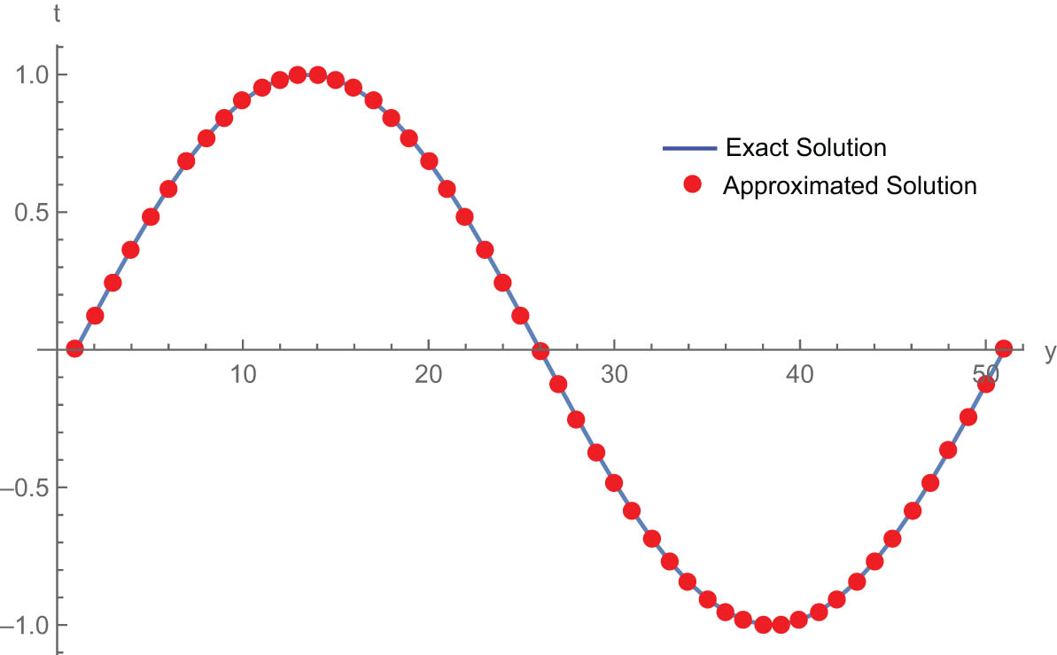
Exact and approximated solution of Example 1 for value of
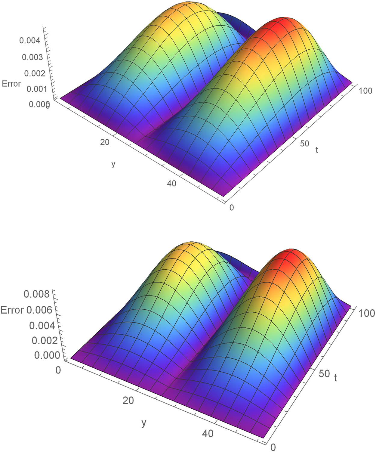
Space-time absolute error plot for value of
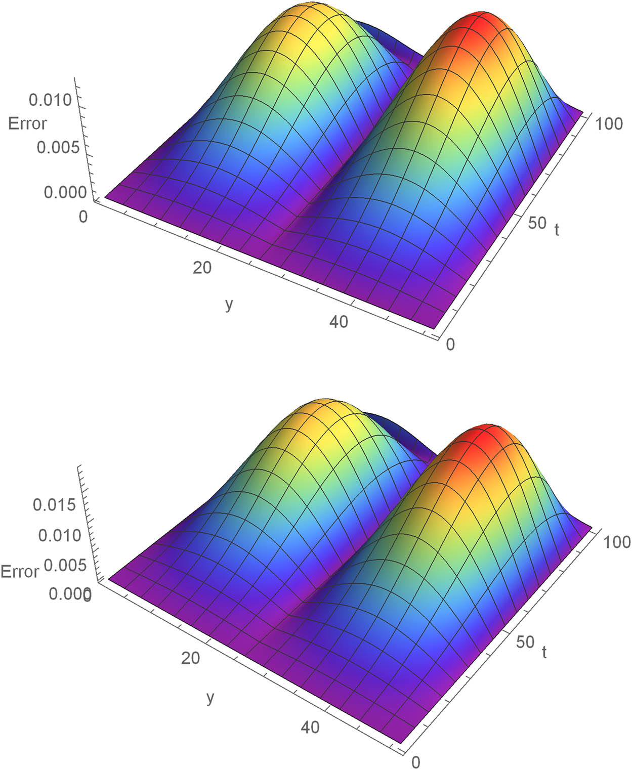
Space-time absolute error plot for value of
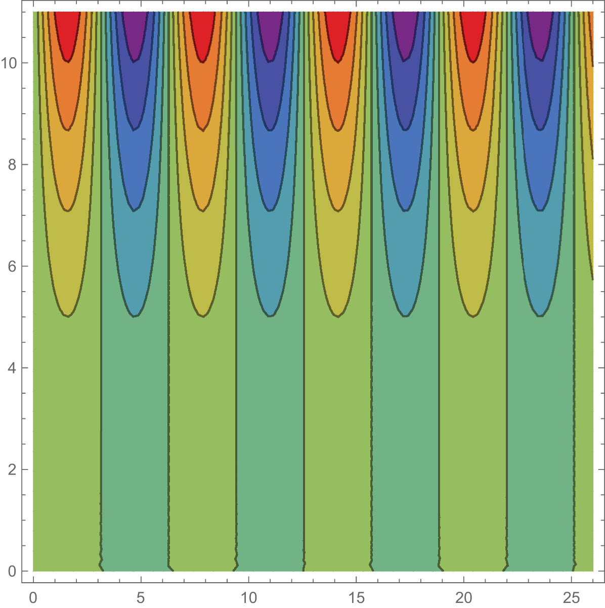
Contour plot for value of
Absolute errors for different
|
|
|
|
|
|
|---|---|---|---|---|
| 0.1 | 0.000505826 | 0.00093832 | 0.00137872 | 0.00183893 |
| 0.2 | 0.000839704 | 0.00160334 | 0.00239615 | 0.00340647 |
| 0.3 | 0.000852242 | 0.00161478 | 0.00240241 | 0.00340672 |
| 0.4 | 0.000587011 | 0.00103535 | 0.00145486 | 0.00185383 |
| 0.5 | 0.000342879 | 0.00053744 | 0.00058313 | 0.00040270 |
| 0.6 | 0.000419648 | 0.00080647 | 0.00090600 | 0.00103866 |
| 0.7 | 0.000677912 | 0.00148961 | 0.00193893 | 0.00299914 |
| 0.8 | 0.000658044 | 0.00147090 | 0.00192816 | 0.00299863 |
| 0.9 | 0.000319919 | 0.00068692 | 0.00081109 | 0.00101909 |
6 Conclusion
This study describes an ECBS collocation strategy for solving the time-fractional cable model. For space partitioning, the ECBS was used, whereas for temporal discretization, the CF was applied. The CF operator was discretized using the finite difference technique. The CF operator has been utilized for the first time in the cable model. The technique has order
Acknowledgments
The authors would like to thank Prince Mohammad Bin Fahd Center for Futuristic Studies and World Futures Studies Federation, Saudi Arabia, for their financial assistance.
-
Author contributions: All authors contributed equally. All authors read and approved the final manuscript.
-
Conflict of interest: The authors state no conflict of interest.
References
[1] E. J. López-Sáchez, J. M. Romero, and Y. Martínez, Fractional cable equation for general geometry: A model of axons with swellings and anomalous diffusion, Phys. Rev. E. 96 (2017), 032411, https://doi.org/10.1103/PhysRevE.96.032411. Search in Google Scholar PubMed
[2] Z. Wang, On Caputo type cable equation: Analysis and computation, Comput. Model. Eng. Sci. 123 (2020), 353–376, https://doi.org/10.32604/cmes.2020.08776. Search in Google Scholar
[3] J. Losada and J. J. Nieto, Properties of a new fractional derivative without singular Kernel, Prog. Fract. Differ. Appl. 1 (2015), no. 2, 87–92, https://doi.org/10.12785/pfda/010202. Search in Google Scholar
[4] M. Caputo and M. Fabrizio, A new definition of fractional derivative without singular Kernel, Prog. Fract. Differ. Appl. 1 (2015), no. 3, 73–85, https://doi.org/10.12785/pfda/010201. Search in Google Scholar
[5] A. Atangana and B. S. T. Alkahtani, Extension of the resistance inductance, capacitance electrical circuit of fractional derivative without singular kernel, Adv. Mech. Eng. 7 (2015), no. 6, 1–6, https://doi.org/10.1177/1687814015591937. Search in Google Scholar
[6] J. F. Gómez-Aguilar, M. G. Lopez-Lopez, V. M. Alvarado-Martınez, J. Reyes-Reyes, and M. Adam-Medina, Modeling diffusive transport with a fractional derivative without singular kernel, Phys. A 447 (2016), 467–481, https://doi.org/10.1016/j.physa.2015.12.066. Search in Google Scholar
[7] S. Djennadi, N. Shawagfeh, M. S. Osman, J. F. Gómez-Aguilar, and O. A. Abu Arqub, The Tikhonov regularization method for the inverse source problem of time fractional heat equation in the view of ABC-fractional technique, Phys. Scr. 96 (2021), 094006, https://doi.org/10.1088/1402-4896/ac0867. Search in Google Scholar
[8] S. Momani, B. Maayah, and O. AbuArqub, The reproducing kernel algorithm for numerical solution of Van der Poldamping model in view of the Atangana-Baleanu fractional approach, Fractals 28 (2020), no. 8, 2040010, https://doi.org/10.1142/S0218348X20400101. Search in Google Scholar
[9] X. J. Yang, Z. Z. Zhang, and H. M. Srivastava, Some new applications for heat and fluid flows via fractional derivatives without singular kernel, Therm. Sci. 20 (2016), no. 3, 833–839, https://doi.org/10.2298/TSCI16S3833Y. Search in Google Scholar
[10] O. AbuArqub, Numerical simulation of time-fractional partial differential equations arising in fluid flows via reproducing Kernel method, Int. J. Numer. Meth. Heat. Fluid 30 (2020), no. 11, 4711–4733, https://doi.org/10.1108/HFF-10-2017-0394. Search in Google Scholar
[11] A. Atangana, On the new fractional derivative and application to nonlinear Fisher’s reaction-diffusion equation, Appl. Math. Comput. 273 (2016), 948–956, https://doi.org/10.1016/j.amc.2015.10.021. Search in Google Scholar
[12] B. I. Henry, T. A. M. Langlands, and S. L. Wearne, Fractional cable models for spiny neuronal dendrites, Phys. Rev. Lett. 100 (2008), no. 12, 128103, https://doi.org/10.1103/PhysRevLett.100.128103. Search in Google Scholar PubMed
[13] X. Y. Liu, Y. P. Liu, and Z. W. Wu, Optimization of a fractal electrode-level charge transport model, Therm. Sci. 25 (2021), no. 3B, 2213–2220, https://doi.org/10.2298/TSCI200301108L. Search in Google Scholar
[14] D. D. Dai, T. T. Ban, and Y. L. Wang, The piecewise reproducing kernel method for the time variable fractional order advection-reaction-diffusion equations, Therm. Sci. 25 (2021), no. 2B, 1261–1268, https://doi.org/10.2298/TSCI200302021D. Search in Google Scholar
[15] K. L. Wang and S. W. Yao, He’s fractional derivative for the evolution equation, Therm. Sci. 24 (2020), no. 4, 2507–2513, https://doi.org/10.2298/TSCI2004507W. Search in Google Scholar
[16] X. L. Hu and L. M. Zhang, Implicit compact difference schemes for the fractional cable equation, Appl. Math. Model. 36 (2012), no. 9, 4027–4043, https://doi.org/10.1016/j.apm.2011.11.027. Search in Google Scholar
[17] B. Yu and X. Y. Jiang, Numerical identification of the fractional derivatives in the two-dimensional fractional cable equation, J. Sci. Comput. 68 (2016), 252–272, https://doi.org/10.1007/s10915-015-0136-y. Search in Google Scholar
[18] Y. Y. Zheng and Z. G. Zhao, The discontinuous Galerkin finite element method for fractional cable equation, Appl. Numer. Math. 115 (2017), 32–41, https://doi.org/10.1016/j.apnum.2016.12.006. Search in Google Scholar
[19] X. Yang, X. Y. Jiang, and H. Zhang, A time-space spectral tau method for the time fractional cable equation and its inverse problem, Appl. Numer. Math. 130 (2018), 95–111, https://doi.org/10.1016/j.apnum.2018.03.016. Search in Google Scholar
[20] Y. Liu, Y. W. Du, H. Li, and J. F. Wang, A two-grid finite element approximation for a nonlinear time-fractional cable equation, Nonlinear Dyn. 85 (2016), 2535–2548, https://doi.org/10.1007/s11071-016-2843-9. Search in Google Scholar
[21] Y. Liu, Y. W. Du, H. Li, and J. F. Wang, Some second-order θ schemes combined with finite element method for nonlinear fractional cable equation, Numer. Algorithms 80 (2019), 533–555, https://doi.org/10.1007/s11075-018-0496-0. Search in Google Scholar
[22] P. Zhu, S. Xie, and X. Wang, Non-smooth data error estimates for FEM approximations of the time fractional cable equation, Appl. Numer. Math. 121 (2017), 170–184, https://doi.org/10.1016/j.apnum.2017.07.005. Search in Google Scholar
[23] T. Akram, M. Abbas, A. Ali, A. Iqbal, and D. Baleanu, A numerical approach of a time fractional reaction-diffusion model with a non-singular kernel, Symmetry 12 (2020), no. 10, 1653, https://doi.org/10.3390/sym12101653. Search in Google Scholar
[24] T. Akram, M. Abbas, M. B. Riaz, A. I. Ismail,and N. M. Ali, Development and analysis of new approximation of extended cubic B-spline to the non-linear time fractional Klein-Gordon equation, Fractals 28 (2020), no. 8, 2040039, https://doi.org/10.1142/S0218348X20400393 Search in Google Scholar
[25] K. Zeynab and S. Habibollah, B-spline wavelet operational method for numerical solution of time-space fractional partial differential equations, Int. J. Wavelets Multiresolut Inf. Process 15 (2017), no. 4, 1750034, https://doi.org/10.1142/S0219691317500345. Search in Google Scholar
[26] B. P. Moghaddam and J. A.T. Machado, A stable three-level explicit spline finite difference scheme for a class of nonlinear time variable order fractional partial differential equations, Comput. Math. Appl. 36 (2017), no. 6, 1262–1269, https://doi.org/10.1016/j.camwa.2016.07.010. Search in Google Scholar
[27] X. Li, Numerical solution of fractional differential equations using cubic B-spline wavelet collocation method, Commun. Nonlinear Sci. Numer. Simul. 17 (2012), no. 10, 3934–3946, https://doi.org/10.1016/j.cnsns.2012.02.009. Search in Google Scholar
[28] K. M. Saad, M. M. Khader, J. F. Gómez-Aguilar, and D. Baleanu, Numerical solutions of the fractional Fisher’s type equations with Atangana-Baleanu fractional derivative by using spectral collocation methods, Chaos, 29 (2019), 023116, https://doi.org/10.1063/1.5086771. Search in Google Scholar PubMed
[29] T. Akram, M. Abbas, and A. I. Ismail, An extended cubic B-spline collocation scheme for time fractional sub-diffusion equation, AIP Confer. Proc. 2184 (2019), 060017, https://doi.org/10.1063/1.5136449. Search in Google Scholar
[30] T. Akram, M. Abbas, and A. I. Ismail, Numerical solution of fractional cable equation via extended cubic B-spline, AIP Confer. Proc. 2138 (2019), 030004, https://doi.org/10.1063/1.5121041. Search in Google Scholar
[31] N. Moshtaghi and A. Saadatmandi, Numerical solution of time fractional cable equation via the Sinc-Bernoulli collocation method, J. Appl. Comput. Mech. 7 (2021), no. 4, 1916–1924, https://doi.org/10.22055/JACM.2020.31923.1940. Search in Google Scholar
[32] L. Pezza and F. Pittoli, A fractional spline collocation-Galerkin method for the time-fractional diffusion equation, Commun Appl. Ind. Math. 9 (2018), 104–120, https://doi.org/10.1515/caim-2018-0007. Search in Google Scholar
[33] E. Y. Tabriz, M. Lakestani, and M. Razzaghi, Study of B-spline collocation method for solving fractional optimal control problems, Trans. Ins. Meas. Cont. 43 (2021), 2425–2437, https://doi.org/10.1177/0142331220987537 Search in Google Scholar
[34] C. De Boor, A Practical Guide to Splines, Springer-Verlag, New York, vol. 27, 1978, p. 325. 10.1007/978-1-4612-6333-3Search in Google Scholar
© 2022 Azhar Iqbal and Tayyaba Akram, published by De Gruyter
This work is licensed under the Creative Commons Attribution 4.0 International License.
Articles in the same Issue
- Regular Articles
- On some summation formulas
- A study of a meromorphic perturbation of the sine family
- Asymptotic behavior of even-order noncanonical neutral differential equations
- Unconditionally positive NSFD and classical finite difference schemes for biofilm formation on medical implant using Allen-Cahn equation
- Starlike and convexity properties of q-Bessel-Struve functions
- Mathematical modeling and optimal control of the impact of rumors on the banking crisis
- On linear chaos in function spaces
- Convergence of generalized sampling series in weighted spaces
- Persistence landscapes of affine fractals
- Inertial iterative method with self-adaptive step size for finite family of split monotone variational inclusion and fixed point problems in Banach spaces
- Various notions of module amenability on weighted semigroup algebras
- Regularity and normality in hereditary bi m-spaces
- On a first-order differential system with initial and nonlocal boundary conditions
- On solving pseudomonotone equilibrium problems via two new extragradient-type methods under convex constraints
- Local linear approach: Conditional density estimate for functional and censored data
- Some properties of graded generalized 2-absorbing submodules
- Eigenvalue inclusion sets for linear response eigenvalue problems
- Some integral inequalities for generalized left and right log convex interval-valued functions based upon the pseudo-order relation
- More properties of generalized open sets in generalized topological spaces
- An extragradient inertial algorithm for solving split fixed-point problems of demicontractive mappings, with equilibrium and variational inequality problems
- An accurate and efficient local one-dimensional method for the 3D acoustic wave equation
- On a weighted elliptic equation of N-Kirchhoff type with double exponential growth
- On split feasibility problem for finite families of equilibrium and fixed point problems in Banach spaces
- Entire and meromorphic solutions for systems of the differential difference equations
- Multiplication operators on the Banach algebra of bounded Φ-variation functions on compact subsets of ℂ
- Mannheim curves and their partner curves in Minkowski 3-space E13
- Characterizations of the group invertibility of a matrix revisited
- Iterates of q-Bernstein operators on triangular domain with all curved sides
- Data analysis-based time series forecast for managing household electricity consumption
- A robust study of the transmission dynamics of zoonotic infection through non-integer derivative
- A Dai-Liao-type projection method for monotone nonlinear equations and signal processing
- Review Article
- Remarks on some variants of minimal point theorem and Ekeland variational principle with applications
- Special Issue on Recent Methods in Approximation Theory - Part I
- Coupled fixed point theorems under new coupled implicit relation in Hilbert spaces
- Approximation of integrable functions by general linear matrix operators of their Fourier series
- Sharp sufficient condition for the convergence of greedy expansions with errors in coefficient computation
- Approximation of conic sections by weighted Lupaş post-quantum Bézier curves
- On the generalized growth and approximation of entire solutions of certain elliptic partial differential equation
- Existence results for ABC-fractional BVP via new fixed point results of F-Lipschitzian mappings
- Linear barycentric rational collocation method for solving biharmonic equation
- A note on the convergence of Phillips operators by the sequence of functions via q-calculus
- Taylor’s series expansions for real powers of two functions containing squares of inverse cosine function, closed-form formula for specific partial Bell polynomials, and series representations for real powers of Pi
- Special Issue on Recent Advances in Fractional Calculus and Nonlinear Fractional Evaluation Equations - Part I
- Positive solutions for fractional differential equation at resonance under integral boundary conditions
- Source term model for elasticity system with nonlinear dissipative term in a thin domain
- A numerical study of anomalous electro-diffusion cells in cable sense with a non-singular kernel
- On Opial-type inequality for a generalized fractional integral operator
- Special Issue on Advances in Integral Transforms and Analysis of Differential Equations with Applications
- Mathematical analysis of a MERS-Cov coronavirus model
- Rapid exponential stabilization of nonlinear continuous systems via event-triggered impulsive control
- Novel soliton solutions for the fractional three-wave resonant interaction equations
- The multistep Laplace optimized decomposition method for solving fractional-order coronavirus disease model (COVID-19) via the Caputo fractional approach
- Special Issue on Problems, Methods and Applications of Nonlinear Analysis
- Some recent results on singular p-Laplacian equations
- Infinitely many solutions for quasilinear Schrödinger equations with sign-changing nonlinearity without the aid of 4-superlinear at infinity
- Special Issue on Recent Advances for Computational and Mathematical Methods in Scientific Problems
- Existence of solutions for a nonlinear problem at resonance
- Asymptotic stability of solutions for a diffusive epidemic model
- Special Issue on Computational and Numerical Methods for Special Functions - Part I
- Fully degenerate Bernoulli numbers and polynomials
- Wigner-Ville distribution and ambiguity function associated with the quaternion offset linear canonical transform
- Some identities related to degenerate Stirling numbers of the second kind
- Two identities and closed-form formulas for the Bernoulli numbers in terms of central factorial numbers of the second kind
- λ-q-Sheffer sequence and its applications
- Special Issue on Fixed Point Theory and Applications to Various Differential/Integral Equations - Part I
- General decay for a nonlinear pseudo-parabolic equation with viscoelastic term
- Generalized common fixed point theorem for generalized hybrid mappings in Hilbert spaces
- Computation of solution of integral equations via fixed point results
- Characterizations of quasi-metric and G-metric completeness involving w-distances and fixed points
- Notes on continuity result for conformable diffusion equation on the sphere: The linear case