Mathematical modeling and optimal control of the impact of rumors on the banking crisis
-
Calvin Tadmon


Abstract
The bank run phenomenon, mostly due to rumor spread about the financial health of given financial institutions, is prejudicious to the stability of financial systems. In this paper, by using the epidemiological approach, we propose a nonlinear model for describing the impact of rumor on the banking crisis spread. We establish conditions under which the crisis dies out or remains permanent. We also solve an optimal control problem focusing on the minimization, at the lowest cost, of the number of stressed banks, as well as the number of banks undergoing the restructuring process. Numerical simulations are performed to illustrate theoretical results obtained.
1 Introduction
Banking crisis contagion is the situation in which liquidity or insolvency risk is transmitted from one bank to another. Events in the 2007–2009 financial crisis and the recent European sovereign debt crisis highlighted the potential contagion of deposit withdrawals across banks and the resulting implications for financial stability. More often, the bank run phenomenon comes from a propagation of rumors about the financial health of an institution. Financial institutions are often linked to each other through direct portfolio or balance sheet connections. Hence, during a crisis, the failure of one institution can have direct negative payoff effects upon stakeholders of institutions with which it is linked. In the absence of rumors, the transmission of shocks from one financial institution to another occurs through three main channels. (i) Losses from counterparty exposures, where one entity is directly linked to a failing institution due to direct lending [1]; (ii) the inability to roll-over debt and the unavailability of short-term financing [2]; and (iii) portfolio devaluations due to common asset holding [3]. Beyond the transmission channels mentioned earlier, the rumor can trigger a phenomenon of generalized panic, which pushes a large number of depositors to withdraw simultaneously their money from the branches of the incriminated banks. As the results obtained by [4] suggest, the panic-based deposit withdrawals can be strongly contagious across economically related banks.
In this paper, by using an epidemiological approach, we propose a model of banking crisis contagion exacerbated by the bank run phenomenon. Mathematical epidemiology is widely developed, as described in [5,6], and has many applications in various fields of science. For instance, it has been successfully used to explain the diffusion of computer viruses [7], advertising or rumors spread [8,9,10], and spread of a financial distress to the financial system [11,12,13]. To study the crisis spread, we extend the SIR model (susceptible-infected-recovered) proposed in [12] to a SIRS model (susceptible-infected-recovered-susceptible), in which susceptibles are healthy banks, infected are banks in distress, and removed are banks undergoing the restructuring process. In our model, we take into account the fact that bank failure is followed by some legislation issues. Some issues relate to the interests of savers who will not always be guaranteed to be reimbursed up to their deposits. Other issues concern the fate of the failing bank. In some countries, there are procedures to rescue the bankrupt banks, which may lead to the resumption of activities [14,15]. We also assume that stress spreads in the financial system via the interbank network and only a contract with distressed banks can lead to stress of a healthy bank. Banks undergoing the restructuring process are out of the interbank market and cannot contribute to the spread of stress. Beyond the epidemiological approach, there are other ways to investigate the banking crisis problem. Of great relevance are those referred to as network-based studies, which mainly rely on the network structure of the banking system. These have been largely dealt with in [16,17, 18,19,20, 21,22]. Network-based studies explicitly model the links between banks by trying to micro-found their behaviors and their interactions, whereas epidemiological studies take an aggregative approach to model the interactions between specific bank subgroups without modeling the behavior of any individual bank. In the epidemiological case, the simplification of the structure of the banking industry allows to derive analytical results that provide a neat characterization of the possible outcomes.
To model the spread of rumors, we use the same approach proposed in [10] in which we assume that the rumor on the distress of given banks is a temporary phenomenon and fades quite quickly; therefore, we neglect recruitment and death in the population of ignorant individuals, spreaders and stiflers. Due to the importance of the banking system on the stability of the entire financial system, the central bank of the country where stressed banks are located can intervene to reduce the impact of the financial crisis. It was the case during the 2007–2009 financial crisis. In this paper, we propose an optimal control problem focusing on the minimization, at the lowest cost, of the number of stressed banks, as well as the number of banks undergoing the restructuring process. Our contribution to the literature on banking crisis spread is two folds: (1) the mathematical study of the impact of rumors on the banking crisis spread (to the best of our knowledge, such a research work does not exist in the literature); (2) the optimal control of the model that we propose can be useful for regulatory authorities to contain the propagation of the crisis.
The remainder of this paper is structured as follows. In Section 2, we present the model under appropriate hypotheses and make its mathematical analysis. In Section 3, we propose an optimal control problem associated with the model and prove the existence and uniqueness of the optimal solution. Section 4 is devoted to numerical simulations in order to illustrate the theoretical results obtained. In Section 5, we give the conclusion and perspectives pertaining to this work.
2 The model and its analysis
2.1 The mathematical model of rumor spread
To model the spread of rumors, we use the same approach as in [10] except that we do not include recruitment and death. This is because in our approach, we assume that the rumors about the financial health of some given banks are often temporary phenomena. The population of human being is subdivided into three categories: ignorant individuals
Once the rumor spreads in a social network, the government then has the authority to use inhibiting and adjusting mechanisms, whose strength and resources are quantified through the use of the inhibitor variable
The dynamics of
The positive numbers
After hearing a rumor on the financial health of some given banks, the ignorant individuals, who have no previous information about that rumor may subsequently display two different attitudes. Specifically, some individuals will choose not to spread the rumor or not to believe it (stiflers), while other individuals will actively spread it (spreaders). We denote by
The assumption
The dynamics of
where
At any time, as a result of government action to improve the mechanisms for clarifying and inhibiting rumors, some spreaders adjust their attitude toward spreading rumors and thereby becoming stiflers at a rate
The assumption
and
2.2 The mathematical model of the impact of rumor on banking crisis spread
We assume that we are given a local banking system, under the authority and the supervision of the local central bank, where each bank can belong to only one of the following classes: healthy banks
2.2.1 The rate of change of the number of healthy banks
H
(
t
)
It depends on four factors:
The number of banks created and the proportion of healthy banks that merged per unit of time, modeled by
The functions
There exist real constants
There exist a real constant
The number of healthy banks that become distressed per unit of time
The number of recovered banks per unit of time
The number of rehabilitated banks per unit of time
Remark 2.1
The function
In fact, by
where for
2.2.2 The rate of change of the number of distressed banks
D
(
t
)
It depends on four factors:
The number of healthy banks that become distressed per unit of time
The fraction
The fraction
The fraction
2.2.3 The rate of change of the number of banks in crisis
C
(
t
)
It depends on three factors:
The fraction
The number of rehabilitated banks per unit of time
The fraction
Putting together equations (1), (3), (5), (6), (7), (8), and (9), we obtain the following system of ODEs modeling the impact of rumors spread on the banking crisis.
2.3 The mathematical analysis of the model
The Model (10) can be split into two submodels. The submodel of rumor spread and that of banking crisis spread given the number of spreaders
Given a solution (
The following Proposition is about the positivity, the boundedness, and the global existence of a solution to (11).
Proposition 2.1
Let
A solution of (11) remains positive for all
The set
is positively invariant for system (11). Here,
The solution of (11) is unique and is defined for all
Proof
Let
Let
From the second equation of (11), we have
By using the third equation of (11), we obtain
Using assumptions (2) and (4), and the positivity of
Let
That is,
From the positivity of
By using the third equation of (11) and the positivity of
(13)Thus, by using the standard comparison theorem [25] leads to
Hence, if
Consider the function
where
The function
It is straightforward that system (11) admits two equilibria
The following Proposition is about the stability of the equilibrium
Proposition 2.2
The equilibrium point
Proof
Let (
Clearly, the function
Since
It follows from the third equation of (11) that
and so, by the comparison theorem [25],
Now, from (15), we have
Thus, from the third equation of system (11), it follows that, for
Thus, by using the standard comparison theorem [25], we obtain
From (17), we obtain
so that, by letting
It then follows from (16) and (19) that
This infers that
Thus, we have from (15) and (20) that,
Moreover,
We have the following important result about the existence, uniqueness, positivity, and boundedness for the solution to problem (12).
Lemma 2.1
Let
All solutions (
Let
(21)Given initial conditions
There are constant
(22)for
Proof
Let
(23)The function
Let
that is,
From the third equation of (12), we have
which implies that
From the first equation of (12), we have
that is,
Adding the three equations of system (12), we have
From
(24)Let
(25)with initial condition
Since
and therefore,
Let
(26)with initial condition
(27)Since
where
and
where
Assume that
(28)From the assumptions on the functions
(29)By using (29), (28) becomes
for
To study the asymptotic behavior of model (12), consider the following ODE:
For each solution
We have the following result.
Proposition 2.3
Let
All solutions
If
Each solution
If
(32)with
The real numbers
(33)and
(34)where
Proof
Given
and thus, since
The solution of (30) with initial condition
By
and item (ii) of Proposition 2.3 follows.
If
and thus,
If
(35)The solution of (35) is
for
Let
Hence,
Since
and
where
From the arbitrariness of
We can proceed in the same way to prove that
Let define for
where
The next theorem is about the permanence and extinction of distressed banks in the banking system.
Theorem 2.1
If there is a constant
If there is a constant
Proof
We assume that there exists
Since
for all
Define
where
We will show that
We proceed by contradiction by assuming that (38) doesn’t hold. Then there exists
Consider the auxiliary ODEs
and
Let
for
According to (iii) in Proposition 2.3,
We have
for all
for all
Comparing (39) and (43), we have
for all
By (v) in Lemma 2.1, we also have for
Let
for
By (37) and (iv) in Proposition 2.3, we obtain
for
Take
and thus,
for
and
According to (37), we have
By the second equation of (12), we obtain
and thus, integrating from
and we conclude that
Next, we will prove that for some constant
for every solution
In fact, from (36), we obtain that there is a positive constant
for all
where
and
and
From the second equation of (12), we have
Integrating from
By using (53), we obtain
as
By comparison, we have
where
for
This leads to a contradiction and establishes that
We assume that
where, for all
Since
for all
Let
for all
for all
for all
for all
for all
and by (59), it follows that
Now, define
It is straightforward that
By contradiction, if (63) is not true, then there is a
This leads to a contradiction. Hence, inequality (63) holds. Furthermore, by the arbitrariness of
To complete the proof of part 2 in Theorem 2.1, we prove in what follows that any stress-free solution of (12) is globally attractive. We still assume that
From (v) in Lemma 2.1, we have
for all
Consider the following ODEs:
and
Let
By comparison, we have
It can easily be proved that for all
From the arbitrariness of
By using the first equation in (12), we also have the following ODE satisfied by
Let
for all
which implies from the arbitrariness of
Remark 2.2
The numbers
3 An optimal control problem of the model
Given the horizontal linkages in the market environment, all banks are equally needed to be under financial supervision. Such supervision is necessary in order to prevent global contamination and avoid serious consequences due to spread of contagion between banks. This partially explains why the central bank exists in many countries. The central bank is a supervisory competent authority that implements vertical connections among interacting commercial banks. Since one of the main goal of the local central bank is to avoid the wide dissemination of a contagion, we consider the following optimal control problem:
where
The last fourth equations of (69) do not depend neither on the first three one nor on the controls. Therefore, we restrict our study to the following problem:
3.1 The existence and uniqueness of optimal solution
Problem (70) can be written in Lagrange form:
where
It is obvious that the functions
We denote by
The following Lemma derived from Theorem III.4.1 and Corollary III.4.1 in [27] will be important to prove the existence of solution for the optimal control problem (71).
Lemma 3.1
For problem (71), we assume there exist positive constants
there is a compact set
The following Theorem is about the existence of optimal solution of problem (71).
Theorem 3.1
There exists an optimal control pair
Proof
By using hypothesis on functions
and (f) follows. Therefore, we obtain the existence of
3.2 The characterization of the optimal controls
All control minimizers in problem (71) are in
The following theorem gives necessary optimality conditions for the optimal control problem (71).
Theorem 3.2
If
for almost all
The optimal control pair for all
and
Proof
Direct computations show that system (73) follows from the adjoint system of the PMP [29]. Similarly, the equalities in (74) are directly given by the transversality conditions of the PMP. It remains to characterize the controls using the minimality condition of the PMP [29].
The minimality condition on the set
Thus, on this set,
If
Analogously, if
If
Analogously, if
4 Numerical simulations
By using ODE 45 routine and the shooting method implemented on MATLAB software, we now carry out numerical simulations to apply our results. To illustrate theoretical results obtained earlier, we assume in what follows that
where
Under these assumptions and the existence of a rumor about the financial health of given banks, (33) and (34) become respectively
and
for all
where
Now, define
We have the following important result, which is a particular case of Theorem 2.1.
Theorem 4.1
If
If
Remark 4.1
Using the functions defined in (77), if
and
Table 1 gives the range of parameters values used to study the influence of parameters on rumors spread. Table 2 gives the values of the parameters used to perform simulations.
Range of parameters used to study the influence of parameters on rumors spread
| Parameter | Range | Source |
|---|---|---|
|
|
|
[10] |
|
|
|
[10] |
|
|
|
Assumed |
|
|
|
[10] |
|
|
(0, 1) | Assumed |
|
|
|
Assumed |
Values of the parameters used for simulations
| Parameter | Value | Source |
|---|---|---|
|
|
1 | Assumed |
|
|
1 | Assumed |
|
|
1.5 | [26] |
|
|
1.5 | [26] |
|
|
0.25 | Assumed |
|
|
0.01 | Assumed |
|
|
0.003 | Assumed |
|
|
0.02 | Assumed |
|
|
0.05 | Assumed |
|
|
0.01 | Assumed |
|
|
0.3 | [10] |
|
|
1 | [10] |
|
|
0.5 | [10] |
|
|
1 | [10] |
|
|
0.2 | [10] |
|
|
0.5 | [10] |
|
|
|
[10] |
|
|
|
[10] |
4.1 The impact of rumors on the banking crisis spread
Figure 1 displays the influence of parameters on rumors spread. It suggests that the spread of rumors is most sensitive to

Influence of the parameters on rumors spread.
Once a rumor on the financial health of given banks starts, we observe in Figure 2 that, after a few period of time, almost all ignorant individuals are already informed and the rumor tends to die out. In Figure 3, by using the same initial conditions, we illustrate the difference between the behavior of local banking system with and without the presence of bank run phenomenon due to rumor spread. Under the influence of bad news about the financial health of some given banks, it can happen that stressed banks temporally disappear because the great amount of them enter into liquidation and other are admitted to restructuring stage as illustrated in Figure 3. Hence, in the absence of bank run phenomenon, stressed banks can resist for a long time.

Time evolution of the rumor.

Difference between the evolution of the local banking system with and without the presence of rumor about the financial health of given banks.
The long-time behavior of the local banking system with the persistence and extinction of stressed banks is illustrated in Figures 4 and 5, respectively.
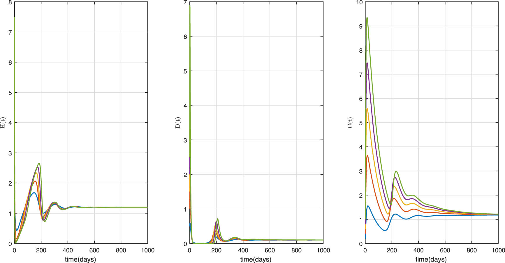
Time evolution of the local banking system under the influence of rumor with

Time evolution of the local banking system under the influence of rumor with
4.2 Optimal paths
We proved in Section 3, Theorem 3.1, the existence and uniqueness of optimal solution of problem (71) for small time. We also gave the characterizations of optimal controls in Theorem 3.2. In what follows, we use the shooting method implemented on MATLAB software to illustrate these results.
Figure 6 gives the profiles of the optimal control. Figure 7 displays the optimal states trajectories. We can observe that without control the healthy banks can be reduced significantly, which is prejudicious for the stability of the financial system and even for the development of the economy. The control allows to maintain a minimum level of healthy banks in the banking system. We also observe that the rate of assistance to distressed banks is greater than that of banks in crisis. An explanation is that, due to the fact that distressed banks contribute to spread the stress (it is not the case for banks in crisis), it is more efficient to assist them in order to contain the crisis.

Optimal controls paths

Optimal behavior of the banking system with
5 Conclusion
The bank run phenomenon, most often originated from the rumor about the financial health of given banks, can create important damage on a banking system. In the literature, many theoretical and empirical studies have been made on the spread of the financial crisis. However, to the best of our knowledge, no theoretical model of the impact of rumors on the propagation of the banking crisis has been made. In this paper, we proposed a mathematical model based on an epidemiological approach of the above problem. Our main findings are summarized below.
By using a Lyapunov function and a comparison Theorem, we studied the asymptotic behavior of the submodel of rumor spread.
A sensitivity study allowed us to highlight the importance of the parameters
We obtained conditions under which stressed banks disappear or persist in the banking system.
To contain the disastrous effects of rumor spread on the stability of the financial system, we proposed and solved an optimal control problem with the objective of minimizing, at the lowest cost, the number of distressed banks and banks in crisis. The results obtained can be useful to regulators in developing strategies to maintain financial stability.
All the aforementioned findings are illustrated by numerical simulations.
Acknowledgements
The authors would like to thank the three anonymous referees for their comments and suggestions, which helped greatly improve the manuscript.
-
Funding information: The authors state no funding involved.
-
Author contributions: All authors have accepted responsibility for the entire content of this manuscript and approved its submission.
-
Conflict of interest: The authors state no conflict of interest.
References
[1] F. Allen and D. Gale, Financial contagion, J. Polit. Econ. 108 (2000), no. 1, 1–33. 10.1086/262109Search in Google Scholar
[2] K. Anand, P. Gai, and M. Marsilli, Contagion in financial networks, J. Econom. Dynam. Control 36 (2012), no. 8, 1088–1100. 10.1016/j.jedc.2012.03.005Search in Google Scholar
[3] E. Nier, J. Yang, and T. Yorulmazer, Network models and financial stability, J. Econom. Dynam. Control 31 (2007), no. 6, 2033–2060. 10.1016/j.jedc.2007.01.014Search in Google Scholar
[4] B. Martin, T. Stefan, and V. Razvan, Understanding bank-run contagion, ECB Working Paper Number, 1711, 2014. Search in Google Scholar
[5] B. Fred, Mathematical epidemiology: Past, present, and future, Infect. Dis. Model. 2 (2017), 113–127. 10.1016/j.idm.2017.02.001Search in Google Scholar
[6] Z. Ma, X. Jiaotong, and J. Li, Dynamical Modeling and Analysis of Epidemics, World Scientific Publishing, Singapore, 2009. 10.1142/6799Search in Google Scholar
[7] J. R. Piquera and V. O. Araujo, A modified epidemiological model for computer viruses, Appl. Math. Comput. 213 (2009), 335–360. 10.1016/j.amc.2009.03.023Search in Google Scholar
[8] K. Afassinou, Analysis of the impact of education rate on the rumor spreading mechanism, Phys. A 414 (2014), 43–52. 10.1016/j.physa.2014.07.041Search in Google Scholar
[9] Y. Hu, Q. Pan, W. Hou, and M. He, Rumor spreading model considering the proportion of wisemen in crowd, Phys. A 505 (2018), 1084–1094. 10.1016/j.physa.2018.04.056Search in Google Scholar
[10] M. Li, H. Zhang, P. Georgescu, and T. Li, The stochastic evolution of a rumor spreading model with two distinct spread inhibiting and attitude adjusting mechanisms in a homogeneous social network, Phys. A 562 (2021), 1–24. 10.1016/j.physa.2020.125321Search in Google Scholar PubMed PubMed Central
[11] M. Toivanen, Contagion in the interbank network: an epidemiological approach, Bank of Finland Research Discussion Papers, 19, 2003. 10.2139/ssrn.2331300Search in Google Scholar
[12] O. Kostylenko, H. S. Rodrigues, and D. F. Torres, Banking risk as an epidemiological model: an optimal control approach, Springer Proc. Math. Stat. 223 (2017), 165–176. 10.1007/978-3-319-71583-4_12Search in Google Scholar
[13] A. Bucci, D. LaTorre, D. Liuzzi, and S. Marsiglio, Financial contagion and economic development: an epidemiological approach, J. Econ. Behav. Organ. 162 (2019), no. 1, 211–228. 10.1016/j.jebo.2018.12.018Search in Google Scholar
[14] U. S. code Title 11-Bankruptcy, https://www.law.cornell.edu [Accessed 6 March 2021]. Search in Google Scholar
[15] COBAC, Regulation No 02/14 /CEMAC/ UMAC/COBAC of 25 April 2014, COBAC, 2014. Search in Google Scholar
[16] W. Wagner, In the quest of systemic externalities: a review of the literature, CESifo Econ. Stud. 56 (2010), no. 1, 96–111. 10.1093/cesifo/ifp022Search in Google Scholar
[17] J. Müller, Interbank credit lines as a channel of contagion, J. Financial Serv. Res. 29 (2006), no. 1, 37–60. 10.1007/s10693-005-5107-2Search in Google Scholar
[18] D. W. Diamond and P. H. Dybvig, Bank runs, deposit insurance, and liquidity, J. Polit. Econ. 91 (1983), no. 3, 401–419. 10.1086/261155Search in Google Scholar
[19] R. J. Caballero and A. Krishnamurthy, Collective risk management in a flight to quality episode, J. Finance 63 (2008), no. 5, 2195–2230. 10.3386/w12896Search in Google Scholar
[20] S. Brusco and F. Castiglionesi, Liquidity coinsurance, moral hazard, and financial contagion, J. Finance 62 (2000), no. 5, 2275–2302. 10.1111/j.1540-6261.2007.01275.xSearch in Google Scholar
[21] P. Gai and A. H. S. Kapadia, Complexity, concentration and contagion, J. Monet. Econ. 58 (2011), no. 5, 453–470. 10.1016/j.jmoneco.2011.05.005Search in Google Scholar
[22] P. Glasserman and H. P. Young, Contagion in financial networks, J. Econ. Lit. 54 (2016), no. 3, 779–831. 10.1257/jel.20151228Search in Google Scholar
[23] X. Liao, L. Wang, and P. Yu, Stability of dynamical systems, Monograph Series on Nonlinear Science and Complexity, vol. 5, 2007. 10.1016/S1574-6917(07)05001-5Search in Google Scholar
[24] J. K. Hale and S. M. VerduynLunel, Introduction to Functional Differential Equations, Springer-Verlag, New York, 1993. 10.1007/978-1-4612-4342-7Search in Google Scholar
[25] V. Lakshmikantham, S. Leela, and A. A. Matynyuk, Stability Analysis of Nonlinear Systems, Marcel Dekker Inc., New York and Basel, 1989. Search in Google Scholar
[26] D. Philippas, Y. Koutelidakis, and A. Leontitsis, Insights into european interbank network contagion, Manag. Finance 41 (2015), no. 8, 754–772. 10.1108/MF-03-2014-0095Search in Google Scholar
[27] W. H. Fleming and R. W. Rishel, Deterministic and Stochastic Optimal Control, Springer, Berlin, 1975. 10.1007/978-1-4612-6380-7Search in Google Scholar
[28] H. Gaff and E. Schaefer, Optimal control applied to vaccination and treatment strategies for various epidemiological models, Math. Biosci. Eng. 6 (2009), no. 3, 469–492. 10.3934/mbe.2009.6.469Search in Google Scholar PubMed
[29] S. P. Sethi, Optimal Control Theory: Applications to Management Science and Economics, Springer Nature Switzerland AG, 2019. 10.1007/978-3-319-98237-3Search in Google Scholar
[30] J. Zabczyk, Mathematical Control Theory: An Introduction, Birkhäuser, Boston, 1995. Search in Google Scholar
[31] E. R. Avakov, The maximum principle for abnormal optimal control problems, Akademiia Nauk SSSR Doklady 298 (1988), no. 6, 1289–1292. Search in Google Scholar
© 2022 Calvin Tadmon and Eric Rostand Njike-Tchaptchet, published by De Gruyter
This work is licensed under the Creative Commons Attribution 4.0 International License.
Articles in the same Issue
- Regular Articles
- On some summation formulas
- A study of a meromorphic perturbation of the sine family
- Asymptotic behavior of even-order noncanonical neutral differential equations
- Unconditionally positive NSFD and classical finite difference schemes for biofilm formation on medical implant using Allen-Cahn equation
- Starlike and convexity properties of q-Bessel-Struve functions
- Mathematical modeling and optimal control of the impact of rumors on the banking crisis
- On linear chaos in function spaces
- Convergence of generalized sampling series in weighted spaces
- Persistence landscapes of affine fractals
- Inertial iterative method with self-adaptive step size for finite family of split monotone variational inclusion and fixed point problems in Banach spaces
- Various notions of module amenability on weighted semigroup algebras
- Regularity and normality in hereditary bi m-spaces
- On a first-order differential system with initial and nonlocal boundary conditions
- On solving pseudomonotone equilibrium problems via two new extragradient-type methods under convex constraints
- Local linear approach: Conditional density estimate for functional and censored data
- Some properties of graded generalized 2-absorbing submodules
- Eigenvalue inclusion sets for linear response eigenvalue problems
- Some integral inequalities for generalized left and right log convex interval-valued functions based upon the pseudo-order relation
- More properties of generalized open sets in generalized topological spaces
- An extragradient inertial algorithm for solving split fixed-point problems of demicontractive mappings, with equilibrium and variational inequality problems
- An accurate and efficient local one-dimensional method for the 3D acoustic wave equation
- On a weighted elliptic equation of N-Kirchhoff type with double exponential growth
- On split feasibility problem for finite families of equilibrium and fixed point problems in Banach spaces
- Entire and meromorphic solutions for systems of the differential difference equations
- Multiplication operators on the Banach algebra of bounded Φ-variation functions on compact subsets of ℂ
- Mannheim curves and their partner curves in Minkowski 3-space E13
- Characterizations of the group invertibility of a matrix revisited
- Iterates of q-Bernstein operators on triangular domain with all curved sides
- Data analysis-based time series forecast for managing household electricity consumption
- A robust study of the transmission dynamics of zoonotic infection through non-integer derivative
- A Dai-Liao-type projection method for monotone nonlinear equations and signal processing
- Review Article
- Remarks on some variants of minimal point theorem and Ekeland variational principle with applications
- Special Issue on Recent Methods in Approximation Theory - Part I
- Coupled fixed point theorems under new coupled implicit relation in Hilbert spaces
- Approximation of integrable functions by general linear matrix operators of their Fourier series
- Sharp sufficient condition for the convergence of greedy expansions with errors in coefficient computation
- Approximation of conic sections by weighted Lupaş post-quantum Bézier curves
- On the generalized growth and approximation of entire solutions of certain elliptic partial differential equation
- Existence results for ABC-fractional BVP via new fixed point results of F-Lipschitzian mappings
- Linear barycentric rational collocation method for solving biharmonic equation
- A note on the convergence of Phillips operators by the sequence of functions via q-calculus
- Taylor’s series expansions for real powers of two functions containing squares of inverse cosine function, closed-form formula for specific partial Bell polynomials, and series representations for real powers of Pi
- Special Issue on Recent Advances in Fractional Calculus and Nonlinear Fractional Evaluation Equations - Part I
- Positive solutions for fractional differential equation at resonance under integral boundary conditions
- Source term model for elasticity system with nonlinear dissipative term in a thin domain
- A numerical study of anomalous electro-diffusion cells in cable sense with a non-singular kernel
- On Opial-type inequality for a generalized fractional integral operator
- Special Issue on Advances in Integral Transforms and Analysis of Differential Equations with Applications
- Mathematical analysis of a MERS-Cov coronavirus model
- Rapid exponential stabilization of nonlinear continuous systems via event-triggered impulsive control
- Novel soliton solutions for the fractional three-wave resonant interaction equations
- The multistep Laplace optimized decomposition method for solving fractional-order coronavirus disease model (COVID-19) via the Caputo fractional approach
- Special Issue on Problems, Methods and Applications of Nonlinear Analysis
- Some recent results on singular p-Laplacian equations
- Infinitely many solutions for quasilinear Schrödinger equations with sign-changing nonlinearity without the aid of 4-superlinear at infinity
- Special Issue on Recent Advances for Computational and Mathematical Methods in Scientific Problems
- Existence of solutions for a nonlinear problem at resonance
- Asymptotic stability of solutions for a diffusive epidemic model
- Special Issue on Computational and Numerical Methods for Special Functions - Part I
- Fully degenerate Bernoulli numbers and polynomials
- Wigner-Ville distribution and ambiguity function associated with the quaternion offset linear canonical transform
- Some identities related to degenerate Stirling numbers of the second kind
- Two identities and closed-form formulas for the Bernoulli numbers in terms of central factorial numbers of the second kind
- λ-q-Sheffer sequence and its applications
- Special Issue on Fixed Point Theory and Applications to Various Differential/Integral Equations - Part I
- General decay for a nonlinear pseudo-parabolic equation with viscoelastic term
- Generalized common fixed point theorem for generalized hybrid mappings in Hilbert spaces
- Computation of solution of integral equations via fixed point results
- Characterizations of quasi-metric and G-metric completeness involving w-distances and fixed points
- Notes on continuity result for conformable diffusion equation on the sphere: The linear case