Home Persistence landscapes of affine fractals
Article Open Access

Persistence landscapes of affine fractals

  • Michael J. Catanzaro , Lee Przybylski and Eric S. Weber EMAIL logo
Published/Copyright: May 27, 2022
Become an author with De Gruyter Brill

Abstract

We develop a method for calculating the persistence landscapes of affine fractals using the parameters of the corresponding transformations. Given an iterated function system of affine transformations that satisfies a certain compatibility condition, we prove that there exists an affine transformation acting on the space of persistence landscapes, which intertwines the action of the iterated function system. This latter affine transformation is a strict contraction and its unique fixed point is the persistence landscape of the affine fractal. We present several examples of the theory as well as confirm the main results through simulations.

MSC 2010: 55N31; 28A80; 37M22; 47H09

1 Introduction

Affine fractals are the invariant set of an iterated function system (IFS) consisting of affine transformations acting on Euclidean space. Well-known examples of such fractals are Cantor sets and Mandelbrojt sets. Affine fractals, as subsets of Euclidean space, possess topological properties that can be extracted through the methods of algebraic topology. In particular, these subsets of Euclidean space can be associated with a persistence landscape [1], which is a sequence of functions that encode geometric properties of the set based on Euclidean distances. These distances give rise to a family of homology groups derived from a filtration of complexes. The homology groups in turn produce a persistence module from which the persistence landscapes are defined.

Interest in studying fractals using the tools of algebraic topology has occurred recently. In [2], it was shown that persistence homology can be used to distinguish fractals of the same Hausdorff dimension. In [3], the authors describe a relationship between the Hausdorff dimension of fractals and the persistence intervals of Betti numbers.

Our main result (Theorem 4) concerns the calculation of the persistence diagrams and landscapes of affine fractals. We prove that, under a certain compatibility condition, there exists an affine transformation , which is defined by the parameters of the IFS. This transformation acts on the space of persistence landscapes. Moreover, it is a strict contraction and its unique fixed point is the persistence landscape of the affine fractal. Consequently, the persistence landscape of the fractal can be computed via the limiting process of repeated applications of to any initial input. We also prove, under an additional assumption on the IFS, that intertwines the action of the iterated function system (Theorem 5).

1.1 Persistence landscapes

Persistent homology is a relatively new approach to studying topological spaces. In the context of data science, persistent homology can be applied to a data set to complement traditional statistical approaches by studying the geometry of the data. We employ the tools of persistent homology, including persistence landscapes, to analyze affine fractals.

Persistent homology typically begins with a set of points, equipped with a pairwise notion of distance. We place a metric ball of radius r around each point and increase r . We are interested in the topological properties of the union of these balls as a function of r. Typical properties of interest include connectedness, loops or holes, and voids of the union, and importantly the radii at which these appear or disappear. While this type of information may seem crude, a surprising amount of insight about the underlying set of points can be extracted in this way.

The data of changing topological properties are conveniently summarized in what is known as a persistence diagram, a multiset of points in the plane. If we focus on loops of the union, then each point ( b , d ) in the persistence diagram represents a loop, whose two coordinates correspond to the radius when the hole is formed ( r = b ) and when it gets filled in ( r = d ). The persistence diagram provides a multiscale summary, encoding geometric and topological features of the set [4].

Unfortunately, however, barcodes do not possess a vector space structure, and so the quantitative analysis and precise comparison can be difficult [5]. To remedy this, we map the barcodes to some feature space (a Banach space in our case) using a well-studied feature map known as a persistence landscape. The mapping from barcodes to landscapes is reversible, and so this vectorization scheme loses no information [1]. Persistence landscapes have been used to study protein binding [6], phase transitions [7], audio signals [8], and microstructures in materials science [9].

See Section 2 for a full discussion of persistent homology and persistence landscapes of metric spaces.

1.2 Affine fractals

A fractal, for our purposes, is a set that has a self-similarity property. The middle-third Cantor set is the canonical example of a self-similar set. Fractals are commonly studied objects in many contexts. Cantor sets, in particular, appear in the context of analysis [10,11], number theory [12,13], probability [14,15,16], geometry [17,18], physics [19,20,21], and harmonic analysis [22,23,24].

In this paper, we consider specifically the class of affine fractals, which are generated by iterated function systems consisting of affine transformations. By this, we mean that the fractal is the invariant set for the iterated function system.

Definition 1

Suppose Ψ = { ψ 1 , , ψ N } is a set of maps acting on a metric space ( X , d ) . We say that A X is invariant for Ψ if A = i = 1 N ψ i ( A ) .

For the maps Ψ , we denote the compositions (i.e. iterations) of the maps by:

Ψ ( A ) = i = 1 N ψ i ( A ) , Ψ p ( A ) = Ψ ( Ψ p 1 ( A ) ) .

In [25], Hutchinson laid out the main relationship between fractals and iterated function systems (IFS); this relationship is the foundation of our results. Recall that ψ : X X is Lipschitz if for all x , y X , there exists C > 0 such that

d ( ψ ( x ) , ψ ( y ) ) C d ( x , y ) .

The Lipschitz constant of ψ is the infimum of all such C . We say that ψ is a contraction if it has Lipschitz constant less than 1. Hutchinson’s theorem is as follows.

Theorem A

Let X = ( X , d ) be a complete metric space and Ψ = { ψ 1 , , ψ N } a finite set of contraction maps on X. Then there exists a unique closed bounded set A such that

A = i = 1 N ψ i ( A ) .

Furthermore, A is compact and is the closure of the set of fixed points of finite compositions of members of Ψ . Moreover, for a closed bounded K , Ψ p ( K ) A in the Hausdorff metric.

Recall that the Hausdorff distance between two sets A , B X is given by

d H ( A , B ) = max { sup x A inf y B d ( x , y ) , sup y B inf x A d ( x , y ) } .

For us, the maps Ψ consist of affine transformations acting on R d . Moreover, we assume that the linear part of the maps are scalars that are common to all of the maps. Therefore, our maps have the form ψ j ( x ) = c ( x + b j ) , where c ( 0 , 1 ) . The followings are examples of affine fractals in our class:

  1. The classical middle-third Cantor set in R ;

  2. The Sierpinski gasket in R 2 ;

  3. The Sierpinski carpet in R 2 ;

  4. The Menger sponge (or Sierpinski cube) in R 3 .

Specifically, the Cantor set is the invariant set for the IFS with generators

ψ 0 ( x ) = x 3 ; ψ 1 ( x ) = x + 2 3 .

Likewise, the Sierpinski carpet is the invariant set for the IFS with generators

ψ 0 ( x , y ) = x 3 , y 3 ; ψ 1 ( x ) = x + 2 3 , y 3 ; ψ 2 ( x ) = x 3 , y + 2 3 ; ψ 3 ( x ) = x + 2 3 , y + 2 3 .

For an IFS Ψ acting on R d and a nonempty S 0 R d , we define the sequence S n + 1 = Ψ ( S n ) . We will typically consider S 0 , which consists of finitely many points in R d , and therefore by Hutchinson’s theorem, { S n } converges in the Hausdorff metric to the fractal generated by Ψ . Indeed, we will show that choosing S 0 to be the extreme points of the convex hull of the fractal is ideal in establishing our algorithm for calculating the persistence landscapes of the fractal.

One of our main results is to prove that for a fixed affine IFS Ψ that satisfies a certain compatibility condition and appropriate initialization S 0 , there exists an affine transformation acting on the space of persistence landscapes such that for every n N , the following diagram commutes:

(1)

Here, f n is the persistence landscape of S n and γ associates with S n its persistence landscape. We will show that is a strict contraction on the set of persistence landscapes, and so it possesses a unique fixed point. That fixed point will be the persistence landscape for the fractal generated by Ψ . Consequently, the persistence landscape f of the fractal is obtained by

(2) f = lim n n f 0

for any initialization f 0 .

2 Persistent homology

In this section, we briefly review some standard facts from algebraic topology and persistent homology as well as establish our notation. Excellent resources for (simplicial) homology can be found in [26,27], and [4,28,29] provide a good introduction to persistent homology.

2.1 Simplicial complexes

For a simplicial complex K , the p-skeleton of K, denoted by K ( p ) , is the subcomplex consisting of all simplices of dimension less than or equal to p . The set of all p -simplices is denoted K p . Thus, the set of vertices can be written as K 0 . Recall that if σ = [ u 0 , u 1 , , u p ] is a p -simplex, then every point x σ can be expressed as a convex combination x = i α i u i , where 0 α i 1 and i α i = 1 .

Given two simplicial complexes K and L , we say that φ : K 0 L 0 is a vertex map if for any p -simplex [ x 0 , , x p ] in K , [ φ ( x 0 ) , , φ ( x p ) ] is a simplex in L . Thus, vertex maps send the vertices of simplices in K to simplices in L . We do not require φ to be injective, so dim [ φ ( x 0 ) , , φ ( x p ) ] p with a strict inequality if φ ( x j ) = φ ( x k ) for some j , k { 0 , 1 , , p } . Given a vertex map φ : K 0 L 0 , we can extend it to a map f : K L by

f ( x ) = j = 0 p α j φ ( x j ) ,

where x = j = 0 p α j x j . In this way, we say that f is the simplicial map induced by φ .

The first step in our goal of computing topological properties of affine fractals will be to construct their Cěch complexes. If X R d , for any ε > 0 , we can define the Cěch complex to be

(3) Cěch ( X , ε ) = { σ X x σ B ( x , ε / 2 ) ¯ } ,

where B ( x , r ) is the ball of radius r centered at x . A consequence of the Nerve theorem [28,30] is that for a finite set X R d , { x : d ( x , X ) ε / 2 } is homotopy equivalent to Cěch ( X , ε ) .

There is another popular variant in persistent homology for associating a topological space with a set, known as the Vietoris-Rips complex. The Vietoris-Rips complex for X R d and ε > 0 is defined by

(4) VR ( X , ε ) = { σ X max x , y σ x y ε } .

In comparing equations (3) and (4), we see that the 1-simplices in Cěch ( X , ε ) are the same as those in VR ( X , ε ) , but it is not necessary that Cěch ( X , ε ) = VR ( X , ε ) . Furthermore, verifying the existence of a point in the intersection of equation (3) often requires much more work than verifying the pairwise condition of equation (4). For this reason, together with recent advances in computational efficiency in software [31], applications of persistent homology tend to rely on Vietoris-Rips complexes. The two complexes are related by a well-known result [32, Thm. 2.5].

Our focus will be on the Cěch complex of affine fractals and their approximations.

2.2 A review of homology

Given a simplicial complex K , an Abelian group G , and a nonnegative integer p 0 , we define the group of p-chains with coefficients in G to be formal G -linear combinations of p -simplices of K and denote it C p ( K ; G ) . A typical element of C p ( K ; G ) is a finite formal sum of the form i g i σ i , where σ i K p and g i G . The differential (or boundary) of a p -simplex σ = [ u 0 , u 1 , , u p ] is expressed as follows:

(5) p ( σ ) = j = 0 p ( 1 ) j [ u 0 , u 1 , , u ˆ j , , u p ] C p 1 ( K ; G ) ,

where [ u 0 , , u ˆ j , , u p ] is the ( p 1 ) -simplex obtained by omitting u ˆ j from σ . Extending p to a G -linear homomorphism to all of C p ( K ; G ) gives p : C p ( K ; G ) C p 1 ( K ; G ) . This gives rise to the simplicial chain complex of K with coefficients in G

(6) p + 2 C p + 1 ( K ) p + 1 C p ( K ) p C p 1 ( K ) p 1 1 C 0 ( K ) 0 0 ,

with the essential property that any two successive compositions equal the trivial map: j j + 1 = 0 for all j 0 . Hence, im ( j + 1 ) ker ( j ) . We denote the p-cycles by Z p ( K ) = ker ( p ) C p ( K ) , and the p-boundaries by B p ( K ) = im ( p + 1 ) C p ( K ) .

Definition 2

The p th simplicial homology group of a simplicial complex K is expressed as follows:

H p ( K ) = H p ( K ; G ) ker ( p ) / im ( p + 1 ) = Z p ( K ) / B p ( K ) .

We let H ( K ) = p H p ( K ) denote the collection of homology groups for all dimensions p .

Moving forward, we assume G = Z 2 . This choice of coefficients is common in persistent homology and simplifies many of the computations, e.g., the factors of ( 1 ) j appearing in equation (5) vanish.

For simplicial complexes K and L , f : K L is a simplicial map if f is continuous and f maps each simplex of K linearly onto a simplex of L . Define a homomorphism f # : C p ( K ) C p ( L ) by first defining

(7) f # ( [ x 0 , , x p ] ) = [ f ( x 0 ) , , f ( x p ) ] if f ( x 0 ) , , f ( x p ) are distinct , 0 otherwise

and extend the homomorphism to the rest of C p ( K ) linearly. A standard fact in algebraic topology is that f # further induces a map on homology f : H p ( K ) H p ( L ) for every p . Furthermore, if f is a simplicial homeomorphism, then f : H ( K ) H ( L ) is an isomorphism [27].

Lemma 1

Let X R d be a finite point cloud. Let φ : R d R d be a similitude with scaling constant c > 0 . Let ε > 0 , L = Cěch ( X , ε ) , and let L ˜ = Cěch ( φ ( X ) , c ε ) . Then φ L 0 : L 0 L ˜ 0 is a vertex map and induces a simplicial homeomorphism f between L and L ˜ . Thus, f induces an isomorphism f : H ( L ) H ( L ˜ ) .

A particularly nice feature of homology groups is that the homology group of a space is isomorphic to the direct sum of the homology groups of the path components [26, Prop. 2.6]. This directly leads to the following lemma.

Lemma 2

Let X R d be a finite subset and { φ j } j = 1 n be a collection of similitudes on R d . Let c j equal the scaling constant of the similitude φ j . Define

δ min 1 j k n d ( φ ( X j ) , φ ( X k ) ) .

Then for all dimensions p 0 , and all ε < δ

H p Cěch ( j φ j ( X ) , ε ) j = 1 n H p Cěch ( X , c j 1 ε ) .

Lemma 2 implies that given a finite point cloud and a collection of similitudes, so long as the images of the point cloud under those similitudes are sufficiently far apart, the homology group resulting from the union of those images is easily related to the homology groups resulting from the original point cloud.

Another tool we will use for the computation of homology groups is known as the Mayer-Vietoris sequence. Suppose K is a simplicial complex with subcomplexes K 1 and K 2 such that K = K 1 K 2 . The Mayer-Vietoris sequence is the long exact sequence:

(8) H p ( K 1 K 2 ) H p ( K 1 ) H p ( K 2 ) H p ( K ) H p 1 ( K 1 K 2 ) H 0 ( K 1 K 2 ) H 0 ( K 1 ) H 0 ( K 2 ) H 0 ( K ) 0 .

For a detailed explanation of the maps in the sequence and a proof of its exactness, see [27, Chapter 3].

2.3 Persistent homology

A simplicial filtration K of a simplicial complex K is a collection of subcomplexes { K i } i I , for an indexing set I R such that whenever s t ,

(9) K s K t K .

The inclusion map K s K t induces a homomorphism H ( K s ) H ( K t ) . The collection of groups { H p ( K s ) } s I , together with the collection of homomorphisms { H p ( K s ) H p ( K t ) } s t form the p th -persistent homology of K .

Understanding the structure of persistent homology is difficult as presented. Instead, we turn to a generalization of this structure known as a persistence module. A persistence module is a collection of Z 2 -vector spaces V = { V t } t I , and a collection of linear transformations between these spaces M = { M s , t : V s V t } s t that satisfy

(10) M s , t M r , s = M r , t for r s t .

We will often refer to the persistence module ( V , M ) as simply M . By setting V s = H p ( K s ) and M s , t : H p ( K s ) H p ( K t ) as the homomorphism induced by inclusion, we see that every simplicial filtration K gives rise to a persistence module.

If X R d , then the collection of simplicial complexes

Cěch ( X ) = { Cěch ( X , s ) } s R ¯

form a simplicial filtration of Cěch ( X , ) , the full simplicial complex on X . For 0 s t , the inclusion mapping Cěch ( X , s ) Cěch ( X , t ) induces a homomorphism H p Cěch ( X , s ) H p Cěch ( X , t ) . We let H p Cěch ( X ) denote the persistence module resulting from the filtration of the Cěch complex of X . We adopt the convention that

Cěch ( X , s ) = VR ( X , s ) =

for s < 0 .

A persistence diagram is a multiset of birth and death times derived from a decomposition of a persistence module. Interval modules form the basic building blocks of persistence modules. Interval modules are indecomposable. In [33], it was shown that the persistence module ( V , M ) can be decomposed into interval modules as long as each V t is finite dimensional. Moreover, an application of [34, Thm. 1], implies that this decomposition is unique, up to reordering. Thus, if we have a persistence module M with the interval module decomposition

M = λ J [ b λ , d λ ) ,

and we define the persistence diagram of M to be the multiset

dgm M = { ( b λ , d λ ) } λ Δ ,

where Δ is the set of diagonal points { ( x , x ) x R } each counted with infinite multiplicity.

We will denote a persistence diagram as D = ( D , μ ) , where D = { ( b λ , d λ ) } λ is the collection of distinct birth and death times and μ : D N 0 is defined μ ( b λ , d λ ) as the multiplicity of the birth death time ( b λ , d λ ) .

To ensure that the persistence modules we consider have a decomposition into interval modules, we require that M is q-tame [35].

Definition 3

The persistence module ( V , M ) indexed over I R is said to be q-tame if

rank M s , t < whenever s < t .

Assuming a persistence module is q-tame guarantees us not only a well-defined persistence diagram, but also stability with respect to the bottleneck distance [36]. A prior stability result was presented by Cohen-Steiner et al. in [37], which required a more restrictive tameness condition.

Persistence modules resulting from a Cěch filtration built on a finite point cloud X are q -tame. Moreover, when X R d is compact, H p Cěch ( X ) is q -tame [38] for all p . As a result, we obtain the following:

Proposition 1

For any affine iterated function system, the invariant set A and any finite approximation of A , possess a well-defined persistence diagram.

While persistence diagrams are an effective representation of a persistence module, they are not conducive to statistical analysis. Persistence landscapes address this issue by embedding persistence diagrams into a Banach space. Given a persistence module M that is q -tame, its persistence landscape is a function f : N × R R ¯ by

f ( n , t ) f ( n ) ( t ) = sup { m 0 rank M t m , t + m n } ,

where R ¯ denotes the extended real numbers, [ , ] . We have that all persistence landscapes are elements of

L ( N × R ) { g = { g ( n ) } n = 1 L ( R ) sup n N g ( n ) L ( R ) < } .

We compute the distance between two persistence landscapes using the standard norm on L ( N × R ) , which is defined as follows:

g L ( N × R ) = sup n N g ( n ) L ( R ) .

There is an alternative definition given in [39] that allows us to relate the persistence landscape of M to its persistence diagram. If the persistence module M is represented as a persistence diagram D = { ( a i , b i ) } i I , then we can define the functions

(11) τ ( a , b ) ( t ) = max ( 0 , min ( a + t , b t ) ) ,

and for all k N , t R ,

(12) f ( k ) ( t ) = kmax { τ ( a i , b i ) ( t ) } i I .

We use kmax to denote the k th largest element of a set. Note that since D is a multiset, certain birth death pairs ( a i , b i ) can appear more than once.

It is common for many stability results to write the distance between two persistence landscapes in terms of their corresponding persistence modules. If f = { f ( k ) } k = 1 is the persistence landscape obtained from M and g = { g ( k ) } k = 1 is the persistence landscape obtained from M , we define the persistence landscape distance between M and M to be

(13) Λ ( M , M ) f g L ( N × R ) .

By combining the stability results from [1,38,36], we obtain the following:

Theorem B

Suppose X is a metric space, and Y , Z X have well-defined persistence diagrams. Then for all p 0 ,

Λ ( H p Cěch ( Y ) , H p Cěch ( Z ) ) d H ( Y , Z ) .

Corollary 1

Let ( X , d ) be a metric space and suppose S , T X such that their Cěch complexes have well-defined persistence diagrams. Then

f g L ( N × R ) d H ( S , T ) ,

where f and g are the persistence landscapes of S and T, respectively.

3 The persistence landscapes of affine fractals

3.1 The persistence landscape of the Cantor set

We begin with calculating the persistence landscape of the middle-third Cantor set C . This calculation illustrates the main ideas of our construction, while also highlighting some of the technical requirements on the IFS. Recall that C is generated by the IFS given by the collection of contraction maps Ψ = { ψ 0 , ψ 2 } , where

ψ 0 ( x ) = x 3 , ψ 2 ( x ) = x 3 + 2 3 .

For convenience, we suppose that Ψ acts on the metric space X = [ 0 , 1 ] with the standard metric. We define the sequence of approximations to C as follows:

(14) S 0 = { 0 , 1 } , S n = Ψ ( S n 1 ) = ψ 0 ( S n 1 ) ψ 2 ( S n 1 ) for n N .

We also define

C 0 = [ 0 , 1 ] , C n = Ψ ( C n 1 ) .

The length of each closed interval in C n is 1 / 3 n . Note that since the points in S n are equal to the end points in the disjoint closed intervals that make up C n , and we have S n C C n for all n N , we find

d H ( S n , C ) d H ( S n , C n ) 1 2 3 n .

As a consequence of this and Lemma 2.3, we obtain the following convergence result.

Theorem 1

Let { f n } n = 1 be the sequence of persistence landscapes generated from the sequence of point clouds { S n } n = 1 as in equation (14), and let f be the persistence landscape of C . Then, we have that

lim n f n f L ( N × R ) = 0 .

Knowing that the limit exists, we would still like to have a formula for the persistence landscape of C . To help us determine this formula, we will use a two-step approach. First, we will find an affine operator : L ( N × R ) L ( N × R ) such that for all n sufficiently large, maps the persistence landscape of S n to the persistence landscape of S n + 1 . We will then show that the persistence landscape of C is the fixed point of and use to compute the fixed point.

To describe persistence landscapes, we will use the hat functions defined in equation (11). Recall that persistence landscapes h L ( N × R ) are defined by letting h = { h ( j ) } j = 1 , where h ( j ) equals the j th largest hat function supported on an interval whose end points equal one of the birth-death pairs from the persistence diagram. We also note that the hat functions scale nicely so that for t R

τ ( a , b ) ( t ) = ( b a ) τ ( 0 , 1 ) ( ( b a ) 1 ( t a ) ) .

We define for each g L ( N × R ) by g = h = { h ( j ) } j = 1 , where

(15) h ( 1 ) ( x ) = τ ( 0 , 1 ) ( x ) , h ( 2 ) ( x ) = 1 3 g ( 1 ) ( 3 x ) , h ( 2 k + 1 ) ( x ) = h ( 2 k + 2 ) ( x ) = 1 3 g ( k ) ( 3 x ) , k N .

We adopt the convention that the maximum death time will be equal to the diameter of the invariant set, which in the case of C is 1. Thus, when computing persistence landscape of C , the first function in the sequence will be τ ( 0 , 1 ) . We can see that is an affine contraction. Indeed, if we define T : L ( N × R ) L ( N × R ) by T g = h , where

h ( 1 ) ( x ) = 0 , h ( 2 ) ( x ) = 1 3 g ( 1 ) ( 3 x ) h ( 2 k + 1 ) ( x ) = h ( 2 k + 2 ) ( x ) = 1 3 g ( k ) ( 3 x ) ,

and then we see that T is linear with T = 1 3 . Further, for all f L ( N × R ) , f = v + T f , where v = { τ ( 0 , 1 ) , 0 , 0 , 0 , } .

Theorem 2

Let { f n } n = 1 be the sequence of persistence landscape generated from the sequence of point clouds { S n } n = 1 as in equation (14), and let f be the persistence landscape of C . Let be given by equation (15). Then, for all n N , f n = f n + 1 .

In other words, the commutative diagram in equation (1) holds.

Proof

For n N , we denote f n = { f n ( j ) } j = 1 . It easy to check for n = 1 using direct computation. Since S 1 = { 0 , 1 } and S 2 = { 0 , 1 / 3 , 2 / 3 , 1 } we see that f 2 ( 1 ) = τ ( 0 , 1 ) , f 2 ( j ) = τ ( 0 , 3 1 ) for 2 j 4 , and f 2 ( j ) = 0 for all j > 4 . We can also see that

f 1 = { τ ( 0 , 1 ) , 0 , 0 , 0 , 0 , } .

By the definition of , we see that f 1 = f 2 . In general, for n N , let

L n = ϕ 0 ( S n ) , R n = ϕ 2 ( S n ) ,

as depicted in Figure 1. For all n N , we see that

S n + 1 = L n R n .

Since S n [ 0 , 1 ] , we know that L n R n = . Moreover,

(16) d ( L n , R n ) = min x L n , y R n x y = 1 3 .

Let D n = ( D n , μ n ) denote the persistence diagram of H 0 Cěch ( S n ) . Note that since S n has 2 n distinct points, if D n = { ( 0 , d j ) } j = 1 k , then j = 1 k μ n ( 0 , d j ) = 2 n . We assume without the loss of generality that d j < d j + 1 for j { 1 , , k } . This means d k = 1 , and for j < k , d j < 1 .

We claim that for j < k , ( 0 , d j ) D n implies that 0 , d j 3 D n + 1 with μ n + 1 ( 0 , d j / 3 ) = 2 μ n ( 0 , d j ) . To help us do this, we first prove that for 0 < ε < 1 , the diagram

(17)

commutes, where M 0 , ε and P 0 , ε are homomorphisms induced by the inclusions Cěch ( S n , 0 ) Cěch ( S n , ε ) and Cěch ( L n , 0 ) Cěch L n , ε 3 , respectively, and ϕ 0 0 and ϕ 0 ε are isomporphisms induced by ϕ 0 as in Corollary 1. Indeed, for γ H 0 Cěch ( S n , 0 ) , we may use coset notation to write γ = [ x ] B 0 ( Cěch ( S n , 0 ) ) for some x S n . Thus,

P 0 , ε ϕ 0 0 γ = P 0 , ε x 3 B 0 Cěch ( L n , 0 ) = x 3 B 0 Cěch L n , ε 3 .

On the other hand,

ϕ 0 ε M 0 , ε γ = ϕ 0 [ x ] B 0 Cěch ( S n , ε ) = x 3 B 0 Cěch L n , ε 3 .

Therefore, ϕ 0 ε M 0 , ε = P 0 , ε ϕ 0 0 , which implies diagram (17) commutes.

To prove the first claim, suppose ( 0 , d j ) D n with j < k , and then there are μ n ( 0 , d j ) distinct classes γ H 0 Cěch ( S n , 0 ) that die at d j . By assumption, there exists γ H 0 Cěch ( S n , 0 ) such that γ ker M 0 , d j , but γ ker M 0 , t , for t < d j . Let γ = ϕ 0 0 γ . Since the diagram in (17) commutes, γ ker P 0 , ε if and only if γ ker M 0 , ε . Thus, γ ker P 0 , d j , but γ ker P 0 , t for t < d j .

For s t , let Q s , t : H 0 Cěch R n , s 3 H 0 Cěch R n , t 3 be the homomorphism induced by the natural inclusion. By replacing L n with R n , and x 3 with x + 2 3 in the argument mentioned earlier, we can see that there also exists γ + H 0 Cěch ( R n , 0 ) such that γ + ker Q 0 , d j , but γ + ker Q 0 , t for t < d j . Since Cěch ( L n , ε ) is not path connected to Cěch ( R n , ε ) in Cěch ( S n + 1 , ε ) for ε < 1 3 , it follows that

H 0 Cěch ( S n + 1 , ε ) H 0 Cěch ( L n , ε ) H 0 Cěch ( R n , ε ) .

For 0 s t < 1 3 , the homomorphism F s , t : H 0 Cěch S n + 1 , s 3 H 0 Cěch S n + 1 , t 3 induced by the obvious inclusion satisfies

ker F s , t ker P s , t ker Q s , t .

Thus, for every class γ H 0 Cěch ( S n , 0 ) with death time d j < 1 , there exist two distinct classes in H 0 Cěch ( S n + 1 ) with death time d j 3 , which implies 0 , d j 3 D n + 1 with μ n + 1 0 , d j 3 = 2 μ n ( 0 , d j ) . This is equivalent to what we claimed.

It follows from our claim that

0 , d j 3 j = 1 k 1 D n + 1

and

j = 1 k 1 μ n + 1 0 , d j 3 = 2 j = 1 k 1 μ n ( 0 , d j ) = 2 ( 2 n 1 ) = 2 n + 1 2 .

By (16), we also see that ( 0 , 1 / 3 ) D n + 1 . Since we are working with the zero-dimensional homology of a Cěch complex, we also have ( 0 , 1 ) D n + 1 , since the space is nonempty. This accounts for all 2 n + 1 elements of D n + 1 . For convenience, we reindex D n and D n + 1 repeating elements according to their multiplicity and ordering them by decreasing death times so that

D n = { ( 0 , 1 ) , ( 0 , d ( 2 ) ) , ( 0 , d ( 3 ) ) , , ( 0 , d ( 2 n ) ) }

and

D n + 1 = { ( 0 , 1 ) , ( 0 , 1 / 3 ) , ( 0 , d ( 2 ) / 3 ) , ( 0 , d ( 2 ) / 3 ) , , ( 0 , d ( 2 n ) / 3 ) , ( 0 , d ( 2 n ) / 3 ) } .

Applying the definition in (12), we see that f n = { f n ( j ) } j = 1 , which is defined by

f n ( j ) = τ ( 0 , d ( j ) ) , for j { 1 , 2 , , 2 n } , and f n ( j ) = 0 for j > 2 n .

Since d ( 1 ) = 1 and d ( 2 ) = 1 / 3 , we easily check that f n + 1 = { f n + 1 ( j ) } j = 1 satisfies

f n + 1 ( 1 ) = τ ( 0 , 1 ) , f n + 1 ( 2 ) ( t ) = τ ( 0 , 1 / 3 ) ( t ) = 1 3 f n ( 1 ) ( 3 t ) f n + 1 ( 2 j + 1 ) ( t ) = f n + 1 ( 2 j + 2 ) ( t ) = τ ( 0 , d ( j ) / 3 ) ( t ) = 1 3 f j ( n ) ( 3 t ) for j N .

Therefore, f n = f n + 1 .□

Figure 1 


                                    S
                                 
                                 
                                    n


                           {S}_{n}
                        
                      divided into the components 


                                    L
                                 
                                 
                                    n


                           {L}_{n}
                        
                      and 


                                    R
                                 
                                 
                                    n


                           {R}_{n}
                        
                      for 


                              n
                              =
                              3
                           
                           n=3
                        
                     .
Figure 1

S n divided into the components L n and R n for n = 3 .

Since is Lipschitz with constant T = 1 3 < 1 , we see that has a unique fixed point and that unique fixed point is f = lim n f n , which is the persistence landscape function of C . The explicit formula for f can be found using by repeatedly applying to any vector in L ( N × R ) . We find that the persistence landscape of C is f = { f ( j ) } j = 0 , where

(18) f ( j ) = τ ( 0 , 1 ) if j = 1 , τ ( 0 , 3 k ) if 2 k 1 < j 2 k , k N .

We illustrate this landscape in Figure 2 (produced by pyscapes [40]).

Figure 2 
                  Graph of the functions 


                                    f
                                 
                                 
                                    2
                                 
                              
                              ,
                              
                                 …
                              
                              ,
                              
                                 
                                    f
                                 
                                 
                                    33


                           {f}_{2},\ldots ,{f}_{33}
                        
                      from the persistence landscape of the middle third Cantor set 


                              C
                           
                           {\mathcal{C}}
                        
                     .
Figure 2

Graph of the functions f 2 , , f 33 from the persistence landscape of the middle third Cantor set C .

We see from the illustration that the persistence landscape exhibits its own version of self-similarity. This is a reflection of the fact that the fractal contains several scaled copies of itself. Indeed, since scaling a subset of Euclidean space results in a proportional scaling of its persistence landscape, we should expect the persistence landscape of a fractal to contain a subsequence, which is a scaled copy of itself. The number of scaled copies, which corresponds to the number of generators of the IFS, is also reflected as a multiplicity in the persistence landscape.

3.2 Affine fractals with well-separated images and extreme points

The proof of Theorem 2 suggests that a more general result exists for an IFS satisfying certain properties. The two main ingredients that enable our calculations in the proof include (1) a judicious choice for the initial approximation S 0 and (2) a compatibility condition of the images of the maps in Ψ . We refer to this condition as well-separated images, and formalize this condition in Definition 4. We first consider the choice of S 0 . Before proceeding, we will need to introduce some notation and definitions. Unless stated otherwise, we assume Ψ = { ψ j } j = 1 N is an IFS consisting only of similitudes on R d with the form

(19) ψ j ( x ) = c ( x + b j ) , b j R d , c ( 0 , 1 ) .

We let A denote the invariant set of Ψ . For a set B R d , we let Conv( B ) denote the convex hull of B . We let E B denote the set of extreme points of Conv( B ). As we shall see, for the affine fractal A , choosing S 0 = E A is a good choice of initialization of our algorithm. This corresponds to the choice we made for the middle third Cantor set C ; see also the example in Section 4.4 for further evidence of this assertion.

Since the maps in Ψ are contractions, each map has a unique fixed element. Indeed, it is easy to calculate that for ψ j , the fixed point is x j = c 1 c b j . We let F A denote the set of these fixed points. Theorem A guarantees that F A A . The following result tells us that we can easily find E A .

Lemma 3

Suppose A R d is the invariant set for some IFS Ψ = { ψ j } j = 1 N consisting of similitudes of the form in equation (19). Then E A F A .

Proof

Let K = Conv ( A ) . Clearly, F A K . Assume F A = { x j } j = 1 N with x j = ψ j ( x j ) . We first observe that for j { 1 , , N } , since x j = c ( x j + b j ) , we know that c b j = ( 1 c ) x j . This implies that for j k ,

ψ k ( x j ) = c x j + c b k = c x j + ( 1 c ) x k Conv ( F A ) .

If y Conv ( F A ) , then for some t 1 , , t N 0 , j = 1 N t j = 1 we have

y = j = 1 N t j x j ,

and for any ψ k Ψ ,

ψ k ( y ) = c j = 1 N t j x j + b k = j = 1 N c t j x j + c b k = j = 1 N c t j x j + j = 1 N t j c b k = j = 1 N t j c ( x j + b k ) = j = 1 N t j ψ k ( x j ) .

Since ψ k ( x j ) Conv ( F A ) for all j { 1 , , N } , this implies that ψ k ( Conv ( F A ) ) Conv ( F A ) . Since k was arbitrary, this implies that the union of these images, Ψ ( Conv ( F A ) ) Conv ( F A ) . From Theorem A, we have

(20) A = lim p Ψ p ( Conv ( F A ) )

in the Hausdorff metric. We claim that A Conv ( F A ) . Indeed, choose x A . For all n N , it follows from equation (20) that there exists p ( n ) such that for some y n Ψ p ( n ) ( Conv ( F A ) ) ,

y n x 1 n .

Since Ψ p ( n ) ( Conv ( F A ) ) Conv ( F A ) for all n N , we have { y n } n = 1 Conv ( F A ) . Since Conv ( F A ) is a closed set and lim n y n = x , this implies x Conv ( F A ) , which proves the claim. Thus, we have the sequence of containment:

F A A Conv ( A ) Conv ( F A ) .

By definition, this implies Conv ( F A ) = Conv ( A ) . By the Krein-Milman theorem, it follows that

Conv ( F A ) = Conv ( A ) = Conv ( E A ) .

For any y E A , y Conv ( F A ) , it follows that y = j = 1 N t j x j , where j = 1 N t j = 1 . Since y is an extreme point, for some k { 1 , , N } , y = x k F A . Therefore, E A F A .□

One key property of C that was used in the proof of Theorem 2 was that at each scale, the set could be partitioned into a left and right set. The two halves were a significant distance away from each other, and each half was a scaled down version of the previous scale. This property can be described in terms of the IFS, and because of its usefulness, we will define it formally.

Definition 4

Let Ψ = { ψ j } j = 1 N be an IFS with invariant set A . We say that Ψ has well-separated images (or satisfies the well-separated condition) if

(21) min 1 j k N d ( ψ j ( A ) , ψ k ( A ) ) max 1 j N diam ψ j ( A ) .

This definition may apply to any IFS, not only those of the form given in equation (19). Note that on the left-hand side of the inequality, we have the usual Euclidean distance, not the Hausdorff distance.

3.3 Main results

By using the well-separated condition and the ideas in Section 3.1, we are now ready to elucidate the relationship between an IFS and the persistence landscape of its invariant set in more generality. Our main focus is on IFS with well-separated images having the form in equation (19), but many of the following results do not require these assumptions. We will use the same two-step approach that we used with C . We first identify a contraction on L ( N × R ) that has a fixed point equal to the persistence landscape of interest and then use the operator to find a formula for the persistence landscape. Theorem A implies that if Ψ is any IFS consisting of contractions then iteratively applying Ψ to any compact set K R d creates a sequence of compact sets, { S n } n = 1 , that converges to the invariant set A in the Hausdorff metric. Therefore, as a consequence of Theorem B:

Theorem 3

Let Ψ be an IFS on R d consisting of contractions with invariant set A . Let K R d be a compact set and define the sequence of compact sets { S n } n = 1 by

S 1 = K , S n = Ψ ( S n 1 ) for n > 1 .

Then, for any p 0 ,

lim n Λ ( H p Cěch ( S n ) , H p Cěch ( A ) ) = 0 .

We remark that the statement of Theorem 3 only mentions the Cěch filtration, which applies to any dimension of homology. Also note that the hypothesis makes no assumptions on Ψ except that it consists of contractions.

Having established that there is a sequence of persistence landscapes that converge to the persistence landscape of the invariant set, we now seek a contraction on L ( N × R ) whose fixed point is the landscape of interest. Just like we did earlier with C , we will approximate A by a finite set F and compare the persistence landscapes of F and Ψ ( F ) to determine the operator.

Proposition 2

Let Ψ = { ψ j } j = 1 N be an IFS consisting of similitudes all with scaling constants c j ( 0 , 1 ) . Let A R d be the invariant set of Ψ . For any ε > 0 and any p 0 , there exists a finite set F A such that the followings hold:

  1. d H ( A , F ) ε ;

  2. d H ( A , Ψ ( F ) ) ε ;

  3. Λ ( H p Cěch ( A ) , H p Cěch ( F ) ) ε ;

  4. Λ ( H p Cěch ( A ) , H p Cěch ( Ψ ( F ) ) ε .

Proof

Choose ε > 0 . Since A is compact, there exists F { x j } j = 1 n A such that A j = 1 n B ( x j , ε ) . Since A F ε and F A ε , (a) is satisfied. Since F A , we have Ψ ( F ) A A ε . To show the other containment, choose z A . Since Ψ ( A ) = A , there exists k { 1 , , N } , w A such that ψ k ( w ) = z . Thus, for some x j F , x j w < ε , which implies

ψ k ( x j ) z = ψ k ( x j ) ψ k ( w ) = c x j w < c ε < ε .

Thus, A ( Ψ ( F ) ) ε . Thus, (b) is satisfied. Applying Theorem B, we know for any compact set K R d ,

(22) Λ ( H p Cěch ( A ) , H p Cěch ( K ) ) d H ( A , K )

In light of equation (22), (c) follows from (a). Similarly, (d) follows from (b).□

Definition 5

For a disconnected set X R d , we say that X is ε -connected if it cannot be expressed as a union of two nonempty sets Y , Z X such that d ( Y , Z ) > ε . We say that Y X is an ε -component of X if Y is ε -connected and

d ( Y , X \ Y ) > ε .

We let C ( X , ε ) denote the number of distinct ε -components of X .

Note that C ( X , ε ) equals the number of connected components of x X B ( X , ε ) ¯ , which is precisely the rank of H 0 Cěch ( X , ε ) . Clearly, this number is nonincreasing with respect to ε .

If we assume Ψ is an IFS of similitudes with well-separated images and the scaling constant for each ψ j Ψ equals c ( 0 , 1 ) , then we can define a sequence of distances

δ 1 δ 2 δ N 1 δ N

by letting δ 1 = diam ( A ) , and for k { 2 , , N } ,

(23) δ k inf { ε > 0 C ( A , ε ) k 1 } .

We will make use of the fact that when Ψ has well-separated images,

δ N = min 1 j k N d ( ψ j ( A ) , ψ k ( A ) ) .

This also means that

(24) δ N c δ 1 = diam ψ j ( A ) , j { 1 , , N } .

Proposition 3

Suppose A R d is compact, and F A is finite with d H ( F , A ) α . Then for all ε > 2 α , we have

C ( A , ε ) C ( F , ε ) C ( A , ε 2 α ) .

Proof

Suppose first that S A is an ε -component of A . This means S ¯ ε / 2 is connected and d ( S , A \ S ) > ε . Let S 0 = F S . Since α < ε , we know that S 0 . We have S 0 S and F \ S 0 A \ S . Indeed, if x F \ S 0 , then x F and x F S , which implies x S . Therefore, x A \ S . With this claim, we have established that

d ( S 0 , F \ S 0 ) d ( S , A \ S ) > ε .

Since S 0 is nonempty and compact, it contains at least one distinct ε -component of F . Since S was an arbitrary ε -component of A , this implies

C ( F , ε ) C ( A , ε ) .

For the other inequality, suppose now that S 0 F is an ε -component of F . Let S = A ( S 0 ) α . Choose x S and y A \ S . By assumption, there exists w S 0 with x w < α . Since y S , we have for all v S 0 , y v α . Since A F α , there exists z F , with y z < α , which implies z S 0 . Therefore, z w ε . Hence,

ε w z w x + x y + y w .

Therefore,

ε 2 α < ε w x y w x y .

This implies that d ( S , A \ S ) > ε 2 α . From this bound, we see that if we partition F into its n distinct ε -components S 0 , S 1 , , S n , then by letting S j = A ( S j ) α , we see that A = j = 0 n S j . We also have that each S j contains at least one distinct ( ε 2 α ) -component of A . Thus,

C ( F , ε ) C ( A , ε 2 α ) .

By using the distances as defined in equation (23), we define : L ( N × R ) L ( N × R ) by g = h , where

(25) h ( 1 ) = τ ( 0 , δ 1 ) , h ( 2 ) = τ ( 0 , δ 2 ) , , h ( N 1 ) = τ ( 0 , δ N 1 ) , h ( N ) = τ ( 0 , δ N ) , h ( k N + 1 ) = h ( k N + 2 ) = = h ( k N + N 1 ) = h ( k N + N ) = c g ( k + 1 ) ( c 1 x ) , for k N .

Theorem 4

Let Ψ be a IFS on R d consisting of N similitudes each with scaling constant c ( 0 , 1 ) . Let A be the invariant set of Ψ and let f L ( N × R ) denote the persistence landscape of resulting from H 0 Cěch ( A ) . If Ψ has well-separated images, then : L ( N × R ) L ( N × R ) as defined in equation (25) and satisfies f = f .

Proof

Let f L ( N × R ) denote the persistence landscape resulting from H 0 Cěch ( A ) . By Proposition 2, for all n N , there exists a finite subset F n A such that d H ( A , Ψ ( F n ) ) 1 n with

Λ ( H 0 Cěch ( A ) , H 0 Cěch ( F n ) ) 1 n and Λ ( H Cěch ( A ) , H 0 Cěch ( Ψ ( F n ) ) 1 n .

Choose ε > 0 . Let g n L ( N × R ) denote the persistence landscape from H 0 Cěch ( F n ) and h n L ( N × R ) denote the persistence landscape from H 0 Cěch ( Ψ ( F n ) ) . By using the triangle inequality, for all n N , we have

(26) f f L ( N × R ) f g n L ( N × R ) + g n h n L ( N × R ) + h n f L ( N × R ) .

Looking at the definition of in equation (25), we see that is a contraction with Lipschitz constant c . Thus,

f g n L ( N × R ) c f g n L ( N × R ) c Λ ( H 0 Cěch ( A ) , H 0 Cěch ( F n ) ) c n .

Similarly,

h n f L ( N × R ) = Λ ( H 0 Cěch ( A ) , H 0 Cěch ( Ψ ( F n ) ) 1 n .

Now our goal is to bound g n h n L ( N × R ) . For s t , let M n s , t denote the homomorphism induced by the inclusion mapping Cěch ( F n , s ) Cěch ( F n , t ) . For s t , let P n s , t denote the homomorphism induced by the inclusion mapping Cěch ( Ψ ( F n ) , s ) Cěch ( Ψ ( F n ) , t ) . We have g n = { g n ( j ) } j = 1 , which implies g ˆ n = g n , where

(27) g ˆ n ( 1 ) = τ ( 0 , δ 1 ) , g ˆ n ( 2 ) = τ ( 0 , δ 2 ) , , g ˆ n ( N 1 ) = τ ( 0 , δ N 1 ) , g ˆ n ( N ) = τ ( 0 , δ N ) , g ˆ n ( k N + 1 ) = g ˆ n ( k N + 2 ) = = g ˆ n ( k N + N 1 ) = g ˆ n ( k N + N ) = c g n ( k + 1 ) ( c 1 x ) , for k N .

Note that we use the convention Cěch ( X , r ) = for any X R d and r < 0 , which implies that rank i r , t = 0 for r < 0 , where i : H 0 Cěch ( X , r ) H 0 Cěch ( X , t ) is the homomorphism induced by inclusion. This is why all landscape functions from Cěch filtrations have nonnegative support.

Let η 1 = diam ( F ) and define η 2 , , η N by

η k inf { ε > 0 C ( Ψ ( F n ) , ε ) k 1 } .

Since d H ( A , Ψ ( F n ) ) < 1 n , if we assume n 4 δ N , then we have

2 n δ N 2 < δ N .

We know that for all ε < δ N , we have C ( A , ε ) > k 1 . It follows from Proposition 3 that

(28) η k = inf { ε > 0 C ( Ψ ( F n ) , ε ) k 1 } inf { ε > 0 C ( A , ε ) k 1 } = δ k .

On the other hand, we have

(29) η k = inf { ε > 0 C ( Ψ ( F n ) , ε ) k 1 } inf ε > 0 C ( A , ε 2 n ) k 1 = inf ε + 2 n > 0 C ( A , ε ) k 1 = 2 n + inf { ε > 0 C ( A , ε ) k 1 } = δ k + 2 n .

Thus, we have η k δ k 2 n . We also know that c diam Ψ ( F n ) η N since Ψ has well-separated images. By Lemma 2, we have for t < c η N ,

H 0 Cěch ( Ψ ( F n ) , t ) j = 1 N H 0 Cěch ( F n , c 1 t ) .

From this isomorphism, we can see that for s t η N , the homomorphism P n s , t : H 0 Cěch ( Ψ ( F n ) , s ) H 0 Cěch ( Ψ ( F n ) , t ) has the same rank as follows:

M + c 1 s , c 1 t : j = 1 N H 0 Cěch ( F n , c 1 s ) j = 1 N H 0 Cěch ( F n , c 1 t ) ,

where M + s , t = j = 1 N M s , t . Thus, for s t η 1 ,

rank P s , t = N rank M c 1 s , c 1 t .

By definition, we have for all j N , t 0 ,

h n ( j ) ( t ) = sup { m 0 rank P n t m , t + m j } .

If t + m η N , then Cěch ( Ψ ( F n ) , t + m ) has at most, N 1 connected components, which implies rank P n t m , t + m < N , so for j = k N + l for k N , l { 1 , 2 , , N } , we have

(30) h n ( j ) ( t ) = sup { m 0 rank P n t m , t + m j } = sup { m 0 rank M n c 1 ( t m ) , c 1 ( t + m ) j / N } = sup m 0 rank M n c 1 ( t m ) , c 1 ( t + m ) k + l N = sup { m 0 rank M n c 1 ( t m ) , c 1 ( t + m ) k + 1 } .

On the other hand, for any k N ,

(31) c g n ( k ) ( c 1 t ) = c sup { m 0 rank M n c 1 t m , c 1 t + m k } = sup { c m 0 rank M n c 1 t m , c 1 t + m k } = sup { m 0 rank M n c 1 ( t m ) , c 1 ( t + m ) k } .

Combining equations (30) and (31), we see that for j = k N + l , k N , l { 1 , 2 , , N } , we have

h n ( j ) ( t ) = c g n ( k + 1 ) ( c 1 t ) .

If j { 2 , , N } , we know by choice of η 1 , , η N that rank P t m , t + m j 1 if and only if t m 0 and t + m < η j . This is true if and only if m t and m < η j t . Thus, by definition of the landscape functions, for j { 2 , , N } ,

h n ( j ) ( t ) = max { t , η j t } = τ ( 0 , η j ) .

By convention, h n ( 1 ) = τ ( 0 , η 1 ) .

Putting everything together, we have established that

(32) h n ( 1 ) = τ ( 0 , η 1 ) , h n ( 2 ) = τ ( 0 , η 2 ) , , h n ( N 1 ) = τ ( 0 , η N 1 ) , h n ( N ) = τ ( 0 , η N ) , h n ( k N + 1 ) = h n ( k N + 2 ) = = h n ( k N + N 1 ) = h n ( k N + N ) = c g n ( k + 1 ) ( c 1 x ) , for k N .

This means we can compute

g n h n L ( N × R ) = max 1 j N τ ( 0 , δ j ) τ ( 0 , η j ) = max 1 j N δ j η j 2 n .

Putting our three bounds together with equation (26), we have

f f L ( N × R ) c n + 2 n + 1 n .

Taking the limit as n , we conclude that f = f .□

Now that we have identified a contraction on L ( N × R ) whose fixed point is f , the landscape of A , and we can compute f itself by finding lim n L n 0 , where 0 denotes the zero sequence in L ( N × R ) . When we do this, we find that the formula for f = { f ( j ) } n = 1 is given by

(33) f ( j ) = τ ( 0 , δ j ) if 1 n N , τ ( 0 , c k δ l ) if ( l 1 ) N k < j l N k , k , l N , 2 l N .

Looking back at equation (18), since we had δ 1 = 1 , and δ 2 = 1 3 , we see that this is consistent with what we found for C . For good measure, we can check our work. Choose j N . Let f ˆ ( j ) denote the j th term in f . Looking at equations (25) and (33), it is clear that for j N , f ˆ ( j ) = f ( j ) . Assuming that j > N , define

k min { k 0 N j N k 0 } 2 .

By using division, we find j = N k 1 q + r , for 0 r < N k 1 . By assumption, we have 1 q N . Indeed, if q > N , then j > N k , a contradiction. If q = 0 , then j = r < N k 1 , another contradiction.

We consider two cases. First, if r = 0 , then q 2 , because otherwise if q = 1 , then j = N k 1 , but k 1 < k . Hence,

j = q N k 1 = N ( q N k 2 1 ) + N .

According to equation (33), this means f ( j ) = τ ( 0 , c k 1 δ q ) . On the other hand, for all t R , according to equation (25),

f ˆ ( j ) ( t ) = c f ( q N k 2 ) ( c 1 t ) = c τ ( 0 , c k 2 δ q ) ( c 1 t ) = τ ( 0 , c k 1 δ q ) ( t ) .

Thus, f ( j ) = f ˆ ( j ) .

In the case of r > 0 , we apply division to r , so that r = N a + b , a , b N , with 0 a < N k 2 , and 0 b < N . This means that

j = q N k 1 + N a + b = N ( q N k 2 + a 1 ) + N + b .

Since r > 0 , if q = N , then j = N k + r > N k , a contradiction. Thus, 1 q N 1 . Since q N k 1 < j < ( q + 1 ) N k 1 , by equation (33), we have

f ( j ) = τ ( 0 , c k 1 δ q + 1 ) .

To make things easier, we consider two subcases. If b = 0 , then a > 0 , and j = N ( q N k 2 + a 1 ) + N . By equation (25), we have for all t R

f ˆ ( j ) ( t ) = c f ( q N k 2 + a ) ( c 1 t ) = c τ ( 0 , c k 2 δ q + 1 ) ( c 1 t ) = τ ( 0 , c k 1 δ q + 1 ) ( t ) .

Hence, f ( j ) = f ˆ ( j ) . If b > 0 , then we have j = N ( q N k 2 + a ) + b . Since q N k 2 < q N k 2 + a + 1 ( q + 1 ) N k 2 , we have for all t R

f ˆ ( j ) ( t ) = c f ( q N k 2 + a + 1 ) ( c 1 t ) = c τ ( 0 , c k 2 δ q + 1 ) ( c 1 t ) = τ ( 0 , c k 1 δ q + 1 ) ( t ) .

Thus, f ˆ ( j ) = f ( j ) in this final case.

Knowing that equation (33) is the correct formula for the persistence landscape for H 0 Cěch ( A ) , when Ψ has well-separated images gives us a head start for finding the persistence landscape related to many IFS. In practice, it can be difficult to compute the resolutions δ 1 , , δ N using only the functions in Ψ . As we saw with C , this can be straightforward in one dimension. We will apply equation (33) to more precisely describe the persistence landscape of H 0 Cěch ( A ) when Ψ is an IFS on R before looking at some more interesting examples.

Theorem 4 applies to all IFS, which satisfy the well-separated condition, but it is not as strong of a result as Theorem 2. For that, we need an additional assumption on the IFS.

Theorem 5

Let Ψ be a IFS on R d consisting of N similitudes each with scaling constant c ( 0 , 1 ) . Let A be the invariant set of Ψ and let f n L ( N × R ) denote the persistence landscape resulting from H 0 Cěch ( S n ) , where S 0 = E A . Suppose that Ψ has well-separated images and also satisfies the property that for all j , k = 1 , , N and for all n N ,

(34) d ( ψ j ( S n + 1 ) , ψ k ( S n + 1 ) ) = d ( ψ j ( S n ) , ψ k ( S n ) ) .

Let : L ( N × R ) L ( N × R ) as defined in equation (25). Then, for all n N , f n = f n + 1 .

In other words, the commutative diagram in equation (1) holds.

Proof

Let f n = { f ˆ n ( j ) } j = 1 . We must show that for all j N

(35) f ˆ n ( j ) = f n + 1 ( j ) .

For the case j = 1 , this is true because diam ( S n + 1 ) = diam ( A ) implies

f n + 1 ( 1 ) = τ ( 0 , δ 1 ) .

For the other j { 2 , , N } , equation (35) is equivalent to showing that for ε δ N

(36) C ( S n + 1 , ε ) = C ( A , ε ) .

Indeed, if ε δ N , then by the well-separated assumption, each image ψ j ( A ) is contained in an ε -component of A . To prove equation (36), define an equivalence relation, A , on the images { ψ j ( A ) } j = 1 N by saying ψ j ( A ) A ψ k ( A ) if and only if ψ j ( A ) and ψ k ( A ) belong to the same ε -component. The number of distinct classes in { ψ j ( A ) } / A is equal to C ( A , ε ) since A = j = 1 N ψ j ( A ) . Similarly, we can define an equivalence relation, n + 1 , on { ψ j ( S n ) } j = 1 N based on the ε -components of S n + 1 so that the number of distinct classes of n + 1 equals C ( S n + 1 , ε ) . We claim that for j , k { 1 , , N } ,

ψ j ( A ) A ψ k ( A ) if and only if ψ j ( S n ) n + 1 ψ k ( S n ) .

Equation (34) implies that for all n N

(37) d ( ψ j ( S n ) , ψ k ( S n ) ) = d ( ψ j ( A ) , ψ k ( A ) ) .

In addition, ψ j ( A ) A ψ k ( A ) implies that there is a finite sequence of images ψ j ( A ) = ψ j 0 ( A ) , ψ j 1 ( A ) , , ψ j m ( A ) = ψ k ( A ) with

d ( ψ j l ( A ) , ψ j l + 1 ( A ) ) ε .

It now follows that ψ j ( A ) A ψ k ( A ) implies ψ j ( S n ) n + 1 ψ k ( S n ) . The reverse implication follows similarly. We have established that equation (35) holds for j N .

Now let j > N . We write j = k N + l for k N and l { 1 , , N } . For 0 s t , let M s , t and P s , t denote the homomorphisms induced by the inclusion mappings Cěch ( S n , s ) Cěch ( S n , t ) and Cěch ( S n + 1 , s ) Cěch ( S n + 1 , t ) , respectively. By Lemma 2 along with the fact that both induced homomorphisms are surjective, for t δ N ,

rank P s , t = N rank M c 1 s , c 1 t .

By the same reasoning as in the proof of Theorem 4

(38) f n + 1 ( j ) ( x ) = sup { m 0 rank P x m , x + m k N + l } = sup { m 0 rank M c 1 x m , c 1 x + m k + l N 1 } = c sup { m 0 rank M c 1 x m , c 1 x + m k + 1 } ,

and by the definition of , we have

f ˆ n ( j ) ( x ) = c f n ( k + 1 ) ( c 1 x ) = c sup { m 0 rank M c 1 x m , c 1 x + m k + 1 } = f n + 1 ( j ) ( x ) .

3.4 Special case: dimension one

Here, we assume Ψ = { ψ j } j = 1 N is an IFS where each ψ j : R R is defined by ψ j ( x ) = c ( x b j ) , for some c ( 0 , 1 ) , b 1 , , b N R . We assume without loss of generality that b j b j + 1 . For j { 1 , , N 1 } , we also define a j b j + 1 b j . We know that for each j , the fixed point of ψ j is expressed as follows:

x j = c b j 1 c .

From Lemma 3, we know that the extreme points of the Conv A will be x 1 and x N . This means,

δ 1 = diam A = c 1 c ( b N b 1 ) .

Also, for j k , we know that ψ j ( A ) is just a translation of ψ k ( A ) by c ( b j b k ) . Hence,

d ( ψ j ( A ) , ψ k ( A ) ) = c ( b j b k ) c δ 1 = c ( b j b k ) c 2 1 c ( b N b 1 ) .

For each j , the closest other image to ψ j ( A ) is either ψ j + 1 ( A ) or ψ j 1 ( A ) . Thus, we know that Ψ has well-separated images if

(39) c 2 1 c ( b N b 1 ) = diam ( ψ j ( A ) ) min 1 j N 1 d ( ψ j ( A ) , ψ j + 1 ( A ) ) = min 1 j N 1 c a j c 2 1 c ( b N b 1 ) .

This is equivalent to

(40) 2 δ 1 = 2 c 1 c ( b N b 1 ) min 1 j N 1 a j .

It is also straightforward to compute δ 2 , , δ N in the one-dimensional case.

Proposition 4

Let Ψ = { ψ j } j = 1 N be an IFS consisting of similitudes on R with well-separated images and invariant set A . Then δ 2 , , δ N as defined in equation (23) are also given by

δ k + 1 = kmax { c ( a j δ 1 ) 1 j N 1 } .

Proof

For convenience, let ρ k = kmax { c ( a j δ 1 ) 1 j N 1 } for k { 2 , , N } . First, we claim that for ε > 0 and N 1 k 1 , ε ρ k if and only if C ( A , ε ) k . Indeed, first, if we assume ε ρ k , then

{ c ( a j δ 1 ) > ε 1 j N 1 } < k .

Our assumption also implies that ε c δ 1 , since otherwise, because Ψ has well-separated images,

ε < c δ 1 = max 1 j N diam ψ j ( A ) min 1 j k N d ( ψ j ( A ) , ψ k ( A ) ) = Nmax { c ( a j δ 1 ) 1 j N 1 } ρ k ,

a contradiction. Since ε diam ψ j ( A ) for all j { 1 , , N } , each image ψ j ( A ) is contained in exactly 1 ε -component of A . We can count the ε -components in the following way. Start the count at q = 1 . For each j { 1 , , N 1 } , we check the distance between ψ j ( A ) and ψ j + 1 ( A ) . If d ( ψ j ( A ) , ψ j + 1 ( A ) ) ε , then ψ j + 1 ( A ) belongs to the same ε -component, so the count q remains at the current value. If d ( ψ j ( A ) , ψ j + 1 ( A ) ) > ε , then ψ j + 1 ( A ) belongs to a different ε -components from that containing ψ l ( A ) for 1 l j . In this case, we update q to equal q + 1 . Since d ( ψ j ( A ) , ψ j + 1 ( A ) ) = c ( a j δ 1 ) , we will update q at most k 1 times. Thus, C ( A , ε ) k .

Conversely, if ε < ρ k , then

(41) { c ( a j δ 1 ) > ε 1 j N 1 } k .

We consider two cases, first, if ε < c δ 1 , then again since Ψ has well-separated images, we have

ε < min 1 j k N d ( ψ j ( A ) , ψ k ( A ) ) .

This implies that each image ψ j ( A ) contains at least 1 ε -component of A . Hence, C ( A , ε ) N > k as desired. In the second case, we may have ε [ c δ 1 , ρ k ) , then since

ε max 1 j N diam ψ j ( A ) ,

we may repeat the counting of connected components as described in the previous paragraph. We start with the count at q = 1 . Equation (41) implies that we must update q at least k times. Therefore, C ( A , ε ) k + 1 > k as desired. This proves the claim.

It follows from the claim that ρ k { ε > 0 C ( A , ε ) k } . Thus, δ k + 1 ρ k . Conversely, since ρ k is a lower bound, we have that

ρ k inf { ε > 0 C ( A , ε ) k } = δ k + 1 .

Now we are ready to state the main consequence of Theorem 4 for IFS on R .

Corollary 2

Let Ψ = { ψ j } j = 1 N be an IFS of similitudes on R of the form ψ j ( x ) = c ( x + b j ) , for c ( 0 , 1 ) and b j R . Assume b j b j + 1 and let a j = b j + 1 b j . Ψ has well-separated images if and only if

(42) 2 c 1 c ( b N b 1 ) min 1 j N 1 a j .

Moreover, if equation (42) holds and A is the invariant set of Ψ , then f = { f ( j ) } j = 1 L ( N × R ) , the persistence landscape of H 0 Cěch ( A ) , is given by

(43) f ( j ) = τ ( 0 , δ j ) if 1 j N , τ ( 0 , c k δ l ) if ( l 1 ) N k < j l N k , k , l N , 2 l N ,

where δ 1 = c 1 c ( b N b 1 ) , and for k { 1 , , N 1 } ,

δ k + 1 = kmax { c ( a l δ 1 ) 1 l N 1 } .

Proof

As reasoned earlier, Ψ having well-separated images is equivalent to equation (42). It is also explained above that δ 1 = diam ( A ) = c 1 c ( b N b 1 ) , and the formula for the other δ k ’s is a consequence of Proposition 4. The formula in equation (43) follows from Theorem 4.□

4 Examples

We are now ready to present a series of examples of iterated function systems and the corresponding persistence landscapes resulting from the invariant set. Our goal is to illustrate the relationship between the persistence landscape and the IFS. Some of our examples will have well-separated images, meaning that we can readily apply the results mentioned earlier to compute the persistence landscape of H 0 Cěch ( A ) . Other examples will require some additional work, but the reasoning should be similar to that used to prove Theorem 4. We are also able to check our work by approximating A and computing the persistence landscape using the Scikit-TDA library in Python.

4.1 Right 1/3 Cantor set

Consider the IFS Ψ = { ψ 1 , ψ 2 } , where

ψ 1 ( x ) = 1 3 x , ψ 2 ( x ) = 1 3 x + 1 3 .

In this case, we have c = 1 3 , b 1 = 0 , and b 2 = 1 . This means Ψ has well-separated images since

2 c 1 c ( b 2 b 1 ) = 1 = min 1 j N 1 a j .

Clearly, δ 1 = 1 2 , and

δ 2 = 1 3 ( 1 δ 1 ) = 1 6 .

By Corollary 2, this means the persistence landscape of H 0 Cěch ( A ) is f = { f ( j ) } j = 1 , where

f ( j ) = τ 0 , 1 2 if j = 1 , τ 0 , 1 6 if j = 2 , τ 0 , 3 k 1 6 if 2 k < j 2 k + 1 , k N .

4.2 1/5 Cantor set

Consider the IFS Ψ = { ψ 1 , ψ 2 , ψ 3 } , where

ψ 1 ( x ) = 1 5 x , ψ 2 ( x ) = 1 5 x + 2 5 , ψ 3 ( x ) = 1 5 x + 4 5 .

In this case, we have c = 1 5 , b 1 = 0 , b 2 = 2 , and b 3 = 4 . Again, we know that Ψ has well-separated images since

2 c 1 c ( b 3 b 1 ) = 2 = min 1 j N 1 a j .

Clearly, δ 1 = 1 and

δ 2 = δ 3 = 1 5 ( 2 δ 1 ) = 1 5 .

By Corollary 2, this means that the persistence landscape of H 0 Cěch ( A ) is f = { f ( j ) } j = 1 , where

f ( j ) = τ ( 0 , 1 ) if j = 1 , τ ( 0 , 1 5 ) if j = 2 , 3 , τ ( 0 , 5 k 1 ) if 3 k < j 3 k + 1 , k N .

4.3 1/6 Cantor set

Consider the IFS Ψ = { ψ 1 , ψ 2 , ψ 3 } , where

ψ 1 ( x ) = 1 6 x , ψ 2 ( x ) = 1 6 x + 2 6 , ψ 3 ( x ) = 1 6 x + 5 6 .

In this case, we have c = 1 6 , b 1 = 0 , b 2 = 2 , and b 3 = 5 . We know that Ψ has well-separated images since

2 c 1 c ( b 3 b 1 ) = 2 = min 1 j N 1 a j .

We compute δ 1 = 1 ,

δ 2 = 1 6 ( 3 δ 1 ) = 1 3 , and δ 3 = 1 6 ( 2 δ 1 ) = 1 6 .

By Corollary 2, this means that the persistence landscape of H 0 Cěch ( A ) is f = { f ( j ) } n = 1 , where

f ( j ) = τ ( 0 , 1 ) if j = 1 , τ 0 , 1 3 if j = 2 , τ 0 , 1 6 if j = 3 , τ 0 , 6 k 1 3 if 3 k < j 2 3 k , k N , τ ( 0 , 6 k 1 ) if 2 3 k < j 3 k + 1 , k N .

4.4 Modified 1/5 Cantor set

Let

Ψ = { ψ 1 , ψ 2 , ψ 3 } , ψ 1 ( x ) = 1 5 x , ψ 2 ( x ) = 1 5 ( x + 1 ) , ψ 3 ( x ) = 1 5 ( x + 4 ) .

In this case, b 1 = 0 , b 2 = 1 , and b 3 = 4 . This means δ 1 = 1 . Ψ does not have well-separated images since d ( ψ 1 ( A ) , ψ 2 ( A ) ) = 0 because 1 5 ψ 1 ( A ) ψ 2 ( A ) . Although Theorem 4 does not apply, we still claim that the map : L ( N × R ) L ( N × R ) defined by g = h , where

h ( 1 ) = τ ( 0 , 1 ) , h ( 2 ) = τ ( 0 , 2 / 5 ) , h ( 3 k ) ( x ) = h ( 3 k + 1 ) ( x ) = h ( 3 k + 2 ) ( x ) = 1 5 g ( k + 1 ) ( 5 x ) for k N

satisfies f = f , where f is the persistence landscape resulting from H 0 Cěch ( A ) . To see why, we construct an increasing sequence of sets as follows:

S 1 = 0 , 1 5 , 2 5 , 4 5 , 1 , S n + 1 = Ψ ( S n ) for n N .

It follows from Lemma 3 that S n S n + 1 A for all n N . The first containment follows from the fact that S 1 = Ψ ( E A ) . Let f n L ( N × R ) be the persistence landscape of H 0 Cěch ( S n ) .

We claim that for all n N , f n = f n + 1 . Indeed, fix n N . First, observe that

diam ( S n ) = diam ( A ) = 1 .

Thus, f n + 1 ( 1 ) = τ ( 0 , 1 ) . As mentioned earlier for s t , let M s , t : H 0 Cěch ( S n , s ) H 0 Cěch ( S n , t ) and P s , t : H 0 Cěch ( S n + 1 , s ) H 0 Cěch ( S n + 1 , t ) denote the homomorphisms induced by the obvious inclusion mappings. Since Cěch ( S n + 1 , ε ) is path connected for ε 2 5 , this implies that rank H 0 Cěch ( S n + 1 , ε ) = 1 . On the other hand, for ε < 2 5 , we know that rank H 0 Cěch ( S n + 1 , ε ) 2 since Cěch ( S n + 1 , ε ) is not path connected. In the final case, we know that rank H 0 Cěch ( S n + 1 , ε ) = 0 for ε < 0 . Thus, it follows by definition and the same reasoning used in the proof of Theorem 4 that

(44) f n + 1 ( 2 ) ( t ) = sup { m 0 rank P t m , t + m 2 } = max t , 2 5 t = τ 0 , 2 5 .

To compute f n + 1 ( j ) for j 3 , the key observation is that for 0 s t < 2 5 ,

(45) rank P s , t = 3 rank M 5 s , 5 t 1 .

Also, it is clear that for s < 0 or t 2 5 , rank P s , t 1 . To justify equation (45), we look at Cěch ( S n + 1 , ε ) for ε 0 , 2 5 . For m { 1 , 2 , 3 } , let K m denote Cěch ( ψ m ( S n ) , ε ) Cěch ( S n + 1 , ε ) . A simple illustration of this is given in Figure 3. Since ε < 2 5 , K 3 is not path connected to K 1 K 2 . By Lemma 2 and Corollary 1, we see that

(46) H 0 Cěch ( S n + 1 , ε ) H 0 ( K 1 K 2 ) H 0 ( K 3 ) H 0 ( K 1 K 2 ) H 0 Cěch ( S n , 5 ε ) .

From the Mayer-Vietoris sequence, we have the following exact sequence:

H 1 ( K 1 K 2 ) H 0 ( K 1 K 2 ) H 0 ( K 1 ) H 0 ( K 2 ) H 0 ( K 1 K 2 ) 0 .

Since S n + 1 R , and K 1 K 2 = { 1 5 } , this sequence is equivalent to

(47) 0 Z 2 φ 1 H 0 ( K 1 ) H 0 ( K 2 ) φ 2 H 0 ( K 1 K 2 ) 0 .

Exactness implies that φ 2 is surjective and ker φ 2 Z 2 . Thus,

dim H 0 ( K 1 K 2 ) = dim H 0 ( K 1 ) + dim H 0 ( K 2 ) 1 .

Since H 0 ( K m ) H 0 Cěch ( S n , 5 ε ) for m { 1 , 2 , 3 } , equation (46) implies that

dim [ H 0 Cěch ( S n + 1 , ε ) ] = 3 dim [ H 0 Cěch ( S n , 5 ε ) ] 1 .

Since M s , t and P s , t are always surjective when s > 0 , equation (45) follows.

Figure 3 
                  The three subcomplexes in the modified 1/5 Cantor set for 


                              n
                              =
                              3
                           
                           n=3
                        
                     .
Figure 3

The three subcomplexes in the modified 1/5 Cantor set for n = 3 .

Now we may argue as we did for Theorem 4. For j = 3 k + m with k N , m { 0 , 1 , 2 } , by definition

(48) f n + 1 ( j ) ( t ) = sup { m 0 rank P t m , t + m j } = sup { m 0 3 rank M 5 ( t m ) , 5 ( t + m ) 1 j } = sup { m 0 rank M 5 ( t m ) , 5 ( t + m ) k + 1 } .

On the other hand, for k N , we have

1 5 f n ( k + 1 ) ( 5 t ) = 1 5 sup { m 0 rank M 5 t m , 5 t + m k + 1 } = sup m 5 0 rank M 5 t m , 5 t + m k + 1 = sup { m 0 rank M 5 ( t m ) , 5 ( t + m ) k + 1 } = f n + 1 ( j ) ( t ) .

This proves the claim that f n = f n + 1 .

From Theorem A, we know that lim n d H ( S n , A ) = 0 . Thus, lim n f n = f . Since is Lipschitz on L ( N × R ) , it is continuous. Thus,

f = lim n f n = lim n f n + 1 = f ,

as claimed.

To obtain the formula for f = { f ( j ) } j = 1 , we compute lim n n 0 in L ( N × R ) . We find that

f ( j ) = τ ( 0 , 1 ) if j = 1 , τ 0 , 2 5 if j = 2 , τ 0 , 2 5 k + 2 if 2 + 3 2 ( 3 k 1 ) < j 2 + 3 2 ( 3 k + 1 1 ) , where k + 1 N .

We illustrate this landscape in Figure 4 (produced by pyscapes [40]).

Figure 4 
                  Graph of the functions 


                                    f
                                 
                                 
                                    2
                                 
                              
                              ,
                              
                                 …
                              
                              ,
                              
                                 
                                    f
                                 
                                 
                                    16


                           {f}_{2},\ldots ,{f}_{16}
                        
                      from the persistence landscape of the modified 1/5 Cantor set 


                              C
                           
                           {\mathcal{C}}
                        
                     .
Figure 4

Graph of the functions f 2 , , f 16 from the persistence landscape of the modified 1/5 Cantor set C .

4.5 Cantor triangle

Let us consider a two-dimensional example. Consider the IFS on [ 0 , 1 ] 2 , Ψ = { ψ 1 , ψ 2 , ψ 3 } , where

ψ 1 ( x , y ) = 1 3 I 2 ( x , y ) T , ψ 2 ( x , y ) = 1 3 I 2 [ ( x , y ) + ( 0 , 2 ) ] T , ψ 3 ( x , y ) = 1 3 I 2 [ ( x , y ) + ( 2 , 0 ) ] T ,

with I 2 denoting the 2 × 2 identity matrix. The set of extreme points is S 0 = { ( 0 , 0 ) , ( 0 , 1 ) , ( 1 , 0 ) } . However, Ψ does not have well-separated images since

min 1 j k N d ( ψ j ( A ) , ψ k ( A ) ) = 1 3 < 2 3 = max 1 j N diam ψ j ( A ) .

Despite this, the formula in equation (33) still applies. To see why, define : L ( N × R ) L ( N × R ) by g = h , where

h ( 1 ) = τ ( 0 , 2 ) , h ( 2 ) = h ( 3 ) = τ ( 0 , 1 / 3 ) , h ( 3 k ) ( x ) = h ( 3 k + 1 ) ( x ) = h ( 3 k + 2 ) ( x ) = 1 3 g ( k + 1 ) ( 3 x ) for k N .

Note that as in equation (33), we have δ 1 = 2 and δ 2 = δ 3 = 1 3 .

Define a sequence of sets
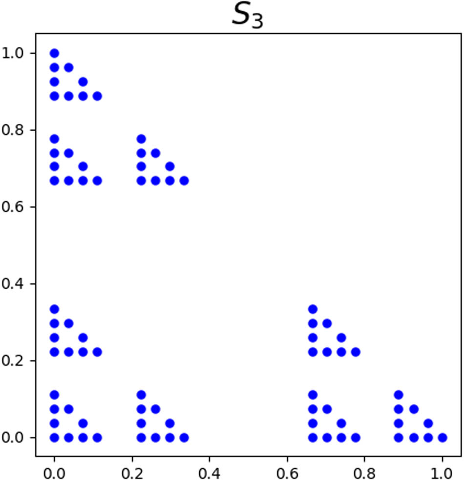
 { S n } n = 1 by S 1 = Ψ ( S 0 ) , and S n + 1 = Ψ ( S n ) for n N (Figure 5). Note that S n S n + 1 A for all n N and lim n d H ( S n , A ) = 0 . Let f n L ( N × R ) be the persistence landscape of H 0 Cěch ( S n ) . As before, lim n f n = f where f is the persistence landscape of H 0 Cěch ( A ) . Thus, we claim f n = f n + 1 .

Figure 5 
                  An illustration of 


                                    S
                                 
                                 
                                    3


                           {S}_{3}
                        
                      for the Cantor triangle.
Figure 5

An illustration of S 3 for the Cantor triangle.

Indeed, choose n N . Since diam ( A ) = 2 , it is clear that f n + 1 1 = τ ( 0 , 2 ) . For s t , let M s , t : H 0 Cěch ( S n , s ) H 0 Cěch ( S n , t ) and P s , t : H 0 Cěch ( S n + 1 , s ) H 0 Cěch ( S n + 1 , t ) denote the homomorphisms induced by the obvious inclusion mappings. Since Cěch ( S n + 1 , ε ) is path connected for ε 1 3 , this implies that rank H 0 Cěch ( S n + 1 , ε ) = 1 . On the other hand, for ε < 1 3 , we know that rank H 0 Cěch ( S n + 1 , ε ) 3 since Cěch ( S n + 1 , ε ) is not path connected, with ψ 1 ( S n ) , ψ 2 ( S n ) , ψ 3 ( S n ) S n + 1 each containing at least one distinct ε -component of S n + 1 . Therefore, for t R , j = 2 or j = 3 ,

f n + 1 ( j ) ( t ) = sup { m 0 rank P t m , t + m 3 } = max t , 1 3 = τ 0 , 1 3 ( t ) .

To compute f n + 1 ( j ) for j 4 , the key observation is that for 0 s t < 1 3 ,

(49) rank P s , t = 3 rank M 3 s , 3 t ,

and for s < 0 or t 1 3 , we obtain rank P s , t 1 . The second part is clear. To justify equation (49), note that for ε < 1 3 , since

min 1 j k 3 d ( ψ j ( S n ) , ψ k ( S n ) ) = 1 3 ,

and it follows from Lemma 2 that

H 0 Cěch ( S n + 1 , ε ) j = 1 3 H 0 Cěch ( S n , 3 ε ) .

Since every nontrivial transformation in H 0 Cěch ( S n ) and H 0 Cěch ( S n + 1 ) is a surjection, the previous isomorphism implies equation (49). If we assume j = 3 k + l for k N , and l { 1 , 2 , 3 } , then by definition,

(50) f n + 1 ( j ) ( t ) = sup { m 0 rank P t m , t + m j } = sup { m 0 3 rank M 3 ( t m ) , 3 ( t + m ) j } = sup { m 0 rank M 3 ( t m ) , 3 ( t + m ) k + 1 } .

On the other hand, for k N , we have

1 3 f n ( k + 1 ) ( 3 t ) = 1 3 sup { m 0 rank M 3 t m , 3 t + m k + 1 } = sup { m 3 0 rank M 3 t m , 3 t + m k + 1 } = sup { m 0 rank M 3 ( t m ) , 3 ( t + m ) k + 1 } = f n + 1 ( j ) ( t ) .

This proves the claim that f n = f n + 1 , meaning f = f .

When we compute the fixed point of by taking the limit lim n n 0 , we find that f = { f ( j ) } j = 1 , where

f ( j ) = τ ( 0 , 2 ) , if j = 1 , τ ( 0 , 3 1 ) , if 1 < j 3 , τ ( 0 , 3 k 1 ) , if 3 k < j 3 k + 1 for k N .

4.6 Distorted Sierpinksi Carpet

Consider another IFS on R 2 , Ψ = { ψ 1 , ψ 2 , ψ 3 , ψ 4 } , where

ψ 1 ( x , y ) = 1 3 I 2 ( x , y ) T , ψ 2 ( x , y ) = 1 3 I 2 [ ( x , y ) + ( 2 , 0 ) ] T , ψ 3 ( x , y ) = 1 3 I 2 [ ( x , y ) + ( 0 , 1 ) ] T , ψ 4 ( x , y ) = 1 3 I 2 [ ( x , y ) + ( 2 , 1 ) ] T .

A , the invariant set of Ψ , turns out to be C × 1 2 C . Clearly, Ψ does not have well-separated images since

min 1 j k 4 d ( ψ j ( A ) , ψ k ( A ) ) = 1 6 < 10 6 = diam ψ j ( A ) .

Even though we cannot apply Theorem 4 directly, we can derive the formula for f , the persistence landscape of H 0 Cěch ( A ) , using a similar argument to what we had in the previous section. We claim that : L ( N × R ) L ( N × R ) , defined by g = h , where

h ( 1 ) = τ 0 , 5 2 , h ( 2 ) = τ ( 0 , 1 3 ) , h ( 3 ) = h ( 4 ) = τ 0 , 1 6 , h ( 4 k + 1 ) ( t ) = h ( 4 k + 2 ) ( t ) = h ( 4 k + 3 ) ( t ) = h ( 4 k + 4 ) ( t ) = 1 3 g ( k + 1 ) ( 3 t ) for k N

satisfies f = f .

To prove this, we take S 0 = ( 0 , 0 ) , ( 1 , 0 ) , 0 , 1 2 , 1 , 1 2 and define a sequence of sets { S n } n = 1 , where

S 1 = Ψ ( S 0 ) , S n + 1 = Ψ ( S n ) for n N .

Let f n denote the persistence landscape function for S n , then we claim that satisfies f n = f n + 1 for all n N . Because lim n d H ( S n , A ) = 0 , it follows that lim n f n = f , and as we have reasoned in the previous examples, this implies that f = f .

To prove that f n = f n + 1 , fix n N . Since diam ( A ) = 5 2 , it is clear that f n + 1 1 = τ 0 , 5 2 . For s t , let M s , t : H 0 Cěch ( S n , s ) H 0 Cěch ( S n , t ) and P s , t : H 0 Cěch ( S n + 1 , s ) H 0 Cěch ( S n + 1 , t ) denote the homomorphisms induced by the obvious inclusion mappings. Since Cěch ( S n + 1 , ε ) is path connected for ε 1 3 , this implies that rank H 0 Cěch ( S n + 1 , ε ) = 1 . On the other hand, for ε [ 1 6 , 1 3 ) , we know that rank H 0 Cěch ( S n + 1 , ε ) = 2 since Cěch ( S n + 1 , ε ) is not path connected, with ψ 1 ( S n ) ψ 3 ( S n ) , ψ 2 ( S n ) ψ 4 ( S n ) S n + 1 each forming an ε -component of S n + 1 . For ε < 1 6 , we know that rank H 0 Cěch ( S n + 1 , ε ) 4 since

min 1 j 4 d ( ψ j ( S n ) , S n + 1 \ ψ j ( S n ) ) = 1 6 .

Therefore, for t R ,

f n + 1 ( 2 ) ( t ) = sup { m 0 rank P t m , t + m 2 } = max t , 1 3 t = τ 0 , 1 3 ( t ) ,

and for j = 3 , 4 ,

f n + 1 ( j ) ( t ) = sup { m 0 rank P t m , t + m 4 } = max t , 1 6 t = τ 0 , 1 6 ( t ) .

To compute f n + 1 ( j ) for j 5 , the key observation is that for 0 s t < 1 6 ,

(51) rank P s , t = 4 rank M 3 s , 3 t ,

and for s < 0 or t 16 , we obtain rank P s , t 2 . We have already established the second part. To justify equation (51), since ε < 1 6 implies that

min 1 j k 4 d ( ψ j ( S n ) , ψ k ( S n ) ) > ε ,

and it follows from Lemma 2 that

H 0 Cěch ( S n + 1 , ε ) j = 1 4 H 0 Cěch ( S n , 3 ε ) .

As in the previous example, this isomorphism implies (51). Using identical reasoning as in the previous section, this implies that for j = 4 k + l for k N and l { 1 , 2 , 3 , 4 } ,

f n + 1 ( j ) ( t ) = 1 3 f n ( k + 1 ) ( 3 t ) .

Thus, f n = f n + 1 for all n N . Therefore, f = f .

We compute the formula for f = { f ( j ) } j = 1 by taking the limit of n 0 as n . We find that

f ( j ) = τ 0 , 5 2 , if j = 1 , τ ( 0 , 3 1 ) , if j = 2 , τ ( 0 , 6 1 ) , if 2 < j 4 , τ ( 0 , 3 k 1 ) , if 4 k < j 2 4 k for k N , τ ( 0 , 3 k 6 1 ) , if 2 4 k < j 4 k + 1 k N .

In terms of equation (33), we have N = 4 , c = 1 3 , δ 1 = 5 2 , δ 2 = 1 3 , and δ 3 = δ 4 = 1 6 . This means the persistence landscape of H 0 Cěch ( A ) is consistent with the formula from Theorem 4 even though Ψ does not have well-separated images.

4.7 Remarks

The 1/5 Cantor set in 4.4 demonstrates how a reasonable formula for the persistence landscape of H 0 Cěch ( A ) can be found in the one-dimensional case, even when images are not well-separated. As long as the Cěch complex of the intersection of these images is reasonable, we can use the Mayer-Vietoris sequence to make precise the difference between rank H 0 Cěch ( Ψ ( S n ) , ε ) and what the rank would be if Ψ had well-separated images. The example also shows the intuition that each time two images are touching, we have to “skip” one of the first N terms in the sequence that makes up f .

The final two examples demonstrate that at least for zero-dimensional homology, the well-separated assumption can be too restrictive. We might be better off replacing the well-separated hypothesis with the assumption that

inf { ε > 0 C ( A , ε ) < N } max 1 j N inf { ε > 0 C ( ψ j ( A ) , ε ) = 1 } ,

since the proof of Theorem 4 seems to work as long each image becomes path connected by the time any two different images become path connected. However, the well-separated assumption might be necessary for finding the persistence landscape for H p Cěch ( A ) for p 1 . For p = 1 , it would guarantee that there are no loops persisting in individual images by the time loops could be “born” consisting of 1-chains consisting of a combination of different images.

  1. Funding information: Michael J. Catanzaro, Lee Przybylski, and Eric S. Weber were supported in part by the National Science Foundation under award #1934884. Lee Przybylski and Eric S. Weber were supported in part by the National Science Foundation and the National Geospatial Intelligence Agency under award #1830254.

  2. Author contributions: All authors have accepted responsibility for the entire content of this manuscript and approved its submission.

  3. Conflict of interest: Eric Weber is a member of the Editorial Board of Demonstratio Mathematica and was not involved in the review process of this article.

  4. Data availability statement: Code for generating persistence landscapes using pyscapes is available here: github.com/catanzaromj/PL_fractal. No other data were generated during the study.

References

[1] P. Bubenik, Statistical topological data analysis using persistence landscapes, J. Machine Learn. Res. 16 (2015), no. 1, 77–102. Search in Google Scholar

[2] V. Robins, Computational topology at multiple resolutions: foundations and applications to fractals and dynamics, Ph.D. thesis, University of Colorado, 2000. Search in Google Scholar

[3] G. Máté and D. W. Heermann, Persistence intervals of fractals, Phys. A Statist. Mech. Appl. 405 (2014), 252–259. 10.1016/j.physa.2014.03.037Search in Google Scholar

[4] G. Carlsson, A. Zomorodian, A. Collins, and L. J. Guibas, Persistence barcodes for shapes, Int. J. Shape Model. 11 (2005), no. 2, 149–187. 10.1145/1057432.1057449Search in Google Scholar

[5] E. Munch, K. Turner, P. Bendich, S. Mukherjee, J. Mattingly, and J. Harer, Probabilistic Fréchet means for time varying persistence diagrams, Electron. J. Statistic. 9 (2015), no. 1, 1173–1204. 10.1214/15-EJS1030Search in Google Scholar

[6] V. Kovacev-Nikolic, P. Bubenik, D. Nikolic, and G. Heo, Using persistent homology and dynamical distances to analyze protein binding, Statistic. Appl. Genetics Mol. Biol. 15 (2016), no. 1, 19–38. 10.1515/sagmb-2015-0057Search in Google Scholar PubMed

[7] I. Donato, M. Gori, M. Pettini, G. Petri, S. De Nigris, R. Franzosi, et al., Persistent homology analysis of phase transitions, Phys. Rev. E 93 (2016), no. 5, 052138. 10.1103/PhysRevE.93.052138Search in Google Scholar PubMed

[8] J.-Y. Liu, S.-K. Jeng, and Y.-H. Yang, Applying topological persistence in convolutional neural network for music audio signals, 2016, arXiv: http://arXiv.org/abs/arXiv:1608.07373. Search in Google Scholar

[9] P. Dlotko and T. Wanner, Topological microstructure analysis using persistence landscapes, Phys. D 334 (2016), 60–81. 10.1016/j.physd.2016.04.015Search in Google Scholar

[10] G. Cantor, De la puissance des ensembles parfaits de points, Acta Math. 4 (1884), no. 1, 381–392. 10.1007/BF02418423Search in Google Scholar

[11] R. S. Strichartz, Analysis on fractals, Notices Amer. Math. Soc. 46 (1999), no. 10, 1199–1208. Search in Google Scholar

[12] J. W. S. Cassels, On a problem of Steinhaus about normal numbers, Colloq. Math. 7 (1959), 95–101. 10.4064/cm-7-1-95-101Search in Google Scholar

[13] W. M. Schmidt, Über die Normalität von Zahlen zu verschiedenen Basen, Acta Arith. 7 (1961/1962), 299–309. 10.4064/aa-7-3-299-309Search in Google Scholar

[14] R. Lyons and Y. Peres, Probability on Trees and Networks, Cambridge Series in Statistical and Probabilistic Mathematics, Cambridge University Press, New York, 2017. 10.1017/9781316672815Search in Google Scholar

[15] P. E. T. Jorgensen, Analysis and Probability: Wavelets, Signals, Fractals, Graduate Texts in Mathematics, vol. 234, Springer, New York, 2006. Search in Google Scholar

[16] A. Byars, E. Camrud, S. N. Harding, S. McCarty, K. Sullivan, and E. S. Weber, Sampling and interpolation of cumulative distribution functions of Cantor sets in [0, 1], Dem. Math. 54 (2021), 85–109. 10.1515/dema-2021-0010Search in Google Scholar

[17] A. D. Pollington, The Hausdorff dimension of a set of normal numbers. II, J. Austral. Math. Soc. Ser. A 44 (1988), no. 2, 259–264. 10.1017/S1446788700029840Search in Google Scholar

[18] Y. Peres and B. Solomyak, Self-similar measures and intersections of Cantor sets, Trans. Amer. Math. Soc. 350 (1998), no. 10, 4065–4087. 10.1090/S0002-9947-98-02292-2Search in Google Scholar

[19] C. Allain and M. Cloitre, Characterizing the lacunarity of random and deterministic fractal sets, Phys. Rev. A 44 (1991), 3552–3558. 10.1103/PhysRevA.44.3552Search in Google Scholar PubMed

[20] B. Yu, M. Zou, and Y. Feng, Permeability of fractal porous media by Monte Carlo simulations, Int. J. Heat Mass Transf. 48 (2005), 2787–2794. 10.1016/j.ijheatmasstransfer.2005.02.008Search in Google Scholar

[21] B. Yu, Fractal dimensions for multiphase fractal media, Fractals 14 (2006), no. 2, 111–118. 10.1142/S0218348X06003155Search in Google Scholar

[22] P. E. T. Jorgensen and Steen Pedersen, Dense analytic subspaces in fractal L2-spaces, J. Anal. Math. 75 (1998), 185–228. 10.1007/BF02788699Search in Google Scholar

[23] R. S. Strichartz, Mock Fourier series and transforms associated with certain Cantor measures, J. Anal. Math. 81 (2000), 209–238. 10.1007/BF02788990Search in Google Scholar

[24] R. J. Ravier and R. S. Strichartz, Sampling theory with average values on the Sierpinski gasket, Constr. Approx. 44 (2016), no. 2, 159–194. 10.1007/s00365-016-9341-7Search in Google Scholar

[25] J. E. Hutchinson, Fractals and self similarity, Indiana Univ. Math. J. 30 (1981), no. 5, 713–747. 10.1512/iumj.1981.30.30055Search in Google Scholar

[26] A. Hatcher, Algebraic Topology, Cambridge University Press, Cambridge, 2002. Search in Google Scholar

[27] J. R Munkres, Elements of Algebraic Topology, Addison-Wesley Publishing Company, Boston, Massachusetts, United States, 1984. Search in Google Scholar

[28] H. Edelsbrunner and J. Harer, Computational Topology: An Introduction, American Mathematical Society, Providence, RI 2010. 10.1090/mbk/069Search in Google Scholar

[29] J. A. Perea, A brief history of persistence, 2018, arXiv:1809.03624 [cs, math]. Search in Google Scholar

[30] K. Borsuk, On the imbedding of systems of compacta in simplicial complexes, Fundamenta Math. 35 (1948), 217–234 (eng). 10.4064/fm-35-1-217-234Search in Google Scholar

[31] U. Bauer, Ripser: efficient computation of Vietoris–Rips persistence barcodes, J. Appl. Comput. Topology 5 (2021), no. 5, 391–423, DOI: https://doi.org/10.1007/s41468-021-00071-5.10.1007/s41468-021-00071-5Search in Google Scholar

[32] V. De Silva and R. Ghrist, Coverage in sensor networks via persistent homology, Algebraic Geometric Topol. 7 (2007), no. 1, 339–358. 10.2140/agt.2007.7.339Search in Google Scholar

[33] M. Bakke Botnan and W. Crawley-Boevey, Decomposition of persistence modules, Proc. Amer. Math. Soc. 148 (2020), 4581–4596, DOI: https://doi.org/10.1090/proc/14790.10.1090/proc/14790Search in Google Scholar

[34] G. Azumaya, Corrections and supplementaries to my paper concerning Krull-Remak-Schmidt’s theorem, Nagoya Math. J. 1 (1950), 117–124 (eng). 10.1017/S002776300002290XSearch in Google Scholar

[35] F. Chazal, V. de Silva, M. Glisse, and S. Oudot, The structure and stability of persistence modules, Springer Briefs in Mathematics, Springer, Cham, 2016. 10.1007/978-3-319-42545-0Search in Google Scholar

[36] F. Chazal, D. Cohen-Steiner, M. Glisse, L. J. Guibas, and S. Oudot, Proximity of persistence modules and their diagrams, Research report RR-6568, INRIA, 2008. 10.1145/1542362.1542407Search in Google Scholar

[37] D. Cohen-Steiner, H. Edelsbrunner, and J. Harer, Stability of persistence diagrams, Discrete Comput. Geometry 37 (2007), no. 1, 103–120. 10.1145/1064092.1064133Search in Google Scholar

[38] F. Chazal, V. de Silva, and S. Oudot, Persistence stability for geometric complexes, Geom. Dedicata 173 (2014), 193–214. 10.1007/s10711-013-9937-zSearch in Google Scholar

[39] P. Bubenik, The persistence landscape and some of its properties, Topological Data Analysis, Abel Symposia, Springer International Publishing, Cham, 2020, pp. 97–117 (eng). 10.1007/978-3-030-43408-3_4Search in Google Scholar

[40] G. Angeloro and M. J. Catanzaro, Pyscapes (version 0.1.0), https://github.com/gabbyangeloro/pyscapes. Search in Google Scholar

Received: 2022-01-05
Revised: 2022-03-29
Accepted: 2022-04-25
Published Online: 2022-05-27

© 2022 Michael J. Catanzaro et al., published by De Gruyter

This work is licensed under the Creative Commons Attribution 4.0 International License.

Articles in the same Issue

  1. Regular Articles
  2. On some summation formulas
  3. A study of a meromorphic perturbation of the sine family
  4. Asymptotic behavior of even-order noncanonical neutral differential equations
  5. Unconditionally positive NSFD and classical finite difference schemes for biofilm formation on medical implant using Allen-Cahn equation
  6. Starlike and convexity properties of q-Bessel-Struve functions
  7. Mathematical modeling and optimal control of the impact of rumors on the banking crisis
  8. On linear chaos in function spaces
  9. Convergence of generalized sampling series in weighted spaces
  10. Persistence landscapes of affine fractals
  11. Inertial iterative method with self-adaptive step size for finite family of split monotone variational inclusion and fixed point problems in Banach spaces
  12. Various notions of module amenability on weighted semigroup algebras
  13. Regularity and normality in hereditary bi m-spaces
  14. On a first-order differential system with initial and nonlocal boundary conditions
  15. On solving pseudomonotone equilibrium problems via two new extragradient-type methods under convex constraints
  16. Local linear approach: Conditional density estimate for functional and censored data
  17. Some properties of graded generalized 2-absorbing submodules
  18. Eigenvalue inclusion sets for linear response eigenvalue problems
  19. Some integral inequalities for generalized left and right log convex interval-valued functions based upon the pseudo-order relation
  20. More properties of generalized open sets in generalized topological spaces
  21. An extragradient inertial algorithm for solving split fixed-point problems of demicontractive mappings, with equilibrium and variational inequality problems
  22. An accurate and efficient local one-dimensional method for the 3D acoustic wave equation
  23. On a weighted elliptic equation of N-Kirchhoff type with double exponential growth
  24. On split feasibility problem for finite families of equilibrium and fixed point problems in Banach spaces
  25. Entire and meromorphic solutions for systems of the differential difference equations
  26. Multiplication operators on the Banach algebra of bounded Φ-variation functions on compact subsets of ℂ
  27. Mannheim curves and their partner curves in Minkowski 3-space E13
  28. Characterizations of the group invertibility of a matrix revisited
  29. Iterates of q-Bernstein operators on triangular domain with all curved sides
  30. Data analysis-based time series forecast for managing household electricity consumption
  31. A robust study of the transmission dynamics of zoonotic infection through non-integer derivative
  32. A Dai-Liao-type projection method for monotone nonlinear equations and signal processing
  33. Review Article
  34. Remarks on some variants of minimal point theorem and Ekeland variational principle with applications
  35. Special Issue on Recent Methods in Approximation Theory - Part I
  36. Coupled fixed point theorems under new coupled implicit relation in Hilbert spaces
  37. Approximation of integrable functions by general linear matrix operators of their Fourier series
  38. Sharp sufficient condition for the convergence of greedy expansions with errors in coefficient computation
  39. Approximation of conic sections by weighted Lupaş post-quantum Bézier curves
  40. On the generalized growth and approximation of entire solutions of certain elliptic partial differential equation
  41. Existence results for ABC-fractional BVP via new fixed point results of F-Lipschitzian mappings
  42. Linear barycentric rational collocation method for solving biharmonic equation
  43. A note on the convergence of Phillips operators by the sequence of functions via q-calculus
  44. Taylor’s series expansions for real powers of two functions containing squares of inverse cosine function, closed-form formula for specific partial Bell polynomials, and series representations for real powers of Pi
  45. Special Issue on Recent Advances in Fractional Calculus and Nonlinear Fractional Evaluation Equations - Part I
  46. Positive solutions for fractional differential equation at resonance under integral boundary conditions
  47. Source term model for elasticity system with nonlinear dissipative term in a thin domain
  48. A numerical study of anomalous electro-diffusion cells in cable sense with a non-singular kernel
  49. On Opial-type inequality for a generalized fractional integral operator
  50. Special Issue on Advances in Integral Transforms and Analysis of Differential Equations with Applications
  51. Mathematical analysis of a MERS-Cov coronavirus model
  52. Rapid exponential stabilization of nonlinear continuous systems via event-triggered impulsive control
  53. Novel soliton solutions for the fractional three-wave resonant interaction equations
  54. The multistep Laplace optimized decomposition method for solving fractional-order coronavirus disease model (COVID-19) via the Caputo fractional approach
  55. Special Issue on Problems, Methods and Applications of Nonlinear Analysis
  56. Some recent results on singular p-Laplacian equations
  57. Infinitely many solutions for quasilinear Schrödinger equations with sign-changing nonlinearity without the aid of 4-superlinear at infinity
  58. Special Issue on Recent Advances for Computational and Mathematical Methods in Scientific Problems
  59. Existence of solutions for a nonlinear problem at resonance
  60. Asymptotic stability of solutions for a diffusive epidemic model
  61. Special Issue on Computational and Numerical Methods for Special Functions - Part I
  62. Fully degenerate Bernoulli numbers and polynomials
  63. Wigner-Ville distribution and ambiguity function associated with the quaternion offset linear canonical transform
  64. Some identities related to degenerate Stirling numbers of the second kind
  65. Two identities and closed-form formulas for the Bernoulli numbers in terms of central factorial numbers of the second kind
  66. λ-q-Sheffer sequence and its applications
  67. Special Issue on Fixed Point Theory and Applications to Various Differential/Integral Equations - Part I
  68. General decay for a nonlinear pseudo-parabolic equation with viscoelastic term
  69. Generalized common fixed point theorem for generalized hybrid mappings in Hilbert spaces
  70. Computation of solution of integral equations via fixed point results
  71. Characterizations of quasi-metric and G-metric completeness involving w-distances and fixed points
  72. Notes on continuity result for conformable diffusion equation on the sphere: The linear case
Downloaded on 14.9.2025 from https://www.degruyterbrill.com/document/doi/10.1515/dema-2022-0015/html
Scroll to top button