Influence of propeller shaft angles on the speed performance of composite fishing boats
-
Pham-Thanh Nhut


Abstract
The propeller shaft inclination angle is one of the critical parameters influencing the speed of a fishing boat. This study assesses how the propeller shaft inclination angle impacts the speed of composite fishing boats through experimental and numerical analyses. The model used for testing is a scaled-down version of a 24.0 m × 6.5 m × 3.5 m fishing boat, constructed at a 1:12 scale using composite materials (polyester resin and fiberglass). The model allows for the propeller shaft angle adjustment from 0° to 15°. The model was tested at the design speed of 2.9 knots to measure the vessel’s speed corresponding to various inclination angles. Additional tests were conducted at lower (2.31 knots) and higher (3.46 knots) speeds to validate the results. The model was also simulated using computational fluid dynamics (CFD) software to compare and assess the reliability of the experimental results. Subsequently, the CFD software was employed to simulate the actual vessel and evaluate its performance. The results of the experiments and simulations demonstrate significant variations in vessel speed as the inclination angle increases from 0° to 15°. The maximum speed was achieved when the propeller shaft inclination angle ranged between 6° and 7° (reaching 3.05 knots). The vessel speed decreased substantially when the inclination angle increased from 9° to 15°. The speed variation patterns for the 2.31 knot and 2.9 knot cases were similar, whereas the 3.46 knot case exhibited notable differences. The optimal propeller shaft inclination angle range for achieving high speeds for the studied vessel lies between 3° and 8°.
1 Introduction
The vessel’s speed depends on many factors, including resistance, main engine power, characteristics of the shaft system, propeller, and installation technologies. Research on resistance is a top priority among others, with many studies and publications addressing this issue. However, the hydrodynamic problem affecting the ship’s hull remains highly complex and has yet to be satisfactorily resolved. In addition to hull resistance, the propeller shaft inclination angle has garnered significant attention, as it is one of the critical parameters impacting the vessel’s speed. However, research on the propeller shaft inclination angle, especially for fishing boats, is limited.
Theoretically, no literature has addressed the propeller shaft inclination angle parameter in the context of speed or resistance calculations for fishing vessels. Specialized software for evaluating the performance of fishing vessels also does not require input data regarding the propeller shaft inclination angle or related parameters. Meanwhile, determining the propeller shaft inclination angle for wooden and composite fishing vessels is primarily based on empirical experiences. Although composite fishing vessels have been systematically designed and constructed based on established theory, the issue of determining the optimal propeller shaft inclination angle remains unresolved. Therefore, finding a reasonable inclination angle to optimize vessel speed is both necessary and feasible, primarily through experimental research. However, conducting experiments on actual vessels is prohibitively expensive and almost impractical. Thus, this study investigates the influence of the propeller shaft inclination angle on composite fishing vessels through experimental modeling.
One of the critical factors affecting ship speed, especially in fishing vessels, is the angle of the propeller shaft inclination. However, there has been little research on ships’ propeller shaft inclination angle, especially fishing vessels. For this, some of the previous studies for fishing vessels or low-speed ships, such as the work by Santoso et al. [1], study the effect of central engine position and the propeller shaft inclination angle on vessel performance using numerical simulation methods. They conducted the study in a 60 GT fishing vessel with a design length of 21.98 m, as shown in Figure 1. Two primary engine locations were investigated: 4.0–6.5 m and 5.5–8.0 m from the aft bulkhead. The shaft inclination angle of the propeller was kept in a range of 1.0°–4.0° for each engine position. Results from the simulations were compared against calculations from the Maxsurf software (using the Oortmerssen and Holtrop methods) and experimental data. The results showed that installing the main engine closer to the aft bulkhead is ideal with less resistance. In this configuration, the resistance decreased mildly from 1.0° to 4.0° for the propeller shaft inclination angle.
![Figure 1
Fishing vessel models provided by Santoso et al. [1].](/document/doi/10.1515/cls-2025-0032/asset/graphic/j_cls-2025-0032_fig_001.jpg)
Fishing vessel models provided by Santoso et al. [1].
Van [2] studied the motion dynamics of fire-fighting boats for Melaleuca forest fires. The research subject was a fire-fighting boat with a maximum length of 4.26 m, equipped with a primary engine of 15 kW, as indicated in Figure 2. The study employed experimental methods to determine the boat’s speed corresponding to different propeller shaft inclination angles. The results showed that when the propeller shaft inclination angle was varied from 5° to 25°, the maximum speed was achieved at an inclination angle of 20°.
![Figure 2
Fire-fighting boat model [2] (1 – main engine; 2 – fixed water pump; 3 – portable water pump).](/document/doi/10.1515/cls-2025-0032/asset/graphic/j_cls-2025-0032_fig_002.jpg)
Fire-fighting boat model [2] (1 – main engine; 2 – fixed water pump; 3 – portable water pump).
The propeller shaft inclination angle for planning high-speed vessels has been studied. However, there is a new method to calculate the hydrodynamics of planing vessels by Savitsky [3], including flat (the angle between the thrust line of the propeller and the baseline) and draft (the angle between the baseline and the vessel’s draft), as described in Figure 3. This approach was validated using experimental data collected at Davidson Laboratory. This experiment was performed on a symmetrical deadrise hull design. Measurements, including the coefficient of friction on flat plates, were also tested. The Savitsky method, initially proposed in 1964, has been further developed and widely adopted in the design of planning vessels [3]. These advances have allowed it to be applied to vessel design. Several researchers have utilized the approach to estimate the parameters of a planning vessel and compare results with experimental data, as well as computational fluid dynamics (CFD) simulations. Thus, the Savitsky method is widely used to calculate the hydrodynamic components of planning vessels.
![Figure 3
Hydrodynamic components of planing vessels by Savitsky [3].](/document/doi/10.1515/cls-2025-0032/asset/graphic/j_cls-2025-0032_fig_003.jpg)
Hydrodynamic components of planing vessels by Savitsky [3].
Bate [4] conducted the analysis and prediction of high-speed vessel performance. In this work, the author utilized a mathematical model to analyze the hydrodynamic characteristics of monohull high-speed vessels. Based on these results, the author evaluated vessel performance under different operating conditions, providing a basis for potential application to trimaran vessels. Skupień and Prokopowicz [5] investigated several methods for calculating the resistance of inland waterway vessels. These methods were validated for different types of boats and varying conditions using the results of model tests. According to this study, the vessel’s shape parameters and draft were adjusted during the experiments to determine vessel speed and fuel consumption. The operation manual of DOOSAN marine engines [6] specifies the permissible inclination angles for main engine installation (Figure 4). Depending on the engine model, the allowable inclination angles range from a minimum of 17° to a maximum of 30°.
![Figure 4
Permissible inclination angles for DOOSAN main engine installation [6].](/document/doi/10.1515/cls-2025-0032/asset/graphic/j_cls-2025-0032_fig_004.jpg)
Permissible inclination angles for DOOSAN main engine installation [6].
Hien [7] studied the application of CFD theory in calculating the resistance of a high-speed composite-hull vessel. Daniel Savitsky’s theory was used to estimate the resistance of two models of high-speed vessels developed and built by the Shipbuilding Research and Manufacturing Institute. These include concepts like the angle of inclination between the propeller thrust line and the reference line and the angle between the reference line and the vessel’s draft. Experimental investigations of the effects of immersion ratio and shaft inclination angle on surface-piercing propeller performance were also reported by Seyyedi et al. [8]. The test object was a five-blade surface-piercing propeller in a free-surface water tunnel. The study analyzed the effects of immersion ratio and shaft inclination angle on the propeller efficiency and hydrodynamic coefficients. The findings showed that the thrust and torque hydrodynamic coefficients were positively related to the immersion ratio, while the hydrodynamic thrust coefficient and efficiency were inversely related. The torque coefficient was also raised with a larger angle of attack on the shafts. An immersion ratio of 40–50% was shown to produce the maximum propeller efficiency at all shaft inclination angles. The highest degree of efficiency was obtained at zero shaft inclination angle, whereas the lowest was achieved at the 15° inclination angle of the shaft for all immersion ratios. The ideal propeller performance obtained was at a 50% immersion ratio and zero shaft inclination angle.
Beyond the research about the angle inclination of propeller shafts in ships, in some works like the references sleeping in the mythology vehicles of the instigation, the theory of similarity of the ship model is very much in portals by Birk [10], and Duc-An and Ban [11]. Based on these reference studies in scaled-down ship models, the similarities of still water line, hull speed up, and scalene properties must comply with laws of geometry or geometric, kinematics, and dynamics similarity. Meanwhile, many articles have been published regarding the all-scaled ship resistance test with model ships. Among those, Ngoc-Tu et al. [12] studied the effect of the scale of the model on the variation of flow characteristics around the hull using the CFD methods. Qualitative differences between model and full-scale ships were identified and examined, including wave patterns produced by the moving boat, dynamic pressure distribution, shear stress on the hull surface, and wake flow. The reliability of the simulations was verified by comparing the simulation results against the experimental data. Hetharia et al. [13] observed differences between estimates of engine power gained in the early planning stages and those obtained using the available model testing methods. They found discrepancies between computational results and lab testing findings in fishing boats, passenger-cargo ships, and semi-displacement boats. Zhang et al. [14] proposed an energy efficiency performance model developed explicitly for inland waterway vessels. The power determination is based on high-precision model testing and simulation. The results showed that the experimental methods provided a very accurate knowledge of the vessel’s power needs.
Thi-Ha-Phuong and Thi-Hai-Ha [15] predicted the resistance of a tanker model compared to a full-scale ship using CFD methods. This study was performed on a model of a tanker vessel cruising steadily through calm water using numerical simulations with the STAR-CCM + software. The Reynolds-averaged Navier–Stokes (RANS) equations were solved to simulate the flow field around the hull. The total resistance of the ship was then compared to published results from tank model tests. Overall, the high reliability of the STAR-CCM + software and the numerical method used for resistance simulation in static water through ship-scale models is evidenced by the results, with an error margin of less than 3.0%. There are also significant studies on Vietnamese fishing resistance, such as those noted by Le and Dinh-Tu [16], which include propellers and rudders around fishing vessel hulls. The authors used CFD simulations, mainly utilizing two tools, OrCA3D Marine CFD and Simerics. The results showed that at an operational speed of 10 knots, the hull resistance increased by 13.95, 9.5, and 7.53% for three loading conditions with drafts of d = 1.848, 1.53, and 1.323 m, respectively, compared to cases ignoring the effects of propeller and rudder. The velocity and pressure distribution in the stern region indicated an important difference in the presence and absence of the propeller and rudder. Higher saw that in the velocity distribution vector diagrams, the stern’s wake region tended to diminish, which was influenced by the propellant.
The analysis of the previous studies reveals the following findings: (1) studies on the propeller shaft inclination angle include theoretical, experimental, and simulation studies; (2) theoretical calculations are mainly conducted for high-speed vessels and planning boats; and (3) the propeller shaft inclination angle has been analyzed in fishing vessels. However, most studies are only focused on numerical simulation with limited inclination angles. It indicates that the shaft inclination parameters are not the subject of considerable research concerning ship resistance and speed. Therefore, this article experimentally models and numerical analyses the impact of propeller shaft inclination angle on a composite fishing boat.
2 Methodology
In order to investigate the effect of propeller shaft inclination angle on the fishing vessel speed, the selected case study of research is a composite fishing boat. The reference vessel has an overall length of 24.0 m, a width of 6.5 m, and a height of 3.5 m. To allow the propeller shaft inclination angle from 0° to 15° to the vessel hull, a 1:12 scale model was designed and fabricated. The model was tested at the design speed of 2.9 knots, and supplementary tests were conducted at lower (2.31 knots) and higher (3.46 knots) speeds. Numerical simulations (CFD) for the model and full-scale vessels were also conducted to assess the validity of the experimental results.
2.1 Target structure
Based on the environmental categories of interest, a vessel type with a maximum length of 24 m that can perform both purse seining and gillnetting has been chosen. More than 40 units of this model have been constructed and are actively used by fishermen in various economies. The summary of the main specifications of the vessel is presented in Table 1. The selected vessel type has the following characteristics:
It must be class-approved by a recognized design classification society.
The vessel must be built according to the approved design and capable of operating under relevant conditions.
It should be a popular choice for a fishing boat, considering both operational aspects and efficiency.
The vessel type must be evaluated by experienced fishermen.
Main specifications of the composite fishing boat
| Specifications | Symbol | Unit | Value |
|---|---|---|---|
| Length overall | L oa | m | 24.00 |
| Design length | L d | m | 21.36 |
| Breadth | B | m | 6.50 |
| Design breadth | B d | m | 6.09 |
| Depth | D | m | 3.50 |
| Design draft | T d | m | 1.93 |
| Displacement | Δ | ton | 184.70 |
| Block coefficient | Cb | — | 0.72 |
| Main engine power | NeS | HP | 800 |
| Speed | V S | knot | 10 |
| Commercial fishing | — | — | Purse seine fishermen |
| Operating area of the vessel | — | — | Restricted operating area I |
| Material | — | — | Composite |
It must have a sufficient stern area to allow for propeller clearance and the ability to adjust the inclination angle of the shaft.
Based on the actual dimensions of the prototype composite fishing vessel, the model vessel was selected with a scaling ratio of 1:12 compared to the actual vessel. The detailed specifications are presented in Table 2. In this table, the design speed of the model is calculated using the following Eq. (1) [9]:
where V s is the design speed of the actual fishing boat (m), V m is the design speed of the scaled model fishing boat (m), L s is the length of the actual fishing boat (m), and L m is the length of the scaled model fishing boat (m).
Main specifications of the scaled composite fishing boat model
| Specifications | Symbol | Unit | Value |
|---|---|---|---|
| Length overall | L oa | m | 2.00 |
| Design length | L d | m | 1.78 |
| Breadth | B | m | 0.54 |
| Design breadth | B d | m | 0.51 |
| Depth | D | m | 0.29 |
| Design draft | T d | m | 0.16 |
| Displacement | Δ | kg | 107.19 |
| Block coefficient | C b | — | 0.72 |
| Main engine power | NeS | HP | 0.80 |
| Main engine revolutions | n e | RPM | 7,000 |
| Gear ratio | i | — | 1:2.5 |
| Design speed | V m | knot | 2.90 |
| Material | — | — | Composite |
The model vessel is constructed using fiberglass composite material and polyester resin. The main engine used is a two-stroke, single-cylinder gasoline engine. To ensure that the model’s speed exceeds the design speed by approximately 30%, this margin is applied to account for potential increases in resistance or power loss due to installation inaccuracies. At the design speed (2.9 knots), the main engine power is determined by calculating the vessel’s resistance. This study uses two methods to calculate the model vessel’s resistance: the Holtrop method [17,18] and the Van Oortmerssen method [19]. Holtrop [17] and Holtrop and Mennen [18] have also developed an empirical method for estimating the resistance and engine power of the ship based on regression data from both model tests and full-scale ships, and it is widely adopted in practice. It predicts total resistance and required power, taking into account a range of hull form parameters and operational conditions. Another method for predicting power was proposed by Van Oortmerssen [19], which is based on mathematical models that incorporate ship geometry, Froude number, Reynolds number, and the propeller characteristics. This approach is beneficial for small ships and fishing boats. The results of the resistance calculations are presented in Table 3 and Figure 5.
Resistance calculations for the model fishing vessel
| Speed (knots) | Holtrop | Van Oortmerssen | ||
|---|---|---|---|---|
| Resistance (N) | Engine power (10−3 HP) | Resistance (N) | Engine power (10−3 HP) | |
| 0 | 0 | 0 | 0 | 0 |
| 0.125 | 0.077 | 0.007 | 0.025 | 0.002 |
| 0.250 | 0.288 | 0.050 | 0.083 | 0.014 |
| 0.375 | 0.624 | 0.161 | 0.169 | 0.044 |
| 0.500 | 1.080 | 0.373 | 0.280 | 0.097 |
| 0.625 | 1.654 | 0.713 | 0.417 | 0.180 |
| 0.750 | 2.341 | 1.211 | 0.577 | 0.299 |
| 0.875 | 3.140 | 1.896 | 0.760 | 0.459 |
| 1.000 | 4.063 | 2.803 | 0.966 | 0.666 |
| 1.125 | 5.145 | 3.993 | 1.193 | 0.926 |
| 1.250 | 6.467 | 5.576 | 1.442 | 1.243 |
| 1.375 | 8.172 | 7.752 | 1.712 | 1.624 |
| 1.500 | 10.476 | 10.841 | 2.002 | 2.072 |
| 1.625 | 13.657 | 15.311 | 2.314 | 2.594 |
| 1.750 | 18.040 | 21.780 | 2.645 | 3.193 |
| 1.875 | 23.950 | 30.980 | 2.996 | 3.876 |
| 2.000 | 31.663 | 43.687 | 3.368 | 4.646 |
| 2.125 | 41.365 | 60.640 | 3.758 | 5.510 |
| 2.250 | 53.141 | 82.487 | 4.169 | 6.471 |
| 2.375 | 67.000 | 109.777 | 4.598 | 7.534 |
| 2.500 | 82.900 | 142.978 | 5.047 | 8.704 |
| 2.625 | 100.787 | 182.518 | 5.514 | 9.986 |
| 2.750 | 120.606 | 228.810 | 6.001 | 11.384 |
| 2.875 | 142.317 | 282.272 | 6.506 | 12.903 |
| 2.900 | 148.036 | 296.808 | 6.635 | 13.303 |
| 3.000 | 165.890 | 343.334 | 7.029 | 14.548 |
| 3.125 | 191. 308 | 412.438 | 7.571 | 16.323 |
| 3.250 | 218.558 | 490.032 | 8.132 | 18.233 |
| 3.375 | 252.682 | 574.244 | 8.711 | 20.281 |
| 3.500 | 292.421 | 652.544 | 9.307 | 22.473 |
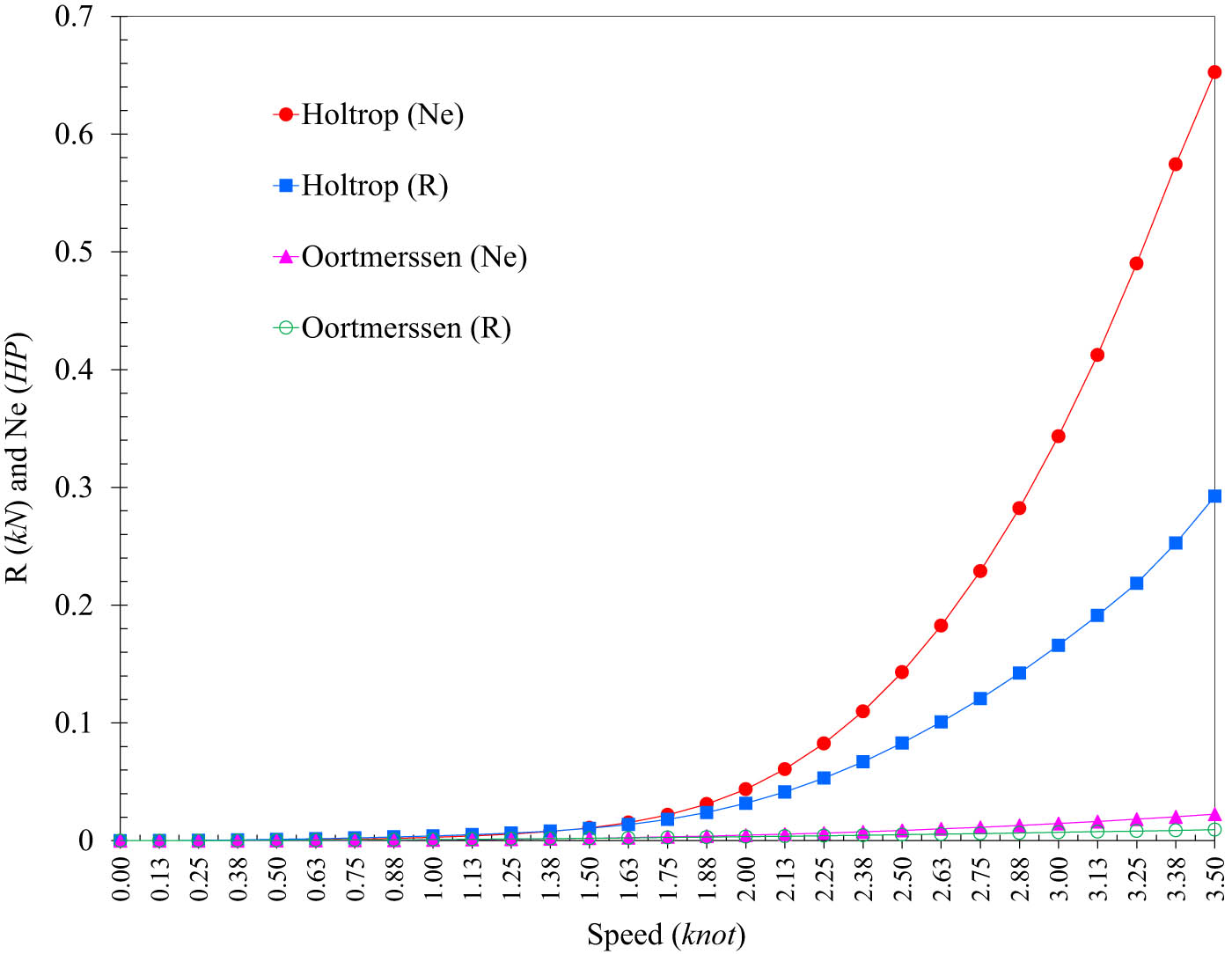
Resistance calculation results of the scaled composite fishing boat model.
When calculating the resistance of the actual vessel at a speed of 10 knots, the main engine power estimated using the Holtrop method is 750.99 HP. In contrast, the Van Oortmerssen method estimates it at 1582.01 HP. The Holtrop method provides a power estimation closer to the actual vessel’s main engine power (800 HP) than the Van Oortmerssen method. Therefore, the Holtrop method was selected to calculate the scaled model vessel’s resistance and main engine power. According to this method, at a speed of 2.9 knots, the model’s resistance is 148.036 N, and the main engine power is 0.3 HP. Based on the requirements for selecting the main engine, an engine with 0.8 HP and 7,000 RPM (Revolutions Per Minute) was chosen for the model. With this engine, the model can achieve a maximum speed of up to 3.77 knots (exceeding the design speed by approximately 30%). The model vessel is remotely controlled, and the control system components ensure stable operation with a maximum distance of up to 200 m between the controller and the vessel.
2.2 Model fabrication
The scaled model vessel was fabricated to replicate the general design and dimensions of the actual fishing boat. The 1:12 scale model of the vehicle was built to maintain geometric, kinematic, and dynamic similarity to the actual ship. Due to their lightweight, durable, and easy access to small-scale models, fiberglass composite and polyester resin were selected as the primary material type [20,21]. A flowchart of the scaled model fabrication process is described in Figure 6.
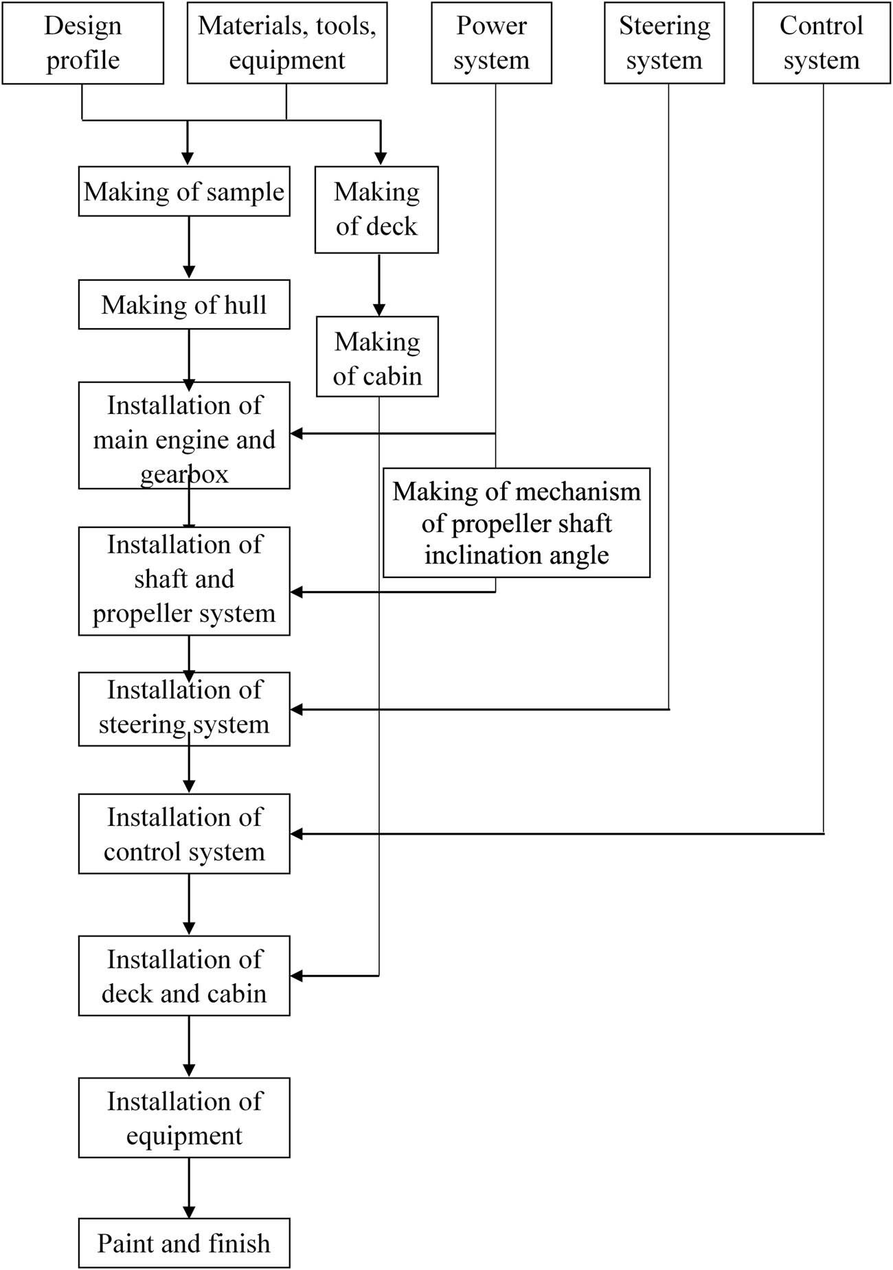
Flowchart of the scaled model fabrication process.
The model was fabricated by first scaling down the hull geometry from the drawings of the actual vessel. Formex sheets were used to print longitudinal and transverse cross-sections of the hull, which were then cut up into parts. The structural skeleton of the model was assembled from these parts with the help of some adhesive. The hull was upheld with a 3 mm-thick Formex sheet without sacrificing shape. After that, the hull was coated with polyester resin and 3–4 layers of 300 g/m2 fiberglass mat at the targeted hull thickness. Once the composite had cured for 48 h, they progressively sanded the hull surface from sandpapers 60, 120, 300, and 600 grit to get a well-sanded and actual surface. The depressions were filled with putty, and the surfaces were finally adjusted to the molding specifications of the hull shape. The two-color hull and waterline are marked clearly; brown is below the mark, and blue is above it. The deck and the cabin were stitched together from Formex over the hull, as shown in Figure 7.
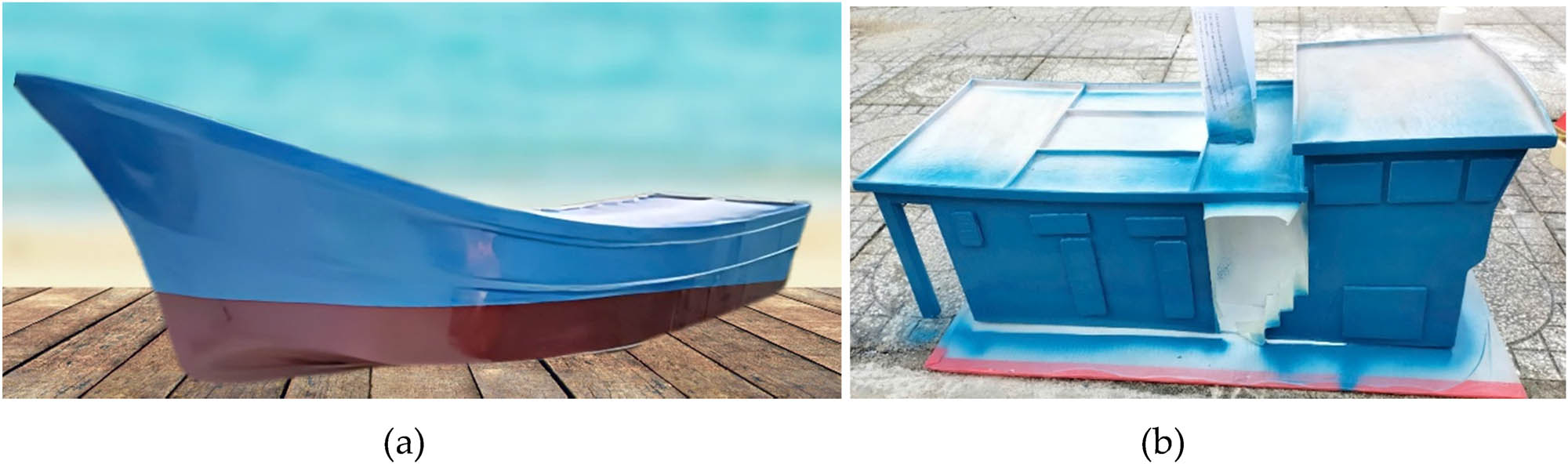
Fabrication of the model hull: (a) hull and (b) cabin.
The propulsion consisted of a 0.8 HP, 7,000 RPM gasoline engine fixed on a sturdy base and bolted to the hull. Two of the excitement came in the form of a gearbox and fuel tank; a bilge pump and battery were installed to power ancillary systems (Figure 8a). The most central feature of the model was the implementation and installation of the mechanism, which was able to change the angle of inclination of the propeller shaft from 0° to 15°, as shown in Figure 8b. The mechanism also implemented accurate markings for precise applications and ease of experiment use.
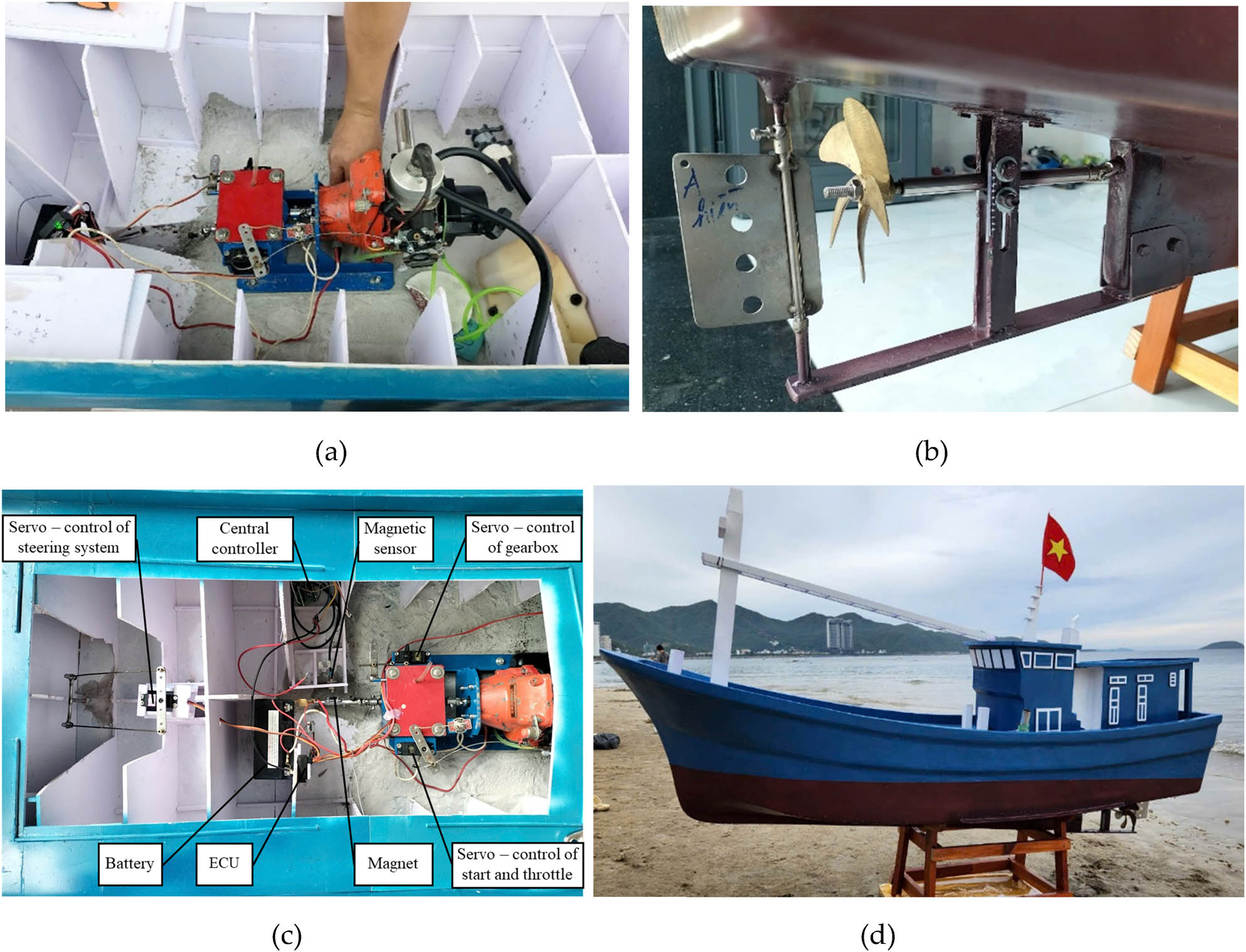
Details of fabrication of the model hull: (a) engine room layout; (b) adjustable propeller shaft inclination mechanism; (c) arrangement of the control system; and (d) completed model vessel.
For a control system, the scaled model control system allows for precise operation during tests while ensuring data acquisition. It had a remote control unit that could start, stop, throttle, shift gears, and steer the rudder, all within 200 m. Integrated sensors enabled real-time monitoring of the propeller shaft speed through Bluetooth, sending data to a mobile device up to 70 m away, as illustrated in Figure 8c. Accurate speed calculations were possible through laser-based distance measurement (within ±1.5 mm margin of error; maximum margin of error distance 100 m), coupled with high-precision stopwatches (with 1/1,000th of a second accuracy). The subsystem underwent extensive evaluations for stability and integration with propulsion and steering systems, providing a stable base for investigational studies regarding shaft inclination.
This fully assembled model replicated closely with the actual ship form and function, including essential systems such as the propulsion system (∼4.4 kW total input power), adjustable shaft distance component, and control components. It also made changing the variable being tested easy and facilitated multiple experiments. The final model was performed stably and reliably during all design and testing periods. Such a detailed fabrication process established that the scaled model accurately reflected the actual vessel, a prerequisite for reliable experimental and numerical studies (shown in Figure 8d).
2.3 Experimental setup
The study was carried out on a model scaled from an actual ship in a towing tank, where the propeller shaft was inclined at different angles to determine how inclination affects ship performance. For verification, the model draft was corrected to achieve hydrodynamic similarity with the fully loaded draft of the actual ship. Inclination angles of the propeller shaft from 0° to 15° were tested in 1° increments, while the propeller shaft rotational speed was constant for all tests. This technique reduced variation (caused by voltage changes) and provided regularity. Unlike in open waters, the towing tank allowed for calm water conditions, with a vastly subdued environment resulting in better data quality. The model’s speed was recorded over an established 50 m test distance with a high-accuracy laser distance meter (accuracy of ±1.5 mm) and a stopwatch with a resolution of 1/1,000th of a second. The velocity was calculated from the measured distance divided by the recorded time, equivalent to the model’s speed for the corresponding shaft inclination angle.
The experimental setup utilized Bluetooth-activated sensors to record and transmit real-time data from the propeller shaft on a mobile device. This meant that all tests were conducted consistently. The model was controlled from the rear and would keep straight, maintaining a straight line while minimizing errors due to instability or lateral drift. Each inclination angle was performed three times to enable repeatability, and the average velocity was used for evaluation. In addition, it was shown that the resistance values derived using the Holtrop method were well consistent with the measurements derived experimentally and using numerical predictions. The sizeable experimental setup produced repeatable and reliable results, lending itself to forming a solid model for determining vessel speed about the incline of the propeller shaft and validating the results of numerical models.
These processes were carefully developed to ensure the accuracy and reliability of the experiment. The draft of the scaled model was set to the fully loaded draft of the actual vessel, preserving geometric and hydrodynamic similarity. Specifically, the initial trials were carried out with an incline angle of 3° for the propeller shaft, which matched the arrangement of the actual vessel. To eliminate power fluctuations affecting the results, the speed of the propeller shaft was accurately tracked and maintained constant for all inclination angles. The distance of the testing was chosen so that there would be stable motion at a constant propeller speed, keeping the total error less than 5%. This was possible by running at full throttle under maximum speed, which reached a velocity of 3.77 knots (1.94 m/s), and by allowing an error of ±0.5 m (distance) and ±1.0 s (time). All the above experimental procedures were operated as a schematic diagram of Figure 9.
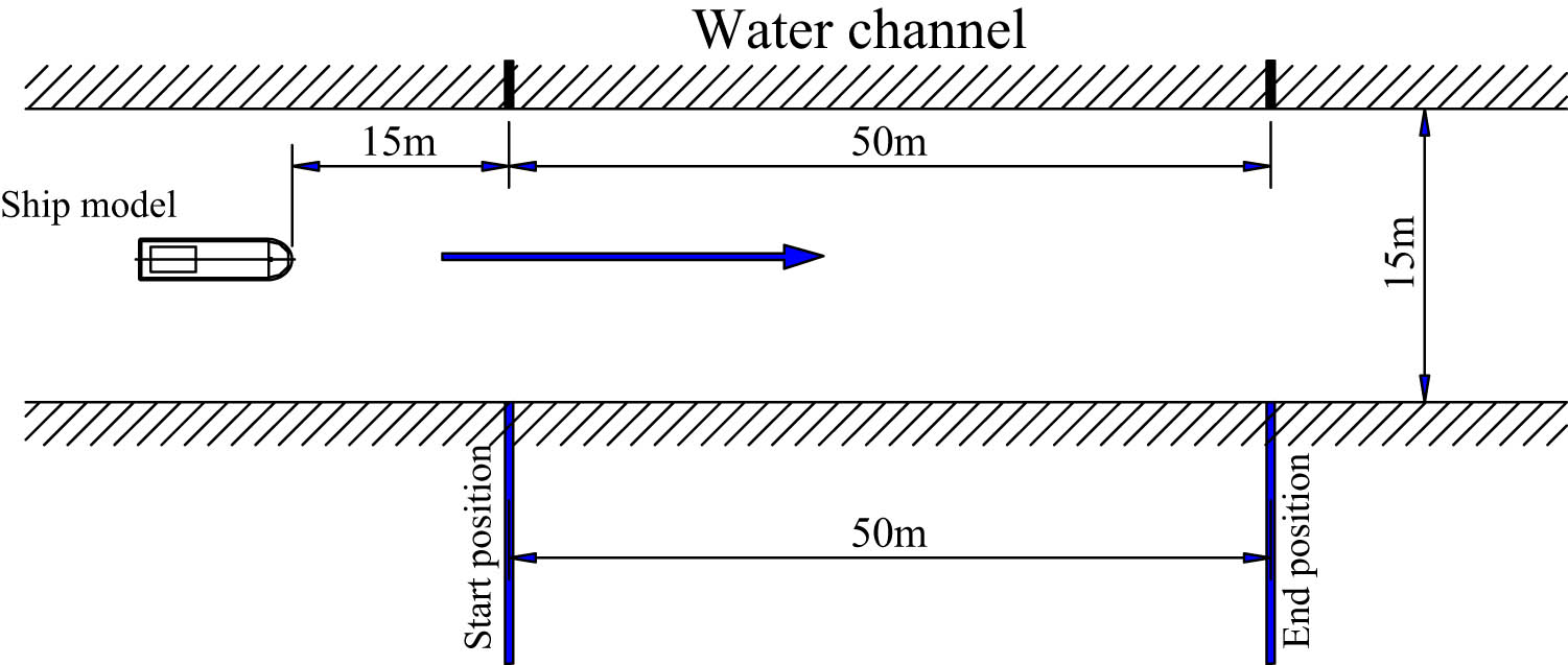
Schematic diagram for the experiment.
2.4 Numerical simulations
Recently, the nonlinear finite-element method has been one of the ideal ways to evaluate ship structures for ocean engineering [22,23,24,25,26]. Numerical simulations evaluated the hydrodynamic performances of the scaled model and the full-scale vessel at different propeller shaft inclination angles. CFD tools were used to simulate the approximate parameters [27]. These simulations confirmed the results obtained by experiments and provided a complete picture of the vessel’s response.
The computational domain was configured to reflect the towing tank environment, with sufficiently sized boundaries to minimize interference effects. The domain utilized a structured hexahedral mesh, ensuring high-quality elements for numerical solutions. The computational domain was discretized into a structured mesh of 9.2 million elements and a hull surface of 1.5 million faces. Element sizings were optimized to capture essential flow features: the most diminutive element dimensions at the hull were 0.0007 m, and the largest, located far from the hull, was 0.02 m; high-resolution meshing at the bow and stern regions ensured that flow separation and wake details were accurately modeled, as shown in Figure 10.
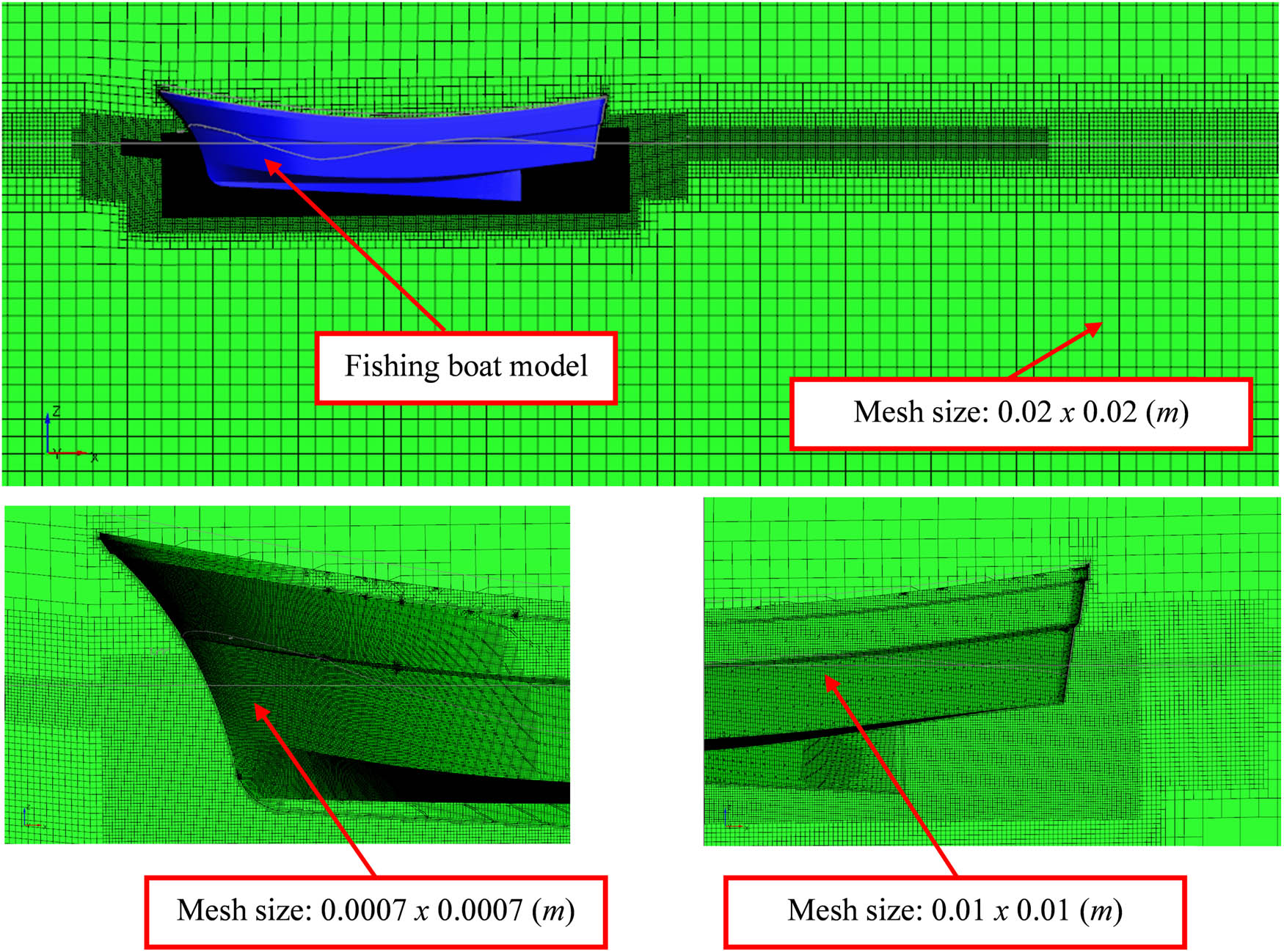
Numerical simulation setups.
Boundary conditions were implemented to emulate the physical conditions experienced in towing tank experiments. The 3D model was developed in ANSYS FLUENT, where a uniform velocity profile was established at the inlet boundary, and the outlet boundary was defined as a “pressure outlet” to allow free outflow from the system. The hull surface was set as a no-slip wall as it is directly interacting with the water, and the boundaries were set as slip walls to avoid reflection effects during the far fields. The RANS approach was used to solve the governing equations using the turbulence model, which is known to provide a good compromise between computational speed and accuracy, to properly resolve the turbulent and near-wall flow field.
3 Experimental and numerical results
After the scale model was fabricated (as outlined in Section 2.2), this section reports the speed measurements obtained for varying propeller shaft angles up to 15° applied under three operating conditions, namely design speed of 2.9 knots and supplementary speeds of 2.31 and 3.46 knots. CFD results for the same inclination angles are also compared with the experiments.
3.1 Experimental results
3.1.1 Experimental testing at the design speed of 2.9 knots
The experimental tests performed at the design speed of 2.9 knots aim to assess the vessel’s operational efficiency at various angles of inclination of the propeller shaft. The main goal is to know how the shaft inclination affects the vessel’s speed, verifying if the experimental results can be similar to theoretical predictions and numerical simulations. Table 4 shows the experimental error between the theoretical and measured results for the testing procedure and error analysis, whereby the tests were conducted over a 50 m length course chosen to ensure stability and minimize experimental error. The total error was constrained to be less than 5% for the chosen distance (0.5 m for distance and 1.0 s for time). Such conditions enabled accurate measurements, especially when stability becomes paramount at the design speed when the average velocity is applied to reduce random errors.
Error analysis for distance and time measurements during testing
| Distance (m) | Time (s) | Distance error (%) | Time error (%) | Total error (%) |
|---|---|---|---|---|
| 10 | 5.15 | 5.00 | 19.40 | 24.40 |
| 15 | 7.73 | 3.33 | 12.93 | 16.27 |
| 20 | 10.31 | 2.50 | 9.70 | 12.20 |
| 25 | 12.89 | 2.00 | 7.76 | 9.76 |
| 30 | 15.46 | 1.67 | 6.47 | 8.13 |
| 35 | 18.04 | 1.43 | 5.54 | 6.97 |
| 40 | 20.62 | 1.25 | 4.85 | 6.10 |
| 45 | 23.20 | 1.11 | 4.31 | 5.42 |
| 50 | 25.77 | 1.00 | 3.88 | 4.88 |
| 55 | 28.35 | 0.91 | 3.53 | 4.44 |
| 60 | 30.93 | 0.83 | 3.23 | 4.07 |
Table 5 shows the measurements of the velocities at various inclination angles, and these results are depicted in Figure 11. For the setting with a 3° inclination angle, which corresponds to the actual configuration of the vessel, the measured velocity was 2.9 knots, equal to the design speed. At inclination angles from 0° and 3°, the increased speed was also very high, at 0° 2.47 knots, while at 3° it has the design speed (an increase of 14.8%). In practical terms, this means the changes made to the propeller shaft’s angle for optimal charging significantly impact vessel speed due to reduced resistance. At 3° and 8°, the velocity was less than their peak, with peaks recorded at 6° and 7° recording 3.05 knots or 5.2% above the design speed. These outcomes suggest the presence of an optimum range of shaft angles in which the thrust direction is well suited to fit the hull geometry to reduce resistance at a specific speed range. After 8°, speed started easing off dramatically, dropping from 2.98 knots at 8° to 1.92 knots at 15° (32.6% decrease). At a neglecting shaft tilt angle, the hydrodynamic equilibrium was maintained, such that the force volume was used fully, which caused a peak thrust; when the inclination was increased, this peak decreased considerably, which means the thrust system was disturbed, and high friction occurred.
Measured time and calculated velocity of the model vessel at a design speed of 2.9 knots
| Propeller shaft inclination angle (°) | Time (s) | Speed | Propeller shaft inclination angle (°) | Time (s) | Speed | ||
|---|---|---|---|---|---|---|---|
| m/s | knot | m/s | knot | ||||
| 0 | 39.29 | 1.27 | 2.47 | 8 | 32.57 | 1.53 | 2.98 |
| 1 | 37.40 | 1.34 | 2.60 | 9 | 34.04 | 1.47 | 2.85 |
| 2 | 35.22 | 1.42 | 2.76 | 10 | 35.03 | 1.43 | 2.77 |
| 3 | 33.47 | 1.49 | 2.90 | 11 | 36.92 | 1.35 | 2.63 |
| 4 | 32.68 | 1.53 | 2.97 | 12 | 38.52 | 1.30 | 2.52 |
| 5 | 32.15 | 1.56 | 3.02 | 13 | 42.11 | 1.19 | 2.31 |
| 6 | 31.80 | 1.57 | 3.05 | 14 | 45.93 | 1.09 | 2.11 |
| 7 | 31.86 | 1.57 | 3.05 | 15 | 50.46 | 0.99 | 1.92 |
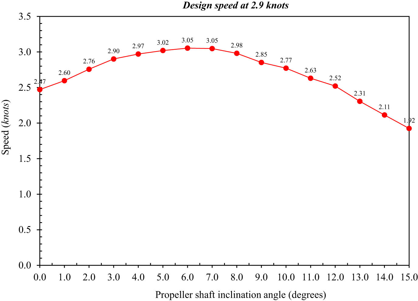
Variation of vessel speed with propeller shaft inclination angle at a design speed of 2.9 knots.
The velocity trends illustrated in Figure 11 suggest that, for maximum velocity, the optimal shaft inclination will be slightly above the design configuration, approximately between 6.0° and 7.0°. Coupled with the relatively stable performance maintained in this band suggests that the thrust produced by the propeller is more closely aligned with the hull, limiting losses of energy. However, suppose the orientation is sampled toward the extremes at both ends (below 3.0° and above 8.0°). In that case, it leads to poor performance, stressing the importance of accurately adjusting the shaft inclination.
3.1.2 Experimental testing at the design speed of 2.31 knots and 3.46 knots
Two more tests were performed to understand the effect of the interaction between propeller shaft inclination angle and another parameter influencing vessel speed, at speeds of 2.31 knots and 3.46 knots corresponding to the full-scale vessel speeds of 8.0 knots and 12.0 knots. The tests were intended to confirm that speed variation for each type was consistent across different operating conditions. The same experimental setup and methodology were used for a design speed of 2.9 knots. Tables 6 (2.31 knots) and 7 (3.46 knots) show the results of the two additional cases. The top tables show time measurements, and the bottom displays the calculated velocities.
Measured time and calculated velocity of the model vessel at a speed of 2.31 knots
| Propeller shaft inclination angle (°) | Time (s) | Speed | Propeller shaft inclination angle (°) | Time (s) | Speed | ||
|---|---|---|---|---|---|---|---|
| m/s | knot | m/s | knot | ||||
| 0 | 49.35 | 1.01 | 1.97 | 8 | 40.44 | 1.24 | 2.40 |
| 1 | 46.98 | 1.06 | 2.07 | 9 | 41.46 | 1.21 | 2.34 |
| 2 | 44.29 | 1.13 | 2.19 | 10 | 43.37 | 1.15 | 2.24 |
| 3 | 42.01 | 1.19 | 2.31 | 11 | 46.41 | 1.08 | 2.09 |
| 4 | 41.02 | 1.22 | 2.37 | 12 | 48.59 | 1.03 | 2.00 |
| 5 | 40.41 | 1.24 | 2.40 | 13 | 52.75 | 0.95 | 1.84 |
| 6 | 40.03 | 1.25 | 2.43 | 14 | 57.56 | 0.87 | 1.69 |
| 7 | 40.00 | 1.25 | 2.43 | 15 | 63.37 | 0.79 | 1.53 |
At the 2.31 knots speed showed a similar trend as the design speed case in Figure 12. Within the range of 0°–3.0°, a rapid increase in speed was noted, whereas the receiver’s highest speed of 2.43 knots was found at inclination angles of 6.0° and 7.0° with an increase rate of 5.2% compared to at 3.0°. The speed dropped significantly after 7.0°, reaching 1.53 knots at 15°, a decrease of 33.7%. These results show that at lower speeds, the optimum shaft inclination angles are the same as the design speed case, confirming the importance of aligning shaft and hull geometry. The patterns of variation in speed, especially at the design and lower speed levels, provided some quite interesting differences for the higher speed of 3.46 knots, with the figures (Figure 12) quite illuminating. A maximum speed of 3.53 knots also occurred at a 5.0° angle of inclination, which is below the desired value range obtained in other cases. Beyond 5°, the speed started to drop more dramatically with the increase in the inclination angle, down to 1.25 knots at 15.0°, a decrease of 64.6% from the horizontal case. This variation indicates that at high speeds, the interaction between the propeller thrust and hull hydrodynamics becomes more sensitive to the variation in inclination output.
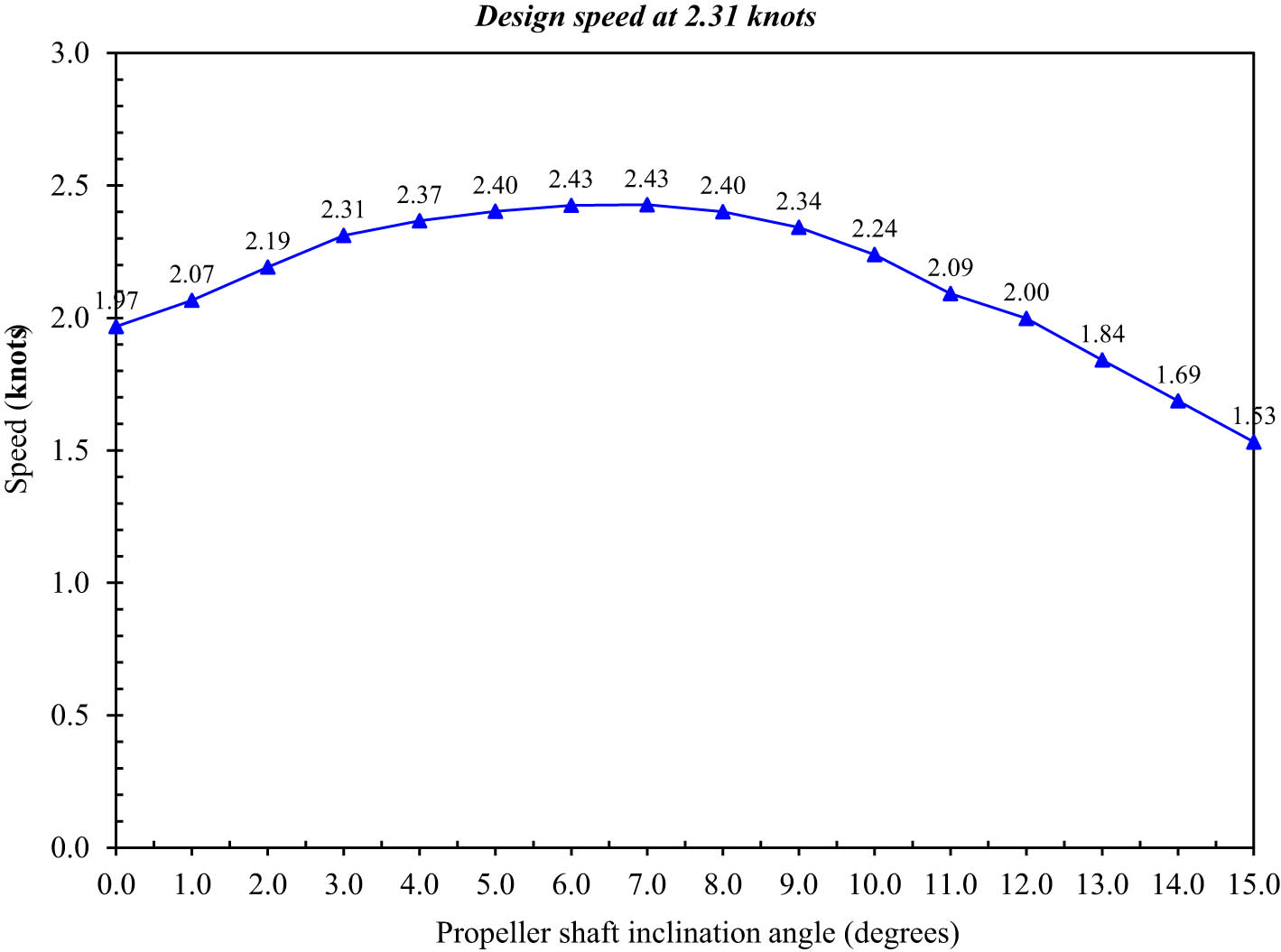
Variation of vessel speed with propeller shaft inclination angle at a speed of 2.31 knots.
Figure 13 displays a comparative approach regarding how speed varies among the three test cases, revealing steady patterns for design and lower speeds, with the best inclination angles lying between 6.0° and 7.0°. If we check the figure at a higher speed around 3.46 knots, the ideal angle changes to 5.0° (Figure 13). At elevated speeds, dynamic pressure and wave formation are more pronounced, and more control has to be exercised for the optimal propeller shaft angle (Table 7).
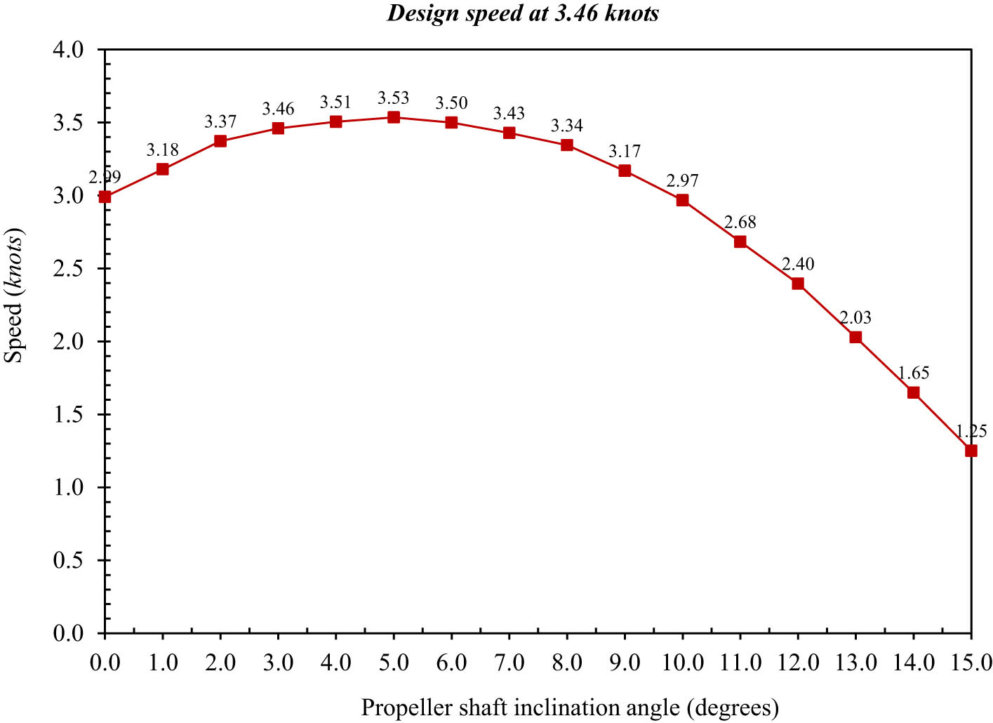
Variation of vessel speed with propeller shaft inclination angle at a speed of 3.46 knots.
Measured time and calculated velocity of the model vessel at a speed of 3.46 knots
| Propeller shaft inclination angle (°) | Time (s) | Speed | Propeller shaft inclination angle (°) | Time (s) | Speed | ||
|---|---|---|---|---|---|---|---|
| m/s | knot | m/s | knot | ||||
| 0 | 32.47 | 1.54 | 2.99 | 8 | 29.03 | 1.72 | 3.34 |
| 1 | 30.54 | 1.64 | 3.18 | 9 | 30.64 | 1.63 | 3.17 |
| 2 | 28.79 | 1.74 | 3.37 | 10 | 32.72 | 1.53 | 2.97 |
| 3 | 28.06 | 1.78 | 3.46 | 11 | 36.20 | 1.38 | 2.68 |
| 4 | 27.70 | 1.81 | 3.51 | 12 | 40.53 | 1.23 | 2.40 |
| 5 | 27.47 | 1.82 | 3.53 | 13 | 47.87 | 1.04 | 2.03 |
| 6 | 27.75 | 1.80 | 3.50 | 14 | 58.88 | 0.85 | 1.65 |
| 7 | 28.32 | 1.77 | 3.43 | 15 | 77.66 | 0.64 | 1.25 |
3.2 Numerical results
The CFD simulations were performed to analyze the vessel’s hydrodynamic characteristics at various propeller shaft angle inclinations, supplementing the experimental data. Whenever the vessel was 0° to 15° inclined, the numerical model was performed for a design speed of 2.9 knots. The results can be observed in Table 8 and can be visualized in Figures 13–16. Table 8 shows the CFD simulation results for different inclination angles based on the velocity of the vessels, which can also be seen in Figure 13. The velocity trends are in good agreement with the experimental results, confirming the validity of the numerical method. The simulated speed at 3.0° was 2.93 knots, coinciding with the design speed value with a difference of less than 1% from the experimental one. The velocity increased steadily up to 6.0° and 7.0°, where the highest simulated velocity (3.07 knots) was registered, corresponding to a 5.9% increase compared to the speed at 3.0°. Above 7.0°, the speed dropped rapidly, and at 15°, it fell to 2.06 knots, 32.8% less than the maximum.
Simulated velocity results for the model vessel at a speed of 2.9 knots
| Propeller shaft inclination angle (°) | Velocity (knots) | Propeller shaft inclination angle (°) | Velocity (knots) |
|---|---|---|---|
| 0 | 2.53 | 8 | 3.03 |
| 1 | 2.66 | 9 | 2.95 |
| 2 | 2.8 | 10 | 2.84 |
| 3 | 2.93 | 11 | 2.71 |
| 4 | 3.00 | 12 | 2.58 |
| 5 | 3.05 | 13 | 2.41 |
| 6 | 3.07 | 14 | 2.25 |
| 7 | 3.07 | 15 | 2.06 |
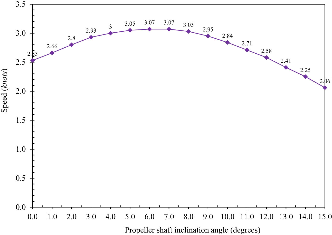
Variation of vessel speed with propeller shaft inclination angle at the design speed of 2.9 knots.
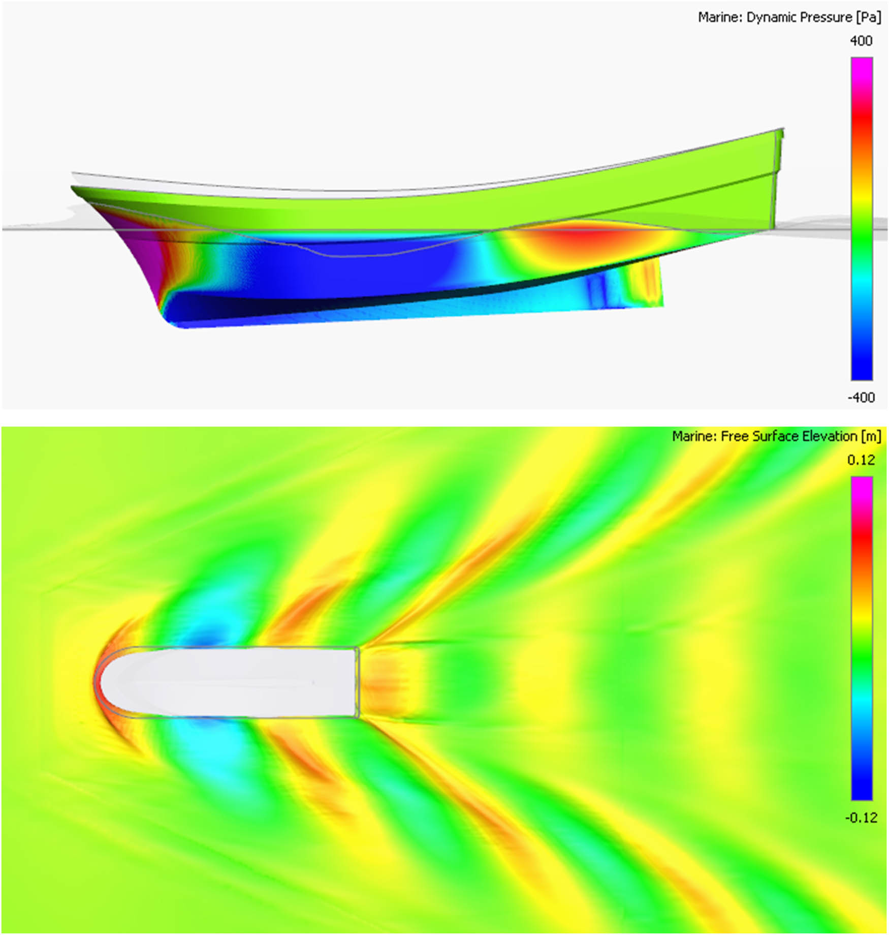
Pressure distribution and wave patterns around the hull at a propeller shaft inclination angle of 0°.
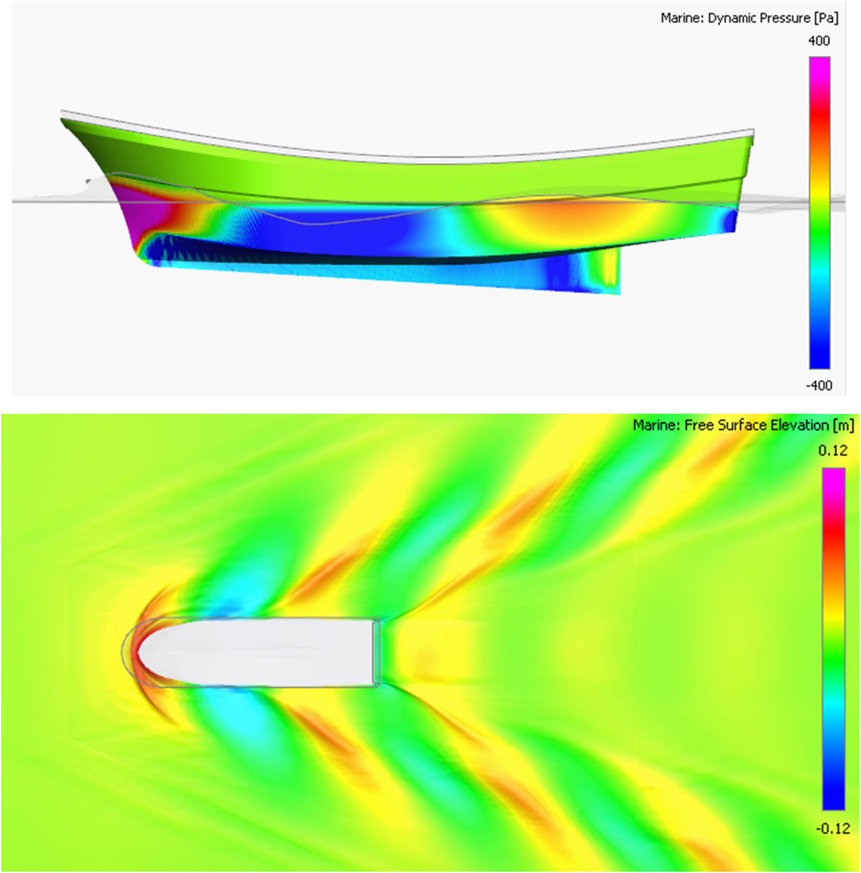
Pressure distribution and wave patterns around the hull at propeller shaft inclination angles of 6° and 7°.
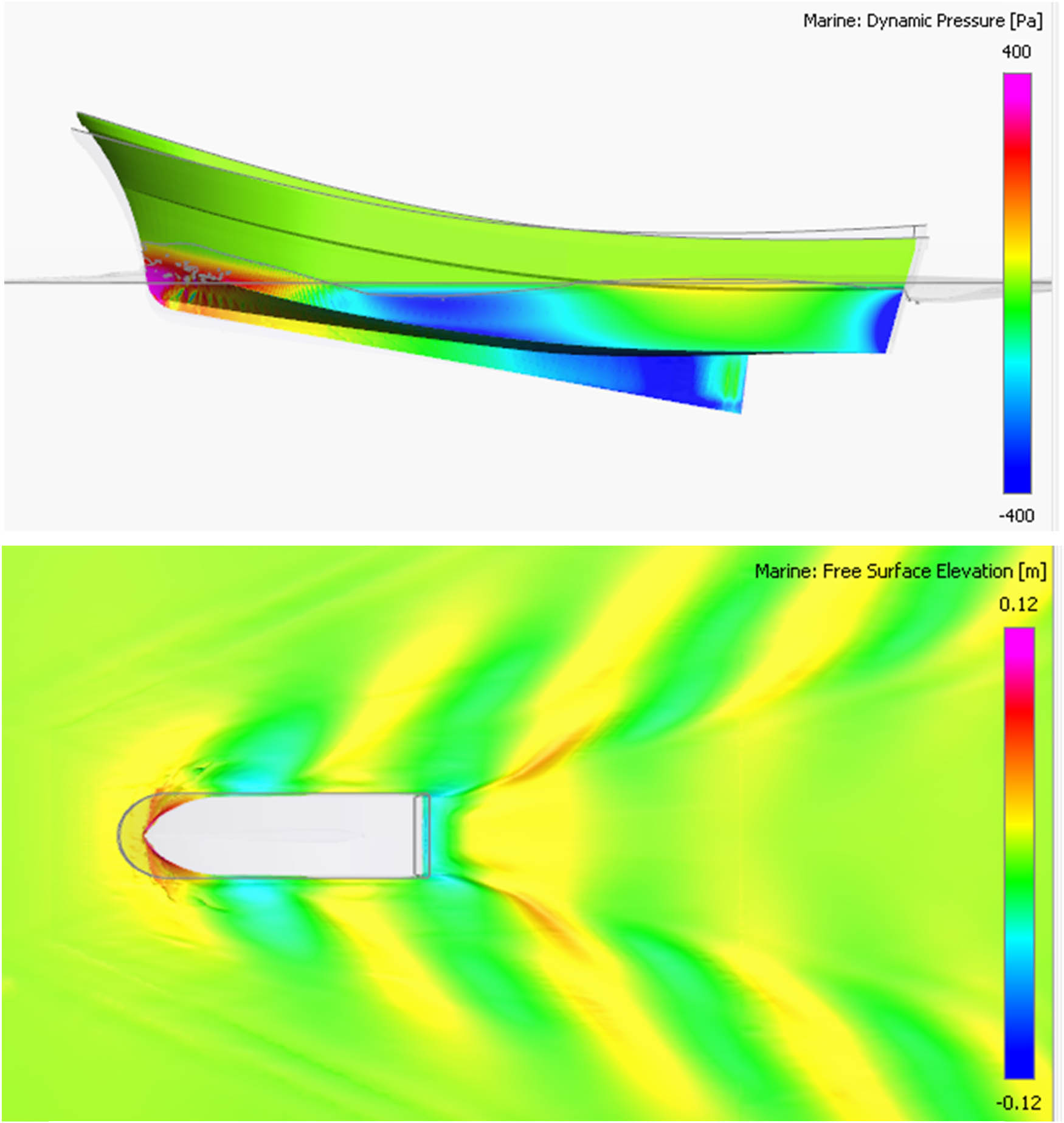
The CFD simulations were analyzed for the flow characteristics and the pressure distributions around the hull at different inclination angles. The wave field and pressure fields of the thrust force acting at 0° averaged over 90 points are shown in Figure 15 (where the thrust force and resistance coincide). This means higher resistance and a speed of 2.53 knots. As shown in Figure 16, at the optimal inclination angles of 6° and 7°, the thrust force will be aligned efficiently with the hull geometry, thus reducing resistance. This reduces the bow pressure and minimizes the wave energy around the hull. Again, this contributes to achieving the maximum speed of 3.07 knots. However, at 15°, based on Figure 17, the excessive inclination leads to the thrust force and the hydrodynamic flow not overlapping. As a result, the bow presses bigger waves, causing a loss of energy and a drastic reduction in vessel speed.
Pressure distribution and wave patterns around the hull at a propeller shaft inclination angle of 15°.
4 Discussion
After the scale model was fabricated (as outlined in Section 2.2), this section reports the speed measurements obtained for varying propeller shaft angles up to 15° applied under three operating conditions, namely design speed of 2.9 knots and supplementary speeds of 2.31 and 3.46 knots. Also, the CFD simulation results at the design speed of the same range of inclination angles are given and compared with the experimental data.
4.1 Fabricated model composite fishing vessel and test results
A 1:12 scale model of the composite fishing vessel was carefully fabricated to accurately show the same size, shape, and characteristics as the actual ship. Formex sheets and fiberglass composite ensured structural solidity with low weight, and the deck and cabin were separately manufactured for manufacturing agility and maintenance services. Equipped with a 0.8 HP gasoline engine that serves as the main propulsion and an adjustable propeller shaft mechanism, the inclination was accurately adjustable between 0° and 15° to ensure reliable experimental outputs. The Bluetooth-based remote-control system with enabling sensors worked well up to 200 m, allowing for real-time monitoring and continuous data collection.
The model exhibited stability in light and heavily loaded modes with a top speed of 3.77 knots, swimming 30 percent faster than the design speed. Although small amendments, like errors in surface finishing, exist, the model could describe the hydrodynamic performance of the real ship. It was designed and fitted in such a way that it became a robust tool for experimental and numerical studies to testify to the study’s findings. Improvements can be made in the long term with tighter surface finishing and new materials for increased accuracy.
The findings contribute to a deeper understanding of how different propeller shaft angles can be tuned for optimal vessel performance, presenting essential trends and ideal setups. It is noted that tests were performed under controlled conditions to facilitate repeatability, consistency, and accuracy of the data recording. These results closely match the theoretical predictions and have real-world implications for vessel design and operation.
Indeed, as the propeller shaft inclination angle increased from 0° to 3.0°, the experimental data showed that the vessel speed increased from 2.47 knots at 0° to 2.9 knots at 3.0°, meaning an improvement of 14.8%. This indicates that, with a low angle of inclination, the direction of the thrust is more in line with the geometry of the hull itself, reducing resistance and promoting propulsion. At 3.0°–8.0°, the speed gradually plateaued; the peak speed was recorded at 6.0° and 7.0°, 3.05 knots or 5.2% above the design speed, as illustrated in Figure 19. The shaft angles in this range produce the optimal shaft angle for the scaled model when the resultant hydrodynamic forces acting on the propeller jet are most favorably aligned. In values 8° and higher, speed sharply drops to 1.92 knots at 15° with a 32.6% decline from the peak. The assertion is that too much inclination leads to a counter-productivity when propulsion can no longer be matched to the hydrodynamics of the hull, producing increased resistance and loss of efficiency.
The change in vessel speed was found in the tilt angle of the propeller shaft from 0° to 15°, as shown in Figure 16. At 2.31 knots, the speed variation pattern appears very similar to that at 2.9 knots, aside from the slight differences recorded at minor inclination angles (0°–1.0°) and significant angles (13°–15°). This consistency indeed reflects the similar hydrodynamic behavior for these two speeds. The 3.46 knots speed variation, on the other hand, describes a noticeably different pattern. Notably, the rate of change appears to decrease in the 8.0° < γ < 9.0° range to help max out the speed achieved at a 5° inclination angle, where the ship achieves a max speed of 3.53 knots compared with the lower speed ranged found at the 6°–7° angle. At higher angles of attack (beyond 5.0°), the speed drops significantly, especially the decline between 6.0° and 15.0° becomes steeper, revealing that as we increase operating speed, we also increase the influence of resistance due to flow separation and wake turbulence (Figure 18).
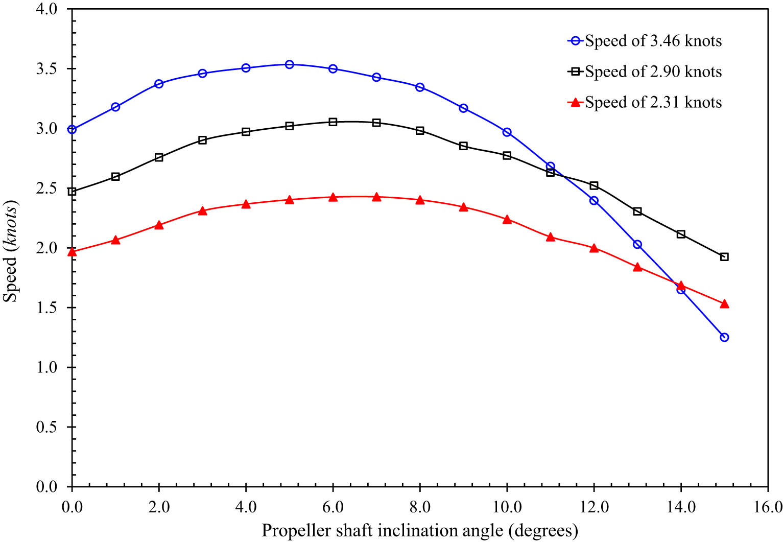
Variation of vessel speed with a propeller shaft inclination angle for each speed.
Table 9 analyzes speed deviations at different inclination angles relative to the baseline angle 3°. In the example with the second most minor deviation (2.31 knots), the distance was only 0.78 knots at 15°, then the distance was found to bow at 0.98 knots in the 2.9 knot case, and 3.46 knots had the most significant deviation of 2.21 at 15°. These results suggest that speed mismatches are more critical when the entire speed range is more extensive. This behavior illustrates the strong influence of propeller shaft angle on the vessel’s operation, especially for more comprehensive and higher-speed shapes, as hydrodynamic forces and flow dynamics become more responsive to small changes in inclination.
Speed deviations at various propeller shaft inclination angles compared to the baseline (3°)
| Propeller shaft inclination angle (°) | Case of speed 2.31 knots | Case of speed 2.9 knots | Case of speed 3.46 knots | ||||||
|---|---|---|---|---|---|---|---|---|---|
| Speed (knots) | Speed deviation (knots) | Sai số (%) | Speed (knots) | Speed deviation (knots) | Sai số (%) | Speed (knots) | Speed deviation (knots) | Sai số (%) | |
| 0 | 1.97 | −0.34 | −14.83 | 2.47 | −0.43 | −14.80 | 2.99 | −0.47 | −13.58 |
| 1 | 2.07 | −0.24 | −10.54 | 2.60 | −0.30 | −10.49 | 3.18 | −0.28 | −8.13 |
| 2 | 2.19 | −0.12 | −5.11 | 2.76 | −0.14 | −4.94 | 3.37 | −0.09 | −2.54 |
| 3 | 2.31 | 0.00 | 0.00 | 2.90 | 0.00 | 0.00 | 3.46 | 0.00 | 0.00 |
| 4 | 2.37 | 0.06 | 2.45 | 2.97 | 0.07 | 2.43 | 3.51 | 0.05 | 1.31 |
| 5 | 2.40 | 0.09 | 4.01 | 3.02 | 0.12 | 4.13 | 3.53 | 0.07 | 2.15 |
| 6 | 2.43 | 0.12 | 4.98 | 3.05 | 0.15 | 5.28 | 3.50 | 0.04 | 1.12 |
| 7 | 2.43 | 0.12 | 5.07 | 3.05 | 0.15 | 5.07 | 3.43 | −0.03 | −0.93 |
| 8 | 2.40 | 0.09 | 3.94 | 2.98 | 0.08 | 2.78 | 3.34 | −0.12 | −3.35 |
| 9 | 2.34 | 0.03 | 1.38 | 2.85 | −0.05 | −1.65 | 3.17 | −0.29 | −8.41 |
| 10 | 2.24 | −0.07 | −3.09 | 2.77 | −0.13 | −4.42 | 2.97 | −0.49 | −14.24 |
| 11 | 2.09 | −0.22 | −9.44 | 2.63 | −0.27 | −9.31 | 2.68 | −0.78 | −22.48 |
| 12 | 2.00 | −0.31 | −13.50 | 2.52 | −0.38 | −13.09 | 2.40 | −1.06 | −30.77 |
| 13 | 1.84 | −0.47 | −20.32 | 2.31 | −0.59 | −20.50 | 2.03 | −1.43 | −41.38 |
| 14 | 1.69 | −0.62 | −26.98 | 2.11 | −0.79 | −27.11 | 1.65 | −1.81 | −52.34 |
| 15 | 1.53 | −0.78 | −33.67 | 1.92 | −0.98 | −33.65 | 1.25 | −2.21 | −63.87 |
The stable trends observed for 2.31 and 2.9 knots indicate that the ideal inclination angle is between 6.0° and 7.0° for those ships operating at moderate speeds. On the contrary, at faster speeds, where we can talk about a speed of 3.46 knots, the best inclination changes to 5.0°, given that, with the same impeller, there is greater sensitivity on the flow dynamics/resistance at higher speeds. At higher velocities from the shaft angle, there is a rapid drop-off in speed past 5.0°, reinforcing that accurate shaft alignment is required to maintain energy losses further. It is suggested that vessels operating at moderate speeds should retain the shaft propeller at an inclination angle of 6.0°–7.0°, and for higher-speed vessels, an inclination angle of about 5°. In all situations, ensure that extreme inclination angles (13.0°–15.0°) are avoided, as they cause colossal speed loss and inefficiencies.
4.2 Comparison of CFD simulation and model vessel test results
A comparison between CFD simulations and experimental results for the scaled model can be used to evaluate the accuracy and reliability of the numerical approach. Both Table 10 and Figure 19 present the analysis, emphasizing the primary similarities and differences between the conventional and proposed methods for diverse propeller shaft inclination angles, illustrating the comparative advantages and disadvantages of the two methods. Table 10 demonstrates that the simulated and experimental velocities align well for most inclination angle values, especially in the optimal range of 3°–7°. The average difference between the simulated and experimental results is about 1.0%, indicating that the CFD model sufficiently captured the hydrodynamic behavior of the scaled vessel. However, as the inclination angle decreases from 8° to 15°, the error shows a rising trend. At inclination angles of 14° and 15°, the error exceeds 5%. Overall, the velocity discrepancies between the simulation and experimental results are negligible, confirming that the simulation model demonstrates acceptable reliability.
Comparison of CFD simulation and experimental results for the model vessel at a speed of 2.9 knots
| Propeller shaft inclination angle (°) | Speed (knots) | Error (%) | |
|---|---|---|---|
| Test | Numerical simulation | ||
| 0 | 2.47 | 2.53 | 2.34 |
| 1 | 2.60 | 2.66 | 2.42 |
| 2 | 2.76 | 2.80 | 1.55 |
| 3 | 2.90 | 2.93 | 1.00 |
| 4 | 2.97 | 3.00 | 0.98 |
| 5 | 3.02 | 3.05 | 0.99 |
| 6 | 3.05 | 3.07 | 0.55 |
| 7 | 3.05 | 3.07 | 0.75 |
| 8 | 2.98 | 3.03 | 1.63 |
| 9 | 2.85 | 2.95 | 3.32 |
| 10 | 2.77 | 2.84 | 2.40 |
| 11 | 2.63 | 2.71 | 2.96 |
| 12 | 2.52 | 2.58 | 2.31 |
| 13 | 2.31 | 2.41 | 4.34 |
| 14 | 2.11 | 2.25 | 6.05 |
| 15 | 1.92 | 2.06 | 6.59 |
| Mean | 2.51 | ||
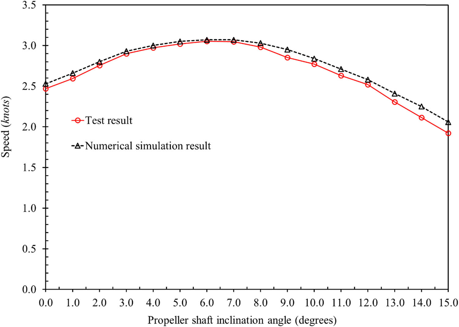
Comparison of vessel speed variation with changes in a propeller shaft inclination angle.
Examining the flow characteristics shown in Figures 14–16, the results are as follows: At angles of inclination of 6.0° and 7.0° (where the highest speeds are obtained), the thrust direction is more optimal with the hull shape and velocity. This causes the vessel’s bow to lift slightly, resulting in lower pressure distribution at the bow. Simultaneously, the wave energy is reduced around the hull (Figure 15). This results in a fluid approach with a lower pressure distribution and wave energy, resulting in lower total force acting against the vessel, enabling the ship to operate at higher velocities.
In any pitch angle of inclination at 0°, as seen in Figure 14, the thrust direction matches the same direction of the resistance force. As a result, there is virtually no change in the bow and stern drafts during operation. Here, at this angle, the bow draft is also greater than in 6.0° and 7.0° cases, which causes higher pressure at the bow area. Furthermore, higher total resistance and slower speeds of the vessel than the most optimal inclination range were detected because the wave energy produced surrounding the hull surface was higher.
At a 15.0° angle of inclination (Figure 16), we observe that the excessive thrust angle concerning the draft raises the bow too much and lowers the stern. Indeed, this development leads to orders of magnitude greater pressure distribution at the bow value than for the 6.0° and 7.0° cases. On the contrary, the energy of the wave generated for the hull surface is approaching that of the 0° incidence angle. As a result, the total resistance increases, and the vessel operates at lower speeds than in the other cases.
This study shows that the inclination of the propeller shaft is instrumental in managing those factors to achieve an optimal thrust alignment and internal pressure distribution for the wave energy encounter that determines a vessel’s resistance and speed. These insights will help ensure that this simulation not only accurately replicates real-world dynamics but also that shaft inclination is optimized for performance.
4.3 Numerical simulation for an actual composite fishing boat
Given the high reliability of the simulated velocities for the scaled model, CFD software was further utilized in this study to simulate the speed of the full-scale vessel for propeller shaft inclination angles ranging from 3° to 8°. The simulation results and comparisons to actual vessel speeds are presented in Table 11. At the actual propeller shaft inclination angle of 3°, the discrepancy between simulated and real-world speeds was negligible at 2.2%, indicating a strong correlation between the simulation and actual performance. The highest simulated speed for the full-scale vessel was achieved at a 6° inclination angle, reaching 11.45 knots, representing a 14.5% increase compared to the actual speed at 3°.
Comparison of simulated and actual speeds for the full-scale vessel
| Propeller shaft inclination angle (°) | Actual speed (knots) | Numerical speed (knots) | Error (%) |
|---|---|---|---|
| 3 | 10.00 | 10.22 | 2.20 |
| 4 | — | 10.59 | 5.90 |
| 5 | — | 10.97 | 9.70 |
| 6 | — | 11.45 | 14.50 |
| 7 | — | 11.37 | 13.70 |
| 8 | — | 10.96 | 9.60 |
| Mean | 9.27 | ||
Installing a propeller shaft at the optimal inclination angle (in this case, 6°) significantly enhances vessel speed, contributing to improved economic efficiency during operations – precisely, increased vessel speed without altering the engine’s operational regime results in reduced fuel consumption. Moreover, higher vessel speeds shorten travel time at sea, saving time and enhancing the quality of caught products by decreasing the preservation duration onboard. These findings underscore the critical importance of optimizing propeller shaft inclination for maximizing vessel performance and operational efficiency. These findings are consistent with previous studies by Santoso et al. [1], which proved that the optimal angle of the propeller shaft inclination is between 6° and 7° for moderate speeds. The trend found in the high-speed case (optimal near 5°) is in agreement with Seyyedi et al. [8].
5 Conclusion
Based on experimental results, this study developed and simulated a scaled composite fishing vessel model that produced significant results regarding the propeller shaft inclination angles and vessel speed performance. The confirmed numerical simulations of the experimental data showed that the ideal inclination angle of the vessel’s propeller shaft varied from 6.0° to 7.0°, providing a maximum speed of 3.05 knots, 5.2% above the design speed. These discoveries highlight the importance of orienting the thrust direction per the hull shape to reduce resistance and enhance efficiency.
In addition, the study presented that due to the increase in resistance and hydrodynamic of vessels, the extensive inclination angles (>8.0°) cause a considerable slowdown of the boats. Conversely, the optimal angle varies at higher operational speeds, highlighting the dynamic interplay between operating speed, hydrodynamic forces exerted on the shaft, and shaft alignment.
The results also emphasize the potential operational gains from targeting propeller shaft inclination angles in full-scale vessels. Continuous improvements in ship speed at the same engine regime result in less fuel consumption, shorter voyages, and better product quality due to fewer cargo preservation times on the sea. These enhancements increase the economic efficiency of fishing operations.
Future work would be to study the effect of varying immersion depths concerning inclination angles, as this variable impacts the hydrodynamic forces received by the propeller blades. Moreover, introducing new computation techniques and diversifying resistance calculation methods will further optimize the precision of power and performance calculation methods. This would help in a few areas that would improve the knowledge and use of hydrodynamic optimization in the design of fishing vessels. This study sets a robust finding for practical applications, and guides improved composite fishing vessel performance, providing meaningful progress in naval architecture and ocean engineering.
Acknowledgments
The authors would like to thank Nha Trang University for supporting the experimental facilities and computational resources used in this study.
-
Funding information: The authors would like to thank Nha Trang University for supporting this research under grant number TR2023-13-38.
-
Author contributions: All authors have accepted responsibility for the entire content of this manuscript and approved its submission.
-
Conflict of interest: The authors state no conflict of interest.
-
Data availability statement: The data supporting the findings of this study are available from the corresponding author upon reasonable request.
References
[1] Santoso A, Arief IS, Masro’i N, Semin S. Effect of main engine placement and propeller shaft inclination on ship performance. Int J Mar Eng Innov Res. 2021;6(1):53–64.10.12962/j25481479.v6i1.6510Search in Google Scholar
[2] Van NT. Dynamics study of the motion of forest fire extinguishing boats. Doctoral thesis. Hanoi, Vietnam: Vietnam National University of Forestry; 2017.Search in Google Scholar
[3] Savitsky D. Hydrodynamic design of planing hulls. Mar Technol. 1964;1(1):71–95.10.5957/mt1.1964.1.4.71Search in Google Scholar
[4] Bate J. Performance analysis and prediction of high-speed planing craft. Doctor Philosophia. Plymouth, United Kingdom: University of Plymouth;1994.Search in Google Scholar
[5] Skupień E, Prokopowicz J. Methods of calculating ship resistance on limited waterways. Pol Marit Res. 2015;21(4):12–7.10.2478/pomr-2014-0036Search in Google Scholar
[6] DOOSAN Infracore. Installation instructions. Incheon, South Korea; 2020.Search in Google Scholar
[7] Hien NV. Application of CFD theory to calculate resistance of high-speed composite hull ships. Master’s thesis. Nha Trang, Vietnam: Nha Trang University; 2020.Search in Google Scholar
[8] Seyyedi SM, Shafaghat R, Siavoshian M. Experimental study of immersion ratio and shaft inclination angle in the performance of a surface-piercing propeller. Mech Sci. 2019;10:153–67.10.5194/ms-10-153-2019Search in Google Scholar
[9] Cong-Nghi T. Ship design handbook. Ho Chi Minh, Vietnam: Construction Publishing House; 2008.Search in Google Scholar
[10] Birk L. Fundamentals of ship hydrodynamics: Fluid mechanics, ship resistance and propulsion. USA: John Wiley & Sons Ltd; 2019.10.1002/9781119191575Search in Google Scholar
[11] Duc-An N, Ban N. Ship theory – Volume 2. Ho chi Minh, Vietnam: Transport Publishing House; 2006.Search in Google Scholar
[12] Ngoc-Tu T, Thanh-Hai PT, Manh-Chien N. Study on the effect of model scale on the change in flow characteristics surrounding the hull using the CFD method. Sci Technol J. 2023;3:2023.Search in Google Scholar
[13] Hetharia WR, de Fretes ER, Gaspersz F. Computational and experimental works on ship resistance. Int Conf Mar Sci Technol. 2019;339:012036.10.1088/1755-1315/339/1/012036Search in Google Scholar
[14] Zhang C, Ringsberg JW, Thies F. Development of a ship performance model for power estimation of inland waterway vessels. Ocean Eng. 2023;287:115731.10.1016/j.oceaneng.2023.115731Search in Google Scholar
[15] Thi-Ha-Phuong N, Thi-Hai-Ha N. Prediction of resistance for KVLCC2 model ship using STAR-CCM + software. Sci Technol J – Univ Danang. 2020;18(9):7–10.Search in Google Scholar
[16] Le HTH, Dinh-Tu T. Simulation study of fluid flow through fishing vessel hulls considering the influence of propellers and rudders. Sci Technol J – Fish. 2024;2:2024.Search in Google Scholar
[17] Holtrop J. A statistical re-analysis of resistance and propulsion data. ISP. 1984;31(363):272–6.Search in Google Scholar
[18] Holtrop J, Mennen GGJ. An approximate power prediction method. Int Shipbuild Prog. 1982;29(335):166–70.10.3233/ISP-1982-2933501Search in Google Scholar
[19] Van Oortmerssen G. A power prediction method and its application to small ships. Int Shipbuild Prog. 1971;18(207):397–415.10.3233/ISP-1971-1820701Search in Google Scholar
[20] Pham T, Le QT, Do QT. Experimental and numerical investigations of multi-layered ship engine room bulkhead insulation thermal performance under fire conditions. Curved Layer Struct. 2024;11:20240006.10.1515/cls-2024-0006Search in Google Scholar
[21] Nhut P, Tien DD, Do QT. Evaluating deformation in FRP boat: Effects of manufacturing parameters and working conditions. J Mech Behav Mater. 2024;33:20220311.10.1515/jmbm-2022-0311Search in Google Scholar
[22] Do QT, Ghanbari-Ghazijahani T, Prabowo AR. Developing empirical formulations to predict residual strength and damages in tension-leg platform hulls after a collision. Ocean Eng. 2023;286:115668.10.1016/j.oceaneng.2023.115668Search in Google Scholar
[23] Do QT, Van Huynh V, Vu MT, Van Tuyen V, Pham-Thanh N, Tra TH, et al. A new formulation for predicting the collision damage of steel stiffened cylinders subjected to dynamic lateral mass impact. Appl Sci. 2020;10:1–30.10.3390/app10113856Search in Google Scholar
[24] Do QT, Huynh VV, Cho SR, Vu MT, Vu QV, Thai DK. Residual ultimate strength formulations of locally damaged steel stiffened cylinders under combined loads. Ocean Eng. 2021;225:108802.10.1016/j.oceaneng.2021.108802Search in Google Scholar
[25] Fath A, Kusuma F, Muttaqie T, Prabowo AR, Sukanto H, Tampubolon BD, et al. Investigating the influence of plate geometry and detonation variations on structural responses under explosion loading: A nonlinear finite-element analysis with sensitivity analysis. Curved Layer Struct. 2024;11:20240019.10.1515/cls-2024-0019Search in Google Scholar
[26] Maulana F, Prabowo AR, Ridwan R, Ubaidillah U, Ariawan D, Sohn JM, et al. Antiballistic material, testing, and procedures of curved-layered objects: A systematic review and current milestone. Curved Layer Struct. 2023;10:20220200.10.1515/cls-2022-0200Search in Google Scholar
[27] Tran TG, Nguyen HV, Van Huynh Q. A method for optimizing the hull form of fishing vessels. J Ship Res. 2023;67:72–91.10.5957/JOSR.05210017Search in Google Scholar
© 2025 the author(s), published by De Gruyter
This work is licensed under the Creative Commons Attribution 4.0 International License.
Articles in the same Issue
- Research Articles
- Layerwise generalized formulation solved via a boundary discontinuous method for multilayered structures. Part 1: Plates
- Thermoelastic interactions in functionally graded materials without energy dissipation
- Layerwise generalized formulation solved via boundary discontinuous method for multilayered structures. Part 2: Shells
- Visual scripting approach for structural safety assessment of masonry walls
- Nonlinear analysis of generalized thermoelastic interaction in unbounded thermoelastic media
- Study of heat transfer through functionally graded material fins using analytical and numerical investigations
- Analysis of magneto-aerothermal load effects on variable nonlocal dynamics of functionally graded nanobeams using Bernstein polynomials
- Effective thickness of gallium arsenide on the transverse electric and transverse magnetic modes
- Investigating the behavior of above-ground concrete tanks under the blast load regarding the fluid-structure interaction
- Numerical study on the effect of V-notch on the penetration of grounding incidents in stiffened plates
- Thermo-elastic analysis of curved beam made of functionally graded material with variable parameters
- Effect of curved geometrical aspects of Savonius rotor on turbine performance using factorial design analysis
- A mechanical and microstructural investigation of friction stir processed AZ31B Mg alloy-SiC composites
- Mechanical design of engineered-curved patrol boat hull based on the geometric parameters and hydrodynamic criteria
- Review Article
- Technological developments of amphibious aircraft designs: Research milestone and current achievement
- Special Issue: TS-IMSM 2024
- Influence of propeller shaft angles on the speed performance of composite fishing boats
- Design optimization of Bakelite support for LNG ISO tank 40 ft using finite element analysis