Dynamic of a nonautonomous two-species impulsive competitive system with infinite delays
-
Mengxin He


Abstract
In this paper, we consider a nonautonomous two-species impulsive competitive system with infinite delays. By the impulsive comparison theorem and some mathematical analysis, we investigate the permanence, extinction and global attractivity of the system, as well as the influence of impulse perturbation on the dynamic behaviors of this system. For the logistic type impulsive equation with infinite delay, our results improve those of Xuxin Yang, Weibing Wang and Jianhua Shen [Permanence of a logistic type impulsive equation with infinite delay, Applied Mathematics Letters, 24(2011), 420-427]. For the corresponding nonautonomous two-species impulsive competitive system without delays, we discuss its permanence, extinction and global attractivity, which weaken and complement the results of Zhijun Liu and Qinglong Wang [An almost periodic competitive system subject to impulsive perturbations, Applied Mathematics and Computation, 231(2014), 377-385].
1 Introduction
The logistic system is considered to be one of the most important systems in mathematical ecology, and a great deal of research works have been done based on this system. Because of the seasonal fluctuations in the environment and hereditary factors, many scholars have investigated the logistic system with time delays (see [1, 2, 3, 4, 5, 6, 7, 8]). Noticing that the disturbance of environmental factors at certain time moments can give rise to instantaneous and changes of population density, many scholars have investigated the dynamic behaviors of impulsive differential equations (see [9, 10, 11, 12, 13, 14, 15, 16, 17, 18, 19, 20, 21]). Especially, Yang [21] investigated the following logistic system with infinite delay
with the initial condition x(t) = ϕ(t), t ≤ 0, which is continuous and bounded on (−∞, 0] to [0, +∞) with ϕ(0) > 0. Here a(t) and b(t) are continuous functions, bounded above and below by positive constants; K : [0, +∞) → (0, +∞) is a continuous kernel such that
which implies hk ≤ 1 is an increase sequence.
On the other hand, competition for limited resources among ecologically similar species has been intensively investigated by many scholars due to its extensive prevalence and its importance on determining the structure of animal and plant communities, the diversity and the evolution of species. The famous Lotka-Volterra competition system has been studied extensively (see [22, 23, 24]). Naturally, impulse perturbations have been introduced into competitive systems and many excellent results have been obtained (see [13, 18, 25, 26, 27, 28, 29, 30, 31, 32]). Recently, Liu and Wang [32] considered an almost periodic impulsive competitive system of the form
For any given continuous function f(t), let fL and fM denote inf0≤t<+∞ f(t) and sup0≤t<+∞ f(t), respectively. The authors discussed the permanence of system (1.2) under the following conditions:
Π0<tk<t hik, i = 1, 2, are bounded above and below by positive constants for all t > 0;
riL − biM > 0, i = 1, 2.
But the authors did not consider its competition exclusion, global attractivity and extinction. For the permanence of system (1.2), we also want to know whether conditions (H1) and (H2) can be weakened? To answer this question, we first introduce the following example.
Example 1.1
For system (1.2), let
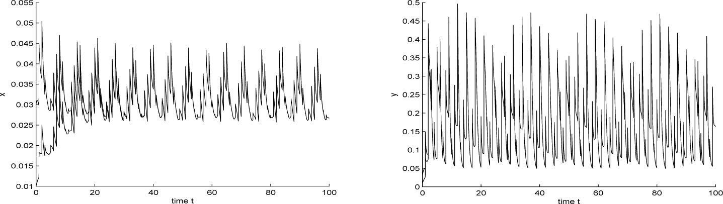
System (1.2) with the initial conditions (0.01, 0.01)T and (0.03, 0.03)Trespectively
This example gives a certain answer to the above question. So it requires us to give its strict mathematical verification and to discuss the competition exclusion, global attractivity and extinction of (1.2). Our results improve and complement the corresponding results of Liu and Wang [32].
Motivated by the above papers, in this paper we consider the following system
under an initial condition
Here x1(t) and x2(t) are population densities of species x1 and x2 at time t respectively; r1(t) > 0 and r2(t) > 0 are the growth rates; a1(t) > 0 and a2(t) > 0 are the effects of intra-specific competition; ri(t) and ai(t) are continuous functions, bounded above and below by positive constants for all t > 0; the continuous functions b1(t) ≥ 0 and b2(t) ≥ 0 are the rates of inter-specific competition, which are bounded for all t > 0; Ki : [0, +∞) → (0, +∞) (i = 1, 2) are continuous kernels such that
2 Preliminaries
In this section, we present the following definitions and lemmas which are useful in proving our main results.
Let PC([0, +∞), R2) = {ϕ : [0, +∞) → R+ × R+, ϕ is continuous for t ≠ tk. Also
Define Gk = (tk−1, tk) × R+ × R+, k = 1, 2, …; G =
Definition 2.1
Let V ∈ V0. For any (t, X(t)) ∈ [tk−1, tk) × R+ × R+, the right-hand derivative D+ V(t, X(t)) along the solution X(t, X0) of system (1.3) is defined by
Lemma 2.1
(see [10]) Assume that m ∈ PC[R+, R] with points of discontinuity at t = tk is left continuous at t = tk, k = 1, 2, …, and that
where g ∈ C[R+ × R+, R], ϕk ∈ C[R, R] and ϕk(u) is nondecreasing in u for each k = 1, 2, …. Let r(t) be the maximal solution of the scalar impulsive differential equation
existing on [t0, +∞), then
Remark 2.1
(see [10]) In Lemma 2.1, assume inequalities (2.1) reverse. Let p(t) be the minimal solution of (2.1) existing on [t0, +∞), then
Consider the following impulsive system
where a and b are positive constants.
Lemma 2.2
(see [17]), Let y(t) be any positive solution of system (2.3). It follows that:
If hL ≥ 1, then
If hL < 1, hM < 1 and aθ + ln hL > 0, then
If hL < 1, hM ≥ 1 and aθ + ln hL > 0, then
Lemma 2.3
Let y(t) be any positive solution of system (2.3). Assume that aη + ln hM ≤ 0. Then
Proof
Let z(t) = 1/y(t), then system (2.3) is transformed into
According to [9], for any T > 0, we can obtain
First we consider aη + ln hM = 0, that is
Next consider aη + ln hM < 0, that is
because of
Lemma 2.4
Let (x1(t), x2(t))T be any solution of system (1.3) with (1.4), then xi(t) > 0, i = 1, 2, for all t ≥ 0.
Proof
From the ith equation of (1.3) with (1.4) (i = 1, 2), we can obtain
where 1 ≤ j ≤ 2, i ≠ j, which completes the proof of Lemma 2.4.
Lemma 2.5
For any y ∈ PC([0, +∞), R+), let k : [0, +∞) → (0, +∞) be a continuous kernel such that
The proof is similar to that of Lemma 3 in [24], so we omit it.
3 Main results
In this section, we present the main results of this paper. First we study the coexistence of system (1.3).
Theorem 3.1
Let (x1(t), x2(t))T be any solution of system (1.3) with (1.4), i = 1, 2. Assume that
then
with
Proof
From (1.3), we can obtain for i = 1, 2 that
Then according to Lemma 2.1, we have
For i = 1, 2, substituting this into the ith equation of (1.3), we obtain
If hiM ≥ 1, it follows that
where
If hiM < 1, we have
where
All the above analysis show that
Therefore for any given ε > 0 satisfying
there exists a T > 0 such that for t > T, xi(t) ≤ Mi + ε, i = 1, 2.
Substituting this into system (1.3), it follows from Lemma 2.5 that, for 1 ≤ i, j ≤ 2 and i ≠ j
We can easily obtain that
Substituting this into the ith equation of system (1.3) gives rise to
Next we prove
If hiL ≥ 1, we deduce that
By setting ε → 0, it follows from Lemma 2.2 that
where
If hiL < 1, we obtain
By setting ε → 0, it follows from Lemma 2.2 that
where
Thus,
This proves the permanence of (1.3).
Theorem 3.2
Suppose that the conditions of Theorem 3.1 holds, and there exist σi > 0 and ρi > 0 such that
and
where Mi and mi (i = 1, 2) are defined in Theorem 3.1. Then for any two solutions (x1(t), x2(t))T and (y1(t), y2(t))T of system (1.3) with (1.4), there are
Proof
Let (x1(t), x2(t))T and (y1(t), y2(t))T be any two solutions of system (1.3) with (1.4). From Theorem 3.1, for any ε1 > 0 satisfying 0 < ε1 < min{m1, m2}, there exist δ > 0 such that
and T1 > 0 such that for t > T1,
Define a Lyapunov function as follows
For t > T1 and t ≠ tk, k = 1, 2, …, calculating the upper right derivatives of V1i(t) with 1 ≤ i, j ≤ 2 and i ≠ j, we have
where ξj(t) lies between xj(t) and yj(t), j = 1, 2.
For i = 1, 2, define
For t > T1 and t ≠ tk, k = 1, 2, …, calculating the upper right derivatives of V2i(t), it follows that
Denote Vi(t) = V1i(t) + V2i(t) for i = 1, 2. Therefore, for t > T1 and t ≠ tk, k = 1, 2, …,
where ξij(t) (1 ≤ i, j ≤ 2; i ≠ j) lies between xi(t) and yi(t), i = 1, 2.
For t = tk, we can easily verify that
Therefore, V(t) is bounded on [T1, +∞) and there is
Similarly to the analysis of [17], it is obvious that
This completes the proof of Theorem 3.2.
Next, we consider the competition exclusion of system (1.3).
Theorem 3.3
Let (x1(t), x2(t))T be any solution of system (1.3) with (1.4). Assume that
then the species x1 is permanent but the species x2 is extinct, that is
where M1 is defined in Theorem 3.1 and
with
Proof
Since (3.9) implies that r1M θ + ln h1L > 0, according to the proof of Theorem 3.1 there is
According to Lemmas 2.1 and 2.3, we have
Then for any ε2 > 0 satisfying
Substituting this into system (1.3), it follows from Lemma 2.5 that
Similarly we have
Then similarly to the analysis of Lemma 2.2, by setting ε2 → 0 we can easily obtain
with
This completes the proof of the theorem.
Consider the following impulsive system
Theorem 3.4
Under the assumptions of Theorem 3.3, we further suppose that there exists a σ1 > 0 such that
Then for any positive solution (x1(t), x2(t))T of system (1.3), and any positive solution x(t) of system (3.12), there is
Proof
Let (x1(t), x2(t))T be any positive solution of system (1.3), and x(t) be any positive solution of system (3.12). From the condition of Theorem 3.6, there exists a δ1 > 0 such that
According to Theorem 3.5, for any 0 < ε3 < m̄1 small enough, there exists a T3 > 0 such that for t > T3,
Define a Lyapunov function as follows
Similarly to the analysis of Theorem 3.2, for t > T3 and t ≠ tk, k = 1, 2, …, calculating the upper right derivatives of V̄1(t), we can obtain
Define
For t > T3 and t ≠ tk, k = 1, 2, …, calculating the upper right derivatives of V̄2(t) and denoting V̄(t) = V̄1(t) + V̄2(t), it follows that
By the boundedness of x1(t) and x(t) and setting ε3 → 0, we educe that
For t = tk, we can easily verify that
Therefore, V̄(t) is bounded on [T3, +∞) and there is
Similarly to the analysis of [17], it is obvious that
This completes the proof of Theorem 3.4.
Now we discuss the extinction of system (1.3).
Theorem 3.5
Let (x1(t), x2(t))T be any positive solution of system (1.3). Assume that
then system (1.3) is extinct, that is
Proof
The proof of the theorem is similar to the corresponding part of Theorem 3.3, so we omit the detail.
In the following part of this section, based on the above theorems, we gives some corresponding results for systems (1.1) and (1.2) respectively. First for system (1.1), similarly to the analysis of Theorems 3.1 and 3.2, we can easy obtain the following theorem.
Theorem 3.6
Let x(t) and y(t) be any two positive solutions of system (1.1). Assume that
Then system (1.1) is permanent and globally attractive, that is
where
with
Remark 3.1
In Corollary 3.1, we prove the global attractivity of (1.1), but under some weaker conditions than those in Yang [21]; especially, our result does not require the following unreasonable condition:
Next for system (1.2), similarly to the proof of Theorem 3.1, we can easily prove the following theorem.
Theorem 3.7
Let (x1(t), x2(t))T be any solution of system (1.2) with xi(0) > 0, i = 1, 2. Assume that
then
Theorem 3.8
Under the conditions of Theorem 3.7, we further assume that there exist ρ1 > 0 and ρ2 > 0 such that
Then for any two positive solutions (x1(t), x2(t))T and (y1(t), y2(t))T of system (1.2), there are
Proof
Let (x1(t), x2(t))T and (y1(t), y2(t))T be any two positive solutions of system (1.2). From Theorem 3.7, for any ε4 > 0 small enough, there exist δ2 > 0 satisfying
Define a Lyapunov function as follows
For t > T4 and t ≠ tk, k = 1, 2, …, calculating the upper right derivatives of Ṽ(t), for j = 1, 2 and j ≠ i, we have
where ζj(t) lies between xj(t) and yj(t).
For t = tk, we can easily verify that
Therefore, Ṽ(t) is bounded on [T4, +∞) and there is
Similarly to the analysis of [17], it is obvious that
This completes the proof of Theorem 3.8.
Consider the following impulsive system
Similarly to the analysis of Theorems 3.7 and 3.8, we can easily prove the following theorem.
Theorem 3.9
Let (x1(t), x2(t))T be any positive solution of system (1.2), x(t) be any positive solution of system (3.14). Assume that
Then the species x1 is permanent and globally attractive but the species x2 is extinct, that is
where
Theorem 3.10
Let (x1(t), x2(t))T be any solution of system (1.2) with xi(0) > 0, i = 1, 2. Assume that
then system (1.2) is extinct, that is
Proof
By impulsive comparison theorem and Lemma 2.3, these results can be easily obtained, so we omit the detail.
Remark 3.2
Obviously, condition (H1) implies (3.13), but not vice versa. Thus Theorem 3.7 weakens Lemma 2.4 in [32]. Also Theorems 3.8-3.10 complement the results of [32].
4 Numerical simulation
In this section, we present some numerical simulations to show the influence of impulse perturbations on the dynamic behaviors of systems.
In Table 1, by calculation we have r1L = 0.8, r1M = 0.88, a1L = 0.27, a1M = 0.29, b1L = 0.01, b1M = 0.012, h1L = 0.9, h1M = 1.3, r2L = 0.3, r2M = 0.36, a2L = 0.1, a2M = 0.12, b2L = 0.02, b2M = 0.022, h2L = 1.01, h2M = 1.09, θ = 0.5, η = 1. Choose ρ1 = 9 and ρ2 = 5. Therefore,
Parameter values of system (1.3)
| Parameter | Interpretation | Value |
|---|---|---|
| r1(t) | Growth rate of species x1 | |
| r2(t) | Growth rate of species x2 | |
| a1(t) | Intra-specific competition of species x1 | 0.28+0.01sin |
| a2(t) | Intra-specific competition of species x2 | 0.11 + 0.01 sin 2t |
| b1(t) | Interspecific competition o of species x2 on x1 | 0.011 + 0.001 sin t |
| b2(t) | Interspecific competition o of species x1 on x2 | 0.021 + 0.001 sin t |
| K1(t) | Kernel function of species x1 | 10e−10t |
| K2(t) | Kernel function of species x2 | 8e−8t |
| h1k | Impulse perturbations on species x1 | 1.1 − 0.2 cos k |
| h2k | Impulse perturbations on species x2 | 1.05 + 0.04 sin 2k |
| tk | Impulse points | k + |
We can easily verify that
Thus all the conditions of Theorem 3.2 are satisfied. Therefore both species x1 and x2 are permanent and globally attractive, which is shown in Figure 2.
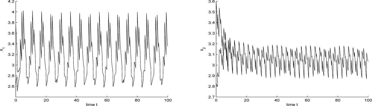
System (1.3) with (ϕ1(t), ϕ2(t)) = (2.6, 2.8)T and (3.8, 3.6)T for t ≤ 0 respectively.
Furthermore, we keep the growth rates, the intra-specific competition and the kernel functions of all species unchanged in Table 1, but adjust the values of the impulse perturbations given in Table 2, then simulations (see Figures 3-5) show that the permanence and extinction of the species are significantly changed, which are in accordance with the results of Theorems 3.4 and 3.5, here we can verify the corresponding conditions similarly to those in Table 1.
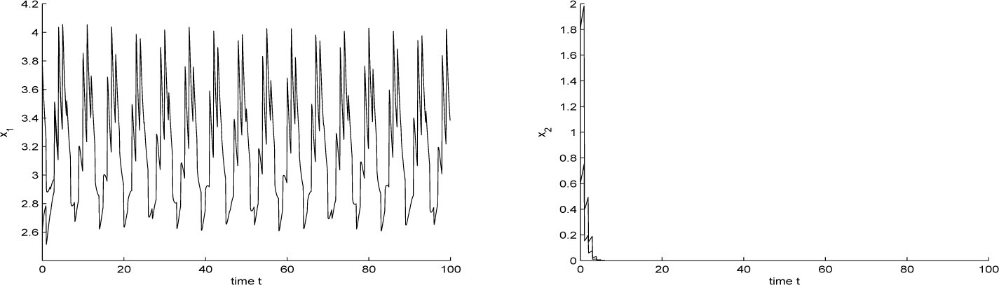
System (1.3) with (ϕ1(t), ϕ2(t)) = (3.8, 0.6)T and (2.6, 1.8)T for t ≤ 0 respectively.
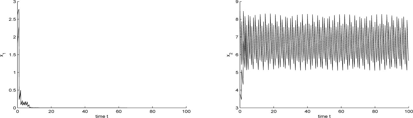
System (1.3) with (ϕ1(t), ϕ2(t)) = (2.6, 3.8)T and (1.8, 8.6)T for t ≤ 0 respectively.
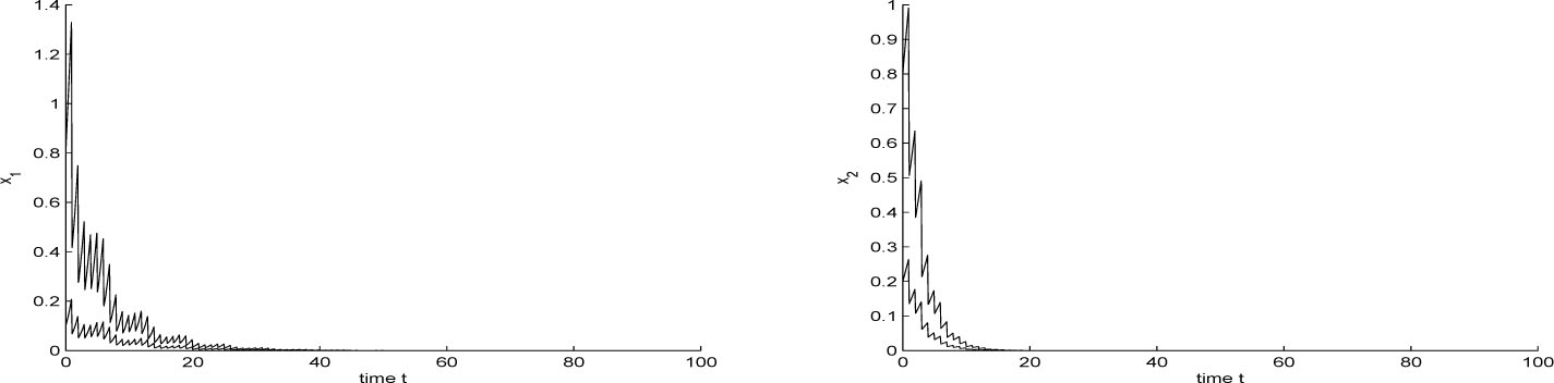
System (1.3) with (ϕ1(t), ϕ2(t)) = (0.1, 0.8)T and (0.8, 0.2)T for t ≤ 0 respectively.
5 Conclusion
In this paper, we are devoted to obtaining the major factors that affect the coexistence, competition exclusion and extinction of system (1.3). Table 1 shows that we can choose some suitable values of parameters of system (1.3) to guarantee the coexistence of both species. However, when we change the values of the impulse perturbations shown in Table 2, there is a significant variation of the survival of each species. When choo sing the impulse perturbations hik < 1 small enough and keeping the value of the growth rate unchanged, it is hard to maintain the permanence of the species xi. Moreover, this can result in the extinction of both species, which is different from the continuous system. The impulse perturbation plays an important role in the survival of the species and can deduce more situations of real ecosystems. Furthermore, for the logistic type impulsive equation with infinite delay, our results improve those of [21] and remove its unreasonable condition. For the corresponding nonautonomous two-species impulsive competitive system without delays, our results weaken and complement the results of [32].
Acknowledgements
The research was supported by the Scientic Research Foundation of Fuzhou University under Grant GXRC-18062.
References
[1] Wright E.M., A non-linear differential equation, J. Reine Angew. Math., 1955, 194, 66-8710.1515/crll.1955.194.66Search in Google Scholar
[2] Kuang Y., Delay Differential Equations: with Applications in Population Dynamics, 1993, Boston: Academic Press.Search in Google Scholar
[3] Seifert G., Almost periodic solutions for delay Logistic equations with almost periodic time dependence, Differ. Integral Equ., 1996, 9, 335-34210.57262/die/1367603350Search in Google Scholar
[4] Feng C.H., On the existence and uniqueness of almost periodic solutions for delay Logistic equations, Appl. Math. Comput., 2003, 136, 487-49410.1016/S0096-3003(02)00072-3Search in Google Scholar
[5] Chen F.D., Shi C.L., Dynamic behavior of a Logistic type equation with infinite delay, Acta Math. Appl. Sinica, 2006, 22, 313-32410.1007/s10255-006-0307-6Search in Google Scholar
[6] Yang X.T., The existence and asymptotic behavior of almost periodic solution for the Logistic equations with infinite delay, J. Systems Sci. Math. Sci., 2001, 21, 405-408Search in Google Scholar
[7] Teng Z.D., Permanence and stability in non-autonomous Logistic systems with infinite delays, Dyn. Stab. Syst., 2002, 17, 187-20210.1080/14689360110102312Search in Google Scholar
[8] Li H.X., Almost periodic solutions for logistic equations with infinite delay, Appl. Math. Lett., 2008, 21, 113-11810.1016/j.aml.2007.02.013Search in Google Scholar
[9] Bainov D.D., Simeonov P.S., Impulsive Differential Equations: Periodic Solutions and Applications, 1993, New York; Longman Scientificand Technical.Search in Google Scholar
[10] Lakshmikantham V., Bainov D.D., Simeonov P.S., Theory of impulsive differential equations, 1989, World Scientific.10.1142/0906Search in Google Scholar
[11] Saker S.H., Oscillation and global attractivity of impulsive periodic delay respiratory dynamics model, Chin. Ann. Math. Ser., 2005, B26, 511-52210.1142/S0252959905000403Search in Google Scholar
[12] Stamov G.T., On the existence of almost periodic solutions for the impulsive Lasota-Wazewska model, Appl. Math. Lett., 2009, 22, 516-52010.1016/j.aml.2008.07.002Search in Google Scholar
[13] He M.X., Chen F.D., Li Z., Almost periodic solution of an impulsive differential equation model of plankton allelopathy, Nonlinear Anal. RWA, 2010, 11, 2296-230110.1016/j.nonrwa.2009.07.004Search in Google Scholar
[14] Liu X.N., Chen L.S., Global dynamics of the periodic logistic system with periodic impulsive perturbations, J. Math. Anal. Appl., 2004, 289, 279-29110.1016/j.jmaa.2003.09.058Search in Google Scholar
[15] Yan X.H., Almost Periodic solution of the Logistic equation with impulses, J. Hefei Univ., 2013, 3, 7-10Search in Google Scholar
[16] Sun S.L., Chen L.S., Existence of positive periodic solution of an impulsive delay Logistic model, Appl. Math. Comput., 2007, 184, 617-62310.1016/j.amc.2006.06.060Search in Google Scholar
[17] He M.X., Chen F.D., Li Z., Permanence and global attractivity of an impulsive delay Logistic model, Appl. Math. Lett., 2016, 62, 92-10010.1016/j.aml.2016.07.009Search in Google Scholar
[18] He M.X., Li Z., Chen F.D., Dynamics of an impulsive model of plankon allelopathy with delays, J. Appl. Math. Comput., 2017, 55, 749-76210.1007/s12190-016-1069-9Search in Google Scholar
[19] Xie Y.X., Wang L.J., Deng Q.C., Wu Z.J., The dynamics of an impulsive predator Cprey model with communicable disease in the prey species only, Appl. Math. Comput., 2017, 292, 320-33510.1016/j.amc.2016.07.042Search in Google Scholar
[20] Li X.D., Shen J.H., Rakkiyappan R., Persistent impulsive effects on stability of functional differential equations with finite or infinite delay, Appl. Math. Comput., 2018, 329, 14-2210.1016/j.amc.2018.01.036Search in Google Scholar
[21] Yang X.X., Wang W.B., Shen J.H., Permanence of a logistic type impulsive equation with infinite delay, Appl. Math. Lett., 2011, 24, 420-42710.1016/j.aml.2010.10.026Search in Google Scholar
[22] Maynard-Smith J., Models in Ecology, 1974, Cambridge: Cambridge University.Search in Google Scholar
[23] Noble A.E., Hastings A., Fagan W.F., Multivariate Moran Process with Lotka-Volterra Phenomenology, Phys. Rev. Lett., 2011, 107, 228101-22810410.1103/PhysRevLett.107.228101Search in Google Scholar PubMed
[24] Francisco M.O., Vivas M., Extinction in a two dimensional Lotka-Volterra system with infinite delay, Nonlinear Anal. RWA, 2006, 7, 1042-104710.1016/j.nonrwa.2005.09.005Search in Google Scholar
[25] Ahmad S., Stamov G.T., Almost periodic solutions of N-dimensional impulsive competitive systems, Nonlinear Anal. RWA, 2009, 10, 1846-185310.1016/j.nonrwa.2008.02.020Search in Google Scholar
[26] Chen F.D., Xue Y.L., Lin Q.F., Xie X.D., Dynamic behaviors of a Lotka-Volterra commensal symbiosis model with density dependent birth rate, Adv. Difference Equ., 2018, 2018, 29610.1186/s13662-018-1758-9Search in Google Scholar
[27] Guan X.Y., Chen F.D., Dynamical analysis of a two species amensalism model with Beddington-DeAngelis functional response and Allee effect on the second species, Nonlinear Anal. RWA, 2019, 48, 71-9310.1016/j.nonrwa.2019.01.002Search in Google Scholar
[28] Chen F.D., Lin Q.X., Xie X.D., Xue Y.L., Dynamic behaviors of a nonautonomous modified Leslie-Gower predator-prey model with Holling-type III schemes and a prey refuge, J. Math. Comput. Sci. JMCS, 2017, 17, 266-27710.22436/jmcs.017.02.08Search in Google Scholar
[29] Li T.T., Chen F.D., Chen J.H., Lin Q.X., Stability of a stage-structured plant-pollinator mutualism model with the Beddington-Deangelis functional response, J. Nonlinear Funct. Anal., 2017, 2017, Article ID 5010.23952/jnfa.2017.50Search in Google Scholar
[30] Chen F.D., Chen X.X., Huang S.Y., Extinction of a two species non-autonomous competitive system with Beddington-DeAngelis functional response and the effect of toxic substances, Open Math., 2016, 14, 1157-117310.1515/math-2016-0099Search in Google Scholar
[31] Hou J., Teng Z.D., Gao S.J., Permanence and global stability for nonautonomous N-species Lotka-Valterra competitive system with impulses, Nonlinear Anal. RWA, 2010, 11, 1882-189610.1016/j.nonrwa.2009.04.012Search in Google Scholar
[32] Liu Z.J., Wang Q.L., An almost periodic competitive system subject to impulsive perturbations, Appl. Math. Comput., 2014, 231, 377-38510.1016/j.amc.2014.01.016Search in Google Scholar
© 2019 He et al., published by De Gruyter
This work is licensed under the Creative Commons Attribution 4.0 Public License.
Articles in the same Issue
- Regular Articles
- On the Gevrey ultradifferentiability of weak solutions of an abstract evolution equation with a scalar type spectral operator of orders less than one
- Centralizers of automorphisms permuting free generators
- Extreme points and support points of conformal mappings
- Arithmetical properties of double Möbius-Bernoulli numbers
- The product of quasi-ideal refined generalised quasi-adequate transversals
- Characterizations of the Solution Sets of Generalized Convex Fuzzy Optimization Problem
- Augmented, free and tensor generalized digroups
- Time-dependent attractor of wave equations with nonlinear damping and linear memory
- A new smoothing method for solving nonlinear complementarity problems
- Almost periodic solution of a discrete competitive system with delays and feedback controls
- On a problem of Hasse and Ramachandra
- Hopf bifurcation and stability in a Beddington-DeAngelis predator-prey model with stage structure for predator and time delay incorporating prey refuge
- A note on the formulas for the Drazin inverse of the sum of two matrices
- Completeness theorem for probability models with finitely many valued measure
- Periodic solution for ϕ-Laplacian neutral differential equation
- Asymptotic orbital shadowing property for diffeomorphisms
- Modular equations of a continued fraction of order six
- Solutions with concentration and cavitation to the Riemann problem for the isentropic relativistic Euler system for the extended Chaplygin gas
- Stability Problems and Analytical Integration for the Clebsch’s System
- Topological Indices of Para-line Graphs of V-Phenylenic Nanostructures
- On split Lie color triple systems
- Triangular Surface Patch Based on Bivariate Meyer-König-Zeller Operator
- Generators for maximal subgroups of Conway group Co1
- Positivity preserving operator splitting nonstandard finite difference methods for SEIR reaction diffusion model
- Characterizations of Convex spaces and Anti-matroids via Derived Operators
- On Partitions and Arf Semigroups
- Arithmetic properties for Andrews’ (48,6)- and (48,18)-singular overpartitions
- A concise proof to the spectral and nuclear norm bounds through tensor partitions
- A categorical approach to abstract convex spaces and interval spaces
- Dynamics of two-species delayed competitive stage-structured model described by differential-difference equations
- Parity results for broken 11-diamond partitions
- A new fourth power mean of two-term exponential sums
- The new operations on complete ideals
- Soft covering based rough graphs and corresponding decision making
- Complete convergence for arrays of ratios of order statistics
- Sufficient and necessary conditions of convergence for ρ͠ mixing random variables
- Attractors of dynamical systems in locally compact spaces
- Random attractors for stochastic retarded strongly damped wave equations with additive noise on bounded domains
- Statistical approximation properties of λ-Bernstein operators based on q-integers
- An investigation of fractional Bagley-Torvik equation
- Pentavalent arc-transitive Cayley graphs on Frobenius groups with soluble vertex stabilizer
- On the hybrid power mean of two kind different trigonometric sums
- Embedding of Supplementary Results in Strong EMT Valuations and Strength
- On Diophantine approximation by unlike powers of primes
- A General Version of the Nullstellensatz for Arbitrary Fields
- A new representation of α-openness, α-continuity, α-irresoluteness, and α-compactness in L-fuzzy pretopological spaces
- Random Polygons and Estimations of π
- The optimal pebbling of spindle graphs
- MBJ-neutrosophic ideals of BCK/BCI-algebras
- A note on the structure of a finite group G having a subgroup H maximal in 〈H, Hg〉
- A fuzzy multi-objective linear programming with interval-typed triangular fuzzy numbers
- Variational-like inequalities for n-dimensional fuzzy-vector-valued functions and fuzzy optimization
- Stability property of the prey free equilibrium point
- Rayleigh-Ritz Majorization Error Bounds for the Linear Response Eigenvalue Problem
- Hyper-Wiener indices of polyphenyl chains and polyphenyl spiders
- Razumikhin-type theorem on time-changed stochastic functional differential equations with Markovian switching
- Fixed Points of Meromorphic Functions and Their Higher Order Differences and Shifts
- Properties and Inference for a New Class of Generalized Rayleigh Distributions with an Application
- Nonfragile observer-based guaranteed cost finite-time control of discrete-time positive impulsive switched systems
- Empirical likelihood confidence regions of the parameters in a partially single-index varying-coefficient model
- Algebraic loop structures on algebra comultiplications
- Two weight estimates for a class of (p, q) type sublinear operators and their commutators
- Dynamic of a nonautonomous two-species impulsive competitive system with infinite delays
- 2-closures of primitive permutation groups of holomorph type
- Monotonicity properties and inequalities related to generalized Grötzsch ring functions
- Variation inequalities related to Schrödinger operators on weighted Morrey spaces
- Research on cooperation strategy between government and green supply chain based on differential game
- Extinction of a two species competitive stage-structured system with the effect of toxic substance and harvesting
- *-Ricci soliton on (κ, μ)′-almost Kenmotsu manifolds
- Some improved bounds on two energy-like invariants of some derived graphs
- Pricing under dynamic risk measures
- Finite groups with star-free noncyclic graphs
- A degree approach to relationship among fuzzy convex structures, fuzzy closure systems and fuzzy Alexandrov topologies
- S-shaped connected component of radial positive solutions for a prescribed mean curvature problem in an annular domain
- On Diophantine equations involving Lucas sequences
- A new way to represent functions as series
- Stability and Hopf bifurcation periodic orbits in delay coupled Lotka-Volterra ring system
- Some remarks on a pair of seemingly unrelated regression models
- Lyapunov stable homoclinic classes for smooth vector fields
- Stabilizers in EQ-algebras
- The properties of solutions for several types of Painlevé equations concerning fixed-points, zeros and poles
- Spectrum perturbations of compact operators in a Banach space
- The non-commuting graph of a non-central hypergroup
- Lie symmetry analysis and conservation law for the equation arising from higher order Broer-Kaup equation
- Positive solutions of the discrete Dirichlet problem involving the mean curvature operator
- Dislocated quasi cone b-metric space over Banach algebra and contraction principles with application to functional equations
- On the Gevrey ultradifferentiability of weak solutions of an abstract evolution equation with a scalar type spectral operator on the open semi-axis
- Differential polynomials of L-functions with truncated shared values
- Exclusion sets in the S-type eigenvalue localization sets for tensors
- Continuous linear operators on Orlicz-Bochner spaces
- Non-trivial solutions for Schrödinger-Poisson systems involving critical nonlocal term and potential vanishing at infinity
- Characterizations of Benson proper efficiency of set-valued optimization in real linear spaces
- A quantitative obstruction to collapsing surfaces
- Dynamic behaviors of a Lotka-Volterra type predator-prey system with Allee effect on the predator species and density dependent birth rate on the prey species
- Coexistence for a kind of stochastic three-species competitive models
- Algebraic and qualitative remarks about the family yy′ = (αxm+k–1 + βxm–k–1)y + γx2m–2k–1
- On the two-term exponential sums and character sums of polynomials
- F-biharmonic maps into general Riemannian manifolds
- Embeddings of harmonic mixed norm spaces on smoothly bounded domains in ℝn
- Asymptotic behavior for non-autonomous stochastic plate equation on unbounded domains
- Power graphs and exchange property for resolving sets
- On nearly Hurewicz spaces
- Least eigenvalue of the connected graphs whose complements are cacti
- Determinants of two kinds of matrices whose elements involve sine functions
- A characterization of translational hulls of a strongly right type B semigroup
- Common fixed point results for two families of multivalued A–dominated contractive mappings on closed ball with applications
- Lp estimates for maximal functions along surfaces of revolution on product spaces
- Path-induced closure operators on graphs for defining digital Jordan surfaces
- Irreducible modules with highest weight vectors over modular Witt and special Lie superalgebras
- Existence of periodic solutions with prescribed minimal period of a 2nth-order discrete system
- Injective hulls of many-sorted ordered algebras
- Random uniform exponential attractor for stochastic non-autonomous reaction-diffusion equation with multiplicative noise in ℝ3
- Global properties of virus dynamics with B-cell impairment
- The monotonicity of ratios involving arc tangent function with applications
- A family of Cantorvals
- An asymptotic property of branching-type overloaded polling networks
- Almost periodic solutions of a commensalism system with Michaelis-Menten type harvesting on time scales
- Explicit order 3/2 Runge-Kutta method for numerical solutions of stochastic differential equations by using Itô-Taylor expansion
- L-fuzzy ideals and L-fuzzy subalgebras of Novikov algebras
- L-topological-convex spaces generated by L-convex bases
- An optimal fourth-order family of modified Cauchy methods for finding solutions of nonlinear equations and their dynamical behavior
- New error bounds for linear complementarity problems of Σ-SDD matrices and SB-matrices
- Hankel determinant of order three for familiar subsets of analytic functions related with sine function
- On some automorphic properties of Galois traces of class invariants from generalized Weber functions of level 5
- Results on existence for generalized nD Navier-Stokes equations
- Regular Banach space net and abstract-valued Orlicz space of range-varying type
- Some properties of pre-quasi operator ideal of type generalized Cesáro sequence space defined by weighted means
- On a new convergence in topological spaces
- On a fixed point theorem with application to functional equations
- Coupled system of a fractional order differential equations with weighted initial conditions
- Rough quotient in topological rough sets
- Split Hausdorff internal topologies on posets
- A preconditioned AOR iterative scheme for systems of linear equations with L-matrics
- New handy and accurate approximation for the Gaussian integrals with applications to science and engineering
- Special Issue on Graph Theory (GWGT 2019)
- The general position problem and strong resolving graphs
- Connected domination game played on Cartesian products
- On minimum algebraic connectivity of graphs whose complements are bicyclic
- A novel method to construct NSSD molecular graphs