Periodic or homoclinic orbit bifurcated from a heteroclinic loop for high-dimensional systems
-
Bin Long
 und
Yiying Yang
und
Yiying Yang

Abstract
Consider an autonomous ordinary differential equation in
1 Introduction
Homoclinic and heteroclinic bifurcations play an important role in dynamical systems. More and more mathematicians have devoted themselves to study the bifurcation problems of homoclinic or heteroclinic orbits. An overview of homoclinic and heteroclinic bifurcation is given in [1]. A heteroclinic loop consists of two distinct hyperbolic saddle points and two heteroclinic orbits connecting them. When there are two saddle points with different Morse indices, this heteroclinic loop is called a heterodimensional loop. Otherwise, the heteroclinic loop is called a equidimensional loop [2]. Numerical and explicit examples of a heteroclinic loop are given in [3,4].
There is rich and complex recurrent dynamics near homoclinic or heteroclinic orbits. Hence, a central task is to find all orbits that stay near the homoclinic orbits or heteroclinic loop for all times. There are two different approaches to treat those problems. The first approach is to use Poincare or first-return maps. The existence of these special orbits is equivalent to the existence of the fixed points of Poincare or first-return maps. These methods are called geometric approaches. The second is the analytical approach. The core is using Lyapunov-Schmidt reduction. The heart of Lyapunov-Schmidt method is the Fredholm property. Chow et al. studied the persistence of the homoclinic orbit of the Duffing equation by the Fredholm property [5]. Following this work, many people have helped to develop the analytical approach to homoclinic or heteroclinic bifurcation problems. In 1990, Lin investigated the existence of periodic or aperiodic solutions near the heteroclinic chains for systems of ordinary differential equations and delay equations by analytical approach. This method was generalized by Fiedler, Vanderbauwhede, Sandstede, and many others as Lin’s method [6]. The idea of Lin’s method is to construct a sequence of piecewise continuous solutions near the original heteroclinic chain, and the bifurcation function can be obtained from these solutions. If the bifurcation function has zeros, then there exist periodic or aperiodic solutions near the heteroclinic chain. Lin’s method can also be used in discrete dynamical systems, singularly perturbed systems, and numerical computation, cf. [7–9].
For the periodic or aperiodic solutions bifurcated from homoclinic orbit by analytical approach, refer [10–12]. Chow et al. [13] considered the equidimensional heteroclinic loop, which is the equilibria that form the heteroclinic loop that has the same dimension of the unstable manifold. Meanwhile, the authors considered non-degenerate heteroclinic orbit. They used geometric approach to seek homoclinic or periodic orbit bifurcated from a heteroclinic loop. Rademacher [14], studied the homoclinic orbit bifurcated from a heteroclinic loop with one equilibrium and one periodic orbit. They assumed that the unperturbed heteroclinic orbits are one- or two-dimensional. By exponential trichotomy and Lin’ method, they found 1-homoclinic orbits near the heteroclinic loop. Jin et al. [15] considered an equidimensional loop for high-dimensional systems. They used local coordinate systems in a neighborhood of a heteroclinic loop to construct the Poincare maps and the bifurcation equations and then obtained the coexistence and coexistence regions of the 1-homoclinic loop, 1-periodic orbit, 2-homoclinic loop, and 2-periodic orbit near the heteroclinic loop. Zhu and Sun [16] considered the same subject that is homoclinic and periodic orbits bifurcated from the heteroclinic cycle connecting saddle-foci and saddle. Bykov cycle is a special heteroclinic cycle between two hyperbolic equilibria of saddle types p1 and p2, where one of the connections is transverse and isolated. Labouriau and Rodrigues [17] considered a differential equation in a three-dimensional manifold having a heteroclinic cycle that consists of two saddle-foci of different Morse indices whose one-dimensional invariant manifolds coincide and whose two-dimensional invariant manifolds intersect transversely. So, the heteroclinic cycle is defined by the presence of the Bykov cycle. They showed the existence of mixed dynamics in the neighborhood of the Bykov cycle. In the recent work by Knlbloch [18], this subject was extended to higher dimensions using Lin’s method. Long and Xu [19] investigated the persistence of a heterodimensional loop under periodic perturbation. Under some conditions, the perturbed system can have a heteroclinic loop near the unperturbed heterodimensional loop. For more research results regarding the recurrent dynamic near heteroclinic loop, refer [20–24].
Based on the above background, we apply Lin’s method to investigate periodic or homoclinic orbits near the heterodimensional loop under periodic perturbation for a high-dimensional system. We consider the following autonomous differential equation:
and its periodic perturbed equation is as follows:
where
The unperturbed equation (1.1) has two distinct hyperbolic equilibria
The unperturbed equation (1.1) has two heteroclinic solutions
and
where
From
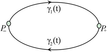
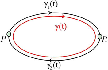
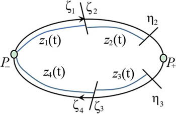
Heteroclinic loop
From
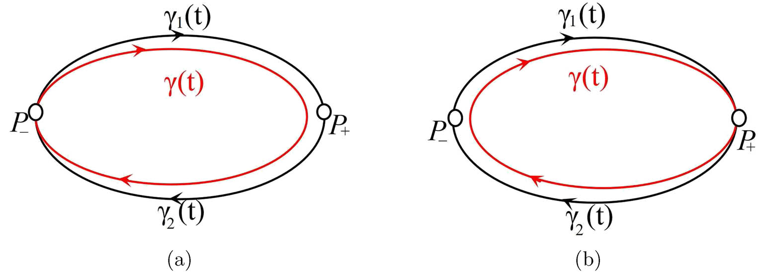
The variational equation of (1.1) along the heteroclinic orbit
Since
for
The structure of this study is organized as follows. In Section 2, we first study the variational equation of (1.1) along the degenerate heteroclinic orbit
2 Preliminaries and main result
2.1 Lin’s method
We give a brief description of the idea of Lin’s method in this section, refer [6] for details. Lin’s method is an analytical tool to deal with heteroclinic loop bifurcation.
We assume that for
By the assumptions, we know that the system has a heteroclinic loop consisting of saddles
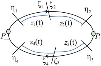
We apply Lin’s method to construct Lin orbits
There are constants
That is, the existence of perodic orbits is equivalent to the existence of
2.2 Exponential dichotomy
Since
By the exponential dichotomy roughness theorem, we know (1.3) has two-side exponential dichotomies on
Lemma 2.1
Assume that (H5) and (H6) hold. There exists a fundamental matrix solution
where constants
where
Moreover,
For the variational equation
we have analogous two-side exponential dichotomies on
Lemma 2.2
Assume that (H5) and (H6) hold. There exists a fundamental matrix solution
where
Moreover,
2.3 Statement of the main result
Before presenting the main result, we introduce some notations. Let
where
for
Let
for
Let
for
Further, we let
where
Our main result can be stated as follows.
Theorem 1
Assume that (H1)–(H5) hold. Let
and
is a nonsingular
The proof establishing the existence of a periodic solution bifurcating from the heteroclinic loop
The periodic solution bifurcated from heteroclinic loop
The homoclinic solution bifurcated from heteroclinic loop
3 Proof of Theorem 1
For the proof of the conclusion of Theorem 1, we apply Lin’s method for constructing Lin orbits
3.1 Periodic solution bifurcated from heteroclinic loop
Γ
In this section, our objective is to find periodic solution near the unperturbed heteroclinic loop
We define functions
and
where
uniformly with respect to
For
Then,
with
and
By the definition of the function
Let
Lemma 3.1
For any
Let
For any
Lemma 3.2
Given
Proof
For given
Next we will prove that the above integral equation has a continuous solution. Using the equation
Let the constants
for
With this choice of
For any
for
for
For any
for
Thus, we conclude that
The proof is complete.□
If we can seek some
By the definition of
Next we will seek some
From
From
and
In (3.13), taking
where (2.3) and (2.5) are used to ensure the existence of the limit,
From (3.15), we can solve
Then, there exists
Substituting
Lemma 3.3
Assume
for
Next we will give a sufficient condition for the existence of zeros of (3.16) and (3.17). Based on
By the properties of
uniformly with respect to
and by
hence
where
where
where
for
Let
It follows from the definition of the projection
Hence,
where
where
Lemma 3.4
If there exists
Proof
Let
By the definition of
From (3.21) and (3.22), it is easy to check that
Let
Note that
for
for
For any
which implies that
For
Hence, for any
By the definition of
where
By transformations (3.1) and (3.2), we know that for
where
where
Next we seek homoclinic solution near the unperturbed heteroclinic loop
3.2 Homoclinic solution bifurcated from heteroclinic loop
Γ
In this section, we consider the homoclinic solution bifurcated from heteroclinic loop
Define a function
where
uniformly with respect to
Then,
with
and
With regard to
By the definition of the function
with the norm
For any
Lemma 3.5
Given
We only need to show that the definitions of
and
are convergent. Hence the definition of
Here
From
From
In (3.39), taking the
where (2.3) and (2.5) are used to make sure the existence of the limit, and
From (3.40), we can solve
Then, there exists
Substituting
Lemma 3.6
Assume
for
Next, in a similar way, we give a sufficient condition for the existence of zeros of (3.41) and (3.42) and obtain the same bifurcation function as (3.21). Hence, the zeros of the bifurcation function correspond to the existence of a homoclinic solution for the perturbed equation. So, under the conditions of Lemma 3.4, we know that for
where
In summary, we have demonstrated the perturbed equation (1.2) has periodic or homoclinic solution
Acknowledgement
We are grateful to the anonymous referees for the constructive comments on the manuscript.
-
Funding information: This work was supported by the National Natural Science Foundation of China (Grant No. 11801343).
-
Author contributions: Both authors equally contributed to this work. Both authors read and approved the final manuscript.
-
Conflict of interest: The authors state no conflict of interest.
-
Data availability statement: All relevant data analyzed during this study are included in this published article.
References
[1] A. J. Homburg and B. Sandstede, Homoclinic and heteroclinic bifurcations in vector fields, Chapter 8 in Handbook of Dynamical Systems, vol. 3, Elsevier, Amsterdam, 2010. 10.1016/S1874-575X(10)00316-4Suche in Google Scholar
[2] C. Bonatti, L. J. Daz, and M. Viana, Dynamics Beyond Uniform Hyperbolicity: A Global Geometric and Probabilistic Perspective, Springer-Verlag, Berlin, 2004. Suche in Google Scholar
[3] K. H. Alfsen, and J. Frøyland, Systematics of the Lorenz model at σ=10, Phys. Scr. 31 (1985), 15–20, DOI: https://doi.org/10.1088/0031-8949/31/1/003. 10.1088/0031-8949/31/1/003Suche in Google Scholar
[4] W. Zhang, B. Krauskopf, and V. Kirk, How to find a codimension-one heteroclinic cycle between two periodic orbits, Discrete Contin. Dyn. Syst. 32 (2012), 2825–2851, DOI: https://doi.org/10.3934/dcds.2012.32.2825. 10.3934/dcds.2012.32.2825Suche in Google Scholar
[5] S. N. Chow, J. K. Hale, and J. Mallet-Parret, An example of bifurcation to homoclinic orbits, J. Differential Equations 37 (1980), 551–573, DOI: https://doi.org/10.1016/0022-0396(80)90104-7. 10.1016/0022-0396(80)90104-7Suche in Google Scholar
[6] X. B. Lin, Lin’s method, Scholarpedia 3 (2008), no. 9, 6972, DOI: https://dx.doi.org/10.4249/scholarpedia.6972.10.4249/scholarpedia.6972Suche in Google Scholar
[7] J. Knobloch, Lin’s method for discrete dynamical systems, J. Difference Equ. Appl. 6 (2000), no. 5, 577–623, DOI: https://doi.org/10.1080/10236190008808247. 10.1080/10236190008808247Suche in Google Scholar
[8] H. P. Krishnan, Uniqueness of rapidly oscillating periodic solutions to a singularly perturbed differential-delay equation, Electron. J. Differential Equations 2000 (2000), no. 56, 1–18. Suche in Google Scholar
[9] B. E. Oldeman, R. A. Champneys, and B. Krauskopf, Homoclinic branch switching: A numerical implementation of Lin’s method, Internat. J. Bifur. Chaos Appl. Sci. Engrg. 13 (2003), no. 10, 2977–2999, DOI: https://doi.org/10.1142/S0218127403008326. 10.1142/S0218127403008326Suche in Google Scholar
[10] C. Zhu, From homoclinics to quasi-periodic solutions for ordinary differential equations, Proc. Roy. Soc. Edinburgh Sect. A 145 (2015), no. 5, 1091–1114, DOI: https://doi.org/10.1017/S0308210515000189. 10.1017/S0308210515000189Suche in Google Scholar
[11] C. Zhu and B. Long, The periodic solution bifurcated from homoclinic orbit for a coupled ordinary differential equations, Math. Methods Appl. Sci. 40 (2017), no. 8, 2834–2846, DOI: https://doi.org/10.1002/mma.4200. 10.1002/mma.4200Suche in Google Scholar
[12] C. Zhu and W. Zhang, Multiple chaos arising from single-parametric perturbation of a degenerate homoclinic orbit, J. Differential Equations 268 (2020), no. 10, 5672–5703, DOI: https://doi.org/10.1016/j.jde.2019.11.024. 10.1016/j.jde.2019.11.024Suche in Google Scholar
[13] S. N. Chow, B. Deng, and D. Terman, The bifurcation of homoclinic and periodic orbits from two heteroclinic orbits, SIAM J. Math. Anal. 21 (1990), no. 1, 179–204, DOI: https://doi.org/10.1137/0521010. 10.1137/0521010Suche in Google Scholar
[14] J. D. M. Rademacher, Homoclinic orbits near heteroclinic cycles with one equilibrium and one periodic orbit, J. Differential Equations 218 (2005), no. 2, 390–443, DOI: https://doi.org/10.1016/j.jde.2005.03.016. 10.1016/j.jde.2005.03.016Suche in Google Scholar
[15] Y. Jin, D. Zhang, N. Wang, and D. Zhu, Bifurcations of twisted of fine heteroclinic Loop for high-dimensional systems, J. Appl. Anal. Comput. 13 (2023), no. 5, 2906–2921, DOI: https://doi.org/10.11948/20230052. 10.11948/20230052Suche in Google Scholar
[16] D. M. Zhu and Y. Sun, Homoclinic and periodic orbits arising near the heteroclinic cycle connecting saddle-focus and saddle under reversible condition, Acta Math. Sin. (Engl. Ser.) 23 (2007), no. 8, 1495–1504, DOI: https://doi.org/10.1007/s10114-005-0746-7. 10.1007/s10114-005-0746-7Suche in Google Scholar
[17] I. S. Labouriau and A. A. P. Rodrigues, Dense heteroclinic tangencies near a Bykov cycle, J. Differential Equations 259 (2015), no. 11, 5875–5902, DOI: https://doi.org/10.1016/j.jde.2015.07.017. 10.1016/j.jde.2015.07.017Suche in Google Scholar
[18] J. Knobloch, J. S. W. Lamb, and K. N. Webster, Using Lin’s method to solve Bykov’s problems, J. Differential Equations 257 (2014), no. 8, 2984–3047, DOI: https://doi.org/10.1016/j.jde.2014.06.006. 10.1016/j.jde.2014.06.006Suche in Google Scholar
[19] B. Long and S. S. Xu, Persistence of the heteroclinic loop under periodic perturbation, Electron. Res. Arch. 31 (2023), no. 2, 1089–1105, DOI: https://doi.org/10.3934/era.2023054. 10.3934/era.2023054Suche in Google Scholar
[20] F. Chen, A. Oksasoglu, and Q. Wang, Heteroclinic tangles in time-periodic equations, J. Differential Equations 254 (2013), no. 3, 1137–1171, DOI: https://doi.org/10.1016/j.jde.2012.10.010. 10.1016/j.jde.2012.10.010Suche in Google Scholar
[21] I. S. Labouriau and A. A. P. Rodrigues, Bifurcations from an attracting heteroclinic cycle under periodic forcing, J. Differential Equations 269 (2020), no. 5, 4137–4174, DOI: https://doi.org/10.1016/j.jde.2020.03.024. 10.1016/j.jde.2020.03.024Suche in Google Scholar
[22] I. S. Labouriau and A. A. P. Rodrigues, Periodic forcing of a heteroclinic network, J. Differential Equations 35 (2023), 2951–2969, DOI: https://doi.org/10.1007/s10884-021-10054-w. 10.1007/s10884-021-10054-wSuche in Google Scholar
[23] X. Sun, Exact bound on the number of limit cycles arising from a periodic annulus bounded by a symmetric heteroclinic loop, J. Appl. Anal. Comput. 10 (2020), no. 1, 378–390, DOI: https://doi.org/10.11948/20190294. 10.11948/20190294Suche in Google Scholar
[24] Y. Xiong and G. Hu, Heteroclinic loop bifurcations by perturbing a class of Z2-equivariant quadratic switching Hamiltonian systems with nilpotent singular points, J. Math. Anal. Appl. 532 (2024), no. 2, 127977, DOI: https://doi.org/10.1016/j.jmaa.2023.127977. 10.1016/j.jmaa.2023.127977Suche in Google Scholar
[25] B. Long and Y. Yang, Applying Lin’s method to constructing heteroclinic orbits near the heteroclinic chain, Math. Methods Appl. Sci. 47 (2024), no. 12, 10235–10255, DOI: https://doi.org/10.1002/mma.10118. 10.1002/mma.10118Suche in Google Scholar
[26] W. Coppel, Dichotomies and Stability Theory, Springer-Verlag, Berlin, 1978. 10.1007/BFb0067780Suche in Google Scholar
[27] K. J. Palmer, Exponential dichotomies and transversal homoclinic points, J. Differential Equations 55 (1984), no. 2, 225–256, DOI: https://doi.org/10.1016/0022-0396(84)90082-2. 10.1016/0022-0396(84)90082-2Suche in Google Scholar
[28] M. Feckan and J. Gruendler, Bifurcation from homoclinic to periodic solutions in singular ordinary differential equations, J. Math. Anal. Appl. 246 (2000), no. 1, 245–264, DOI: https://doi.org/10.1006/jmaa.2000.6791. 10.1006/jmaa.2000.6791Suche in Google Scholar
© 2025 the author(s), published by De Gruyter
This work is licensed under the Creative Commons Attribution 4.0 International License.
Artikel in diesem Heft
- Special Issue on Contemporary Developments in Graphs Defined on Algebraic Structures
- Forbidden subgraphs of TI-power graphs of finite groups
- Finite group with some c#-normal and S-quasinormally embedded subgroups
- Classifying cubic symmetric graphs of order 88p and 88p 2
- Simplicial complexes defined on groups
- Two-sided zero-divisor graphs of orientation-preserving and order-decreasing transformation semigroups
- Further results on permanents of Laplacian matrices of trees
- Special Issue on Convex Analysis and Applications - Part II
- A generalized fixed-point theorem for set-valued mappings in b-metric spaces
- Research Articles
- Dynamics of particulate emissions in the presence of autonomous vehicles
- The regularity of solutions to the Lp Gauss image problem
- Exploring homotopy with hyperspherical tracking to find complex roots with application to electrical circuits
- The ill-posedness of the (non-)periodic traveling wave solution for the deformed continuous Heisenberg spin equation
- Some results on value distribution concerning Hayman's alternative
- 𝕮-inverse of graphs and mixed graphs
- A note on the global existence and boundedness of an N-dimensional parabolic-elliptic predator-prey system with indirect pursuit-evasion interaction
- On a question of permutation groups acting on the power set
- Chebyshev polynomials of the first kind and the univariate Lommel function: Integral representations
- Blow-up of solutions for Euler-Bernoulli equation with nonlinear time delay
- Spectrum boundary domination of semiregularities in Banach algebras
- Statistical inference and data analysis of the record-based transmuted Burr X model
- A modified predictor–corrector scheme with graded mesh for numerical solutions of nonlinear Ψ-caputo fractional-order systems
- Dynamical properties of two-diffusion SIR epidemic model with Markovian switching
- Classes of modules closed under projective covers
- On the dimension of the algebraic sum of subspaces
- Periodic or homoclinic orbit bifurcated from a heteroclinic loop for high-dimensional systems
- On tangent bundles of Walker four-manifolds
- Regularity of weak solutions to the 3D stationary tropical climate model
- A new result for entire functions and their shifts with two shared values
- Freely quasiconformal and locally weakly quasisymmetric mappings in metric spaces
- On the spectral radius and energy of the degree distance matrix of a connected graph
- Solving the quartic by conics
- A topology related to implication and upsets on a bounded BCK-algebra
- On a subclass of multivalent functions defined by generalized multiplier transformation
- Local minimizers for the NLS equation with localized nonlinearity on noncompact metric graphs
- Approximate multi-Cauchy mappings on certain groupoids
- Multiple solutions for a class of fourth-order elliptic equations with critical growth
- A note on weighted measure-theoretic pressure
- Majorization-type inequalities for (m, M, ψ)-convex functions with applications
- Recurrence for probabilistic extension of Dowling polynomials
- Unraveling chaos: A topological analysis of simplicial homology groups and their foldings
- Global existence and blow-up of solutions to pseudo-parabolic equation for Baouendi-Grushin operator
- A characterization of the translational hull of a weakly type B semigroup with E-properties
- Some new bounds on resolvent energy of a graph
- Carmichael numbers composed of Piatetski-Shapiro primes in Beatty sequences
- The number of rational points of some classes of algebraic varieties over finite fields
- Singular direction of meromorphic functions with finite logarithmic order
- Pullback attractors for a class of second-order delay evolution equations with dispersive and dissipative terms on unbounded domain
- Eigenfunctions on an infinite Schrödinger network
- Boundedness of fractional sublinear operators on weighted grand Herz-Morrey spaces with variable exponents
- On SI2-convergence in T0-spaces
- Bubbles clustered inside for almost-critical problems
- Classification and irreducibility of a class of integer polynomials
- Existence and multiplicity of positive solutions for multiparameter periodic systems
- Averaging method in optimal control problems for integro-differential equations
- On superstability of derivations in Banach algebras
- Investigating the modified UO-iteration process in Banach spaces by a digraph
- The evaluation of a definite integral by the method of brackets illustrating its flexibility
- Existence of positive periodic solutions for evolution equations with delay in ordered Banach spaces
- Tilings, sub-tilings, and spectral sets on p-adic space
- The higher mapping cone axiom
- Continuity and essential norm of operators defined by infinite tridiagonal matrices in weighted Orlicz and l∞ spaces
-
A family of commuting contraction semigroups on
- Pullback attractor of the 2D non-autonomous magneto-micropolar fluid equations
- Maximal function and generalized fractional integral operators on the weighted Orlicz-Lorentz-Morrey spaces
- On a nonlinear boundary value problems with impulse action
- Normalized ground-states for the Sobolev critical Kirchhoff equation with at least mass critical growth
- Decompositions of the extended Selberg class functions
- Subharmonic functions and associated measures in ℝn
- Some new Fejér type inequalities for (h, g; α - m)-convex functions
- The robust isolated calmness of spectral norm regularized convex matrix optimization problems
- Multiple positive solutions to a p-Kirchhoff equation with logarithmic terms and concave terms
- Joint approximation of analytic functions by the shifts of Hurwitz zeta-functions in short intervals
- Green's graphs of a semigroup
- Some new Hermite-Hadamard type inequalities for product of strongly h-convex functions on ellipsoids and balls
- Infinitely many solutions for a class of Kirchhoff-type equations
- On an uncertainty principle for small index subgroups of finite fields