Computational modeling of pitting corrosion
-
Siavash Jafarzadeh
Siavash Jafarzadeh received his BSc (2011) and MSc (2015) degrees in Mechanical Engineering from Isfahan University of Technology, Isfahan, Iran. In 2016, he started his PhD program in Mechanical Engineering and Applied Mechanics at University of Nebraska-Lincoln, USA. His doctoral research is focused on computational modeling of corrosion damage and stress corrosion cracking, using peridynamic theory.
Ziguang Chen received his PhD degree in Mechanical Engineering and Applied Mechanics from University of Nebraska-Lincoln, USA, in 2012. He worked as a postdoctoral researcher in the same university from 2013 to 2017. He is currently a Professor in the Department of Mechanics at Huazhong University of Science and Technology, China.
 and
Florin Bobaru
and
Florin Bobaru
Florin Bobaru received his BS (1995) and MS (1997) degrees in Mathematics and Mechanics from University of Bucharest, Romania, and his PhD (2001) degree in Theoretical and Applied Mechanics from Cornell University, USA. He is currently a Professor and Hergenrader Distinguished Scholar in Mechanical and Materials Engineering at University of Nebraska-Lincoln, USA. He is the main editor of the
Handbook of Peridynamic Modeling (2017).


Abstract
Pitting corrosion damage is a major problem affecting material strength and may result in difficult to predict catastrophic failure of metallic material systems and structures. Computational models have been developed to study and predict the evolution of pitting corrosion with the goal of, in conjunction with experiments, providing insight into pitting processes and their consequences in terms of material reliability. This paper presents a critical review of the computational models for pitting corrosion. Based on the anodic reaction (dissolution) kinetics at the corrosion front, transport kinetics of ions in the electrolyte inside the pits, and time evolution of the damage (pit growth), these models can be classified into two categories: (1) non-autonomous models that solve a classical transport equation and, separately, solve for the evolution of the pit boundary; and (2) autonomous models like cellular automata, peridynamics, and phase-field models which address the transport, dissolution, and autonomous pit growth in a unified framework. We compare these models with one another and comment on the advantages and disadvantages of each of them. We especially focus on peridynamic and phase-filed models of pitting corrosion. We conclude the paper with a discussion of open areas for future developments.
1 Introduction
Pitting corrosion is a particular type of localized corrosion, in which the corrosion rate is higher in some areas compared with others (Jones, 1992; Frankel, 1998; Revie, 2008; Marcus, 2011). Pitting corrosion damage is observed in many alloys which are protected from general corrosion by a passive film on their surface. Some widely used alloys, like stainless steel and aluminum alloys, suffer from pitting corrosion. Corrosion pits with various shapes and forms, some developing “hidden” by a perforated cover, can grow large and contribute to catastrophic failure in engineering structures subjected to mechanical loading: for example, turbine blades (Rani et al., 2017), bridges (National Transportation Safety Board, 2008), pipelines (Zhu et al., 2015), and nuclear power plants (Cattant et al., 2008). Controlled by chemical reactions and influenced across length scales by environmental and mechanical loading conditions, corrosion pits can lead to embrittlement (loss of ductility) and significant reductions in strength (Horner et al., 2011; Co and Burns, 2017; Sheng and Xia, 2017; Li et al., 2018).
With advances in technology in the recent decades, and the substantial increase in computer power, computational models are now capable of utilizing mathematical models to simulate complex multi-physics phenomena with high resolution. Computational simulations, once calibrated and validated against carefully conducted experiments, can expand the reach of experimental investigations to more realistic conditions and to length and time scales difficult to investigate otherwise. Predictive science and engineering happens more and more using computational modeling and simulations.
Pitting corrosion models have been used to predict pit growth in different materials exposed to various environments. Some such models are analytical, and given certain input parameters, they can estimate pit depth in time (Valor et al., 2007; Velázquez et al., 2009; Li et al., 2014). Knowing that failure does not always start from the bottom of a corrosion pit (Turnbull et al., 2010; Huang et al., 2017), more detailed studies are warranted for gaining the ability to predict failure and then design against it. Computational models of corrosion provide a solution here. These models start from mathematical formulations for electro-chemo-mechanical phenomena and use various numerical methods to solve for the progression of the pitting process in more detail: the evolution of pits’ shape and morphology, the concentration of different chemical species inside and outside of the pit, the electric potential distribution over the domain of interest, etc., can all be found using such models. Reaction kinetics at the corrosion front and the transport kinetics of the chemical species inside the pits are usually taken as the basis for these models.
In the past few years, a number of review papers focused on computational modeling (mostly finite-element based) of corrosion (Amaya et al., 2014; Laycock et al., 2014; Liu and Kelly, 2014; Taylor, 2014; Bhandari et al., 2015). In the present review, we focus attention on recent approaches to modeling pitting corrosion, like cellular automata (CA) techniques, peridynamic (PD) formulations, and phase-field (PF) models. We point out and discuss advantages over the more traditional models. This review is not an exhaustive one, but we hope that it will offer a useful starting point for researchers and engineers working on understanding and predicting corrosion damage and, in particular, pitting corrosion.
The paper is organized as follows: we start with a brief discussion of the fundamentals of corrosion kinetics. We then introduce a classification of the models based on how pit propagation is computed in time: classical or “non-autonomous” models (which solve for the corrosion front as a separate step in the solution process) and the more recent “autonomous” models (in which the evolution of the corrosion front is autonomous, e.g. CA, PD, and PF models). These models are reviewed and compared with one another in terms of their strengths and drawbacks. We conclude with a discussion on a number of knowledge gaps and open areas in computational modeling of pitting corrosion and offer some suggestions for future areas of research.
2 Corrosion kinetics basics
Corrosion damage is a complex phenomenon (Jones, 1996; Revie, 2008; Marcus, 2011). The study of corrosion problems requires multidisciplinary knowledge, including electrochemistry, metallurgy, thermodynamics, and mechanics. The corrosion damage process generally involves the following: dissolution of the material due to electrochemical reactions with an electrolyte at the metal surface, transport of the dissolved metal atoms in the environment, and the mechanical degradation (loss of ductility, damage) of the material caused by the corrosion. The most relevant scale for understanding pitting corrosion during initiation and early-stage propagation is the micrometer to millimeter scale, and all of the simulation models reviewed in this paper focus on this scale. Simulations in the micrometer to millimeter scale allow one to understand the evolution of pit morphologies, the growth rate, and, in some cases, the corresponding mechanical degradation induced by the corrosion process. Atomistic models for corrosion processes, like molecular dynamic models that study the details of chemical reactions, are not reviewed in this paper. For a discussion of that topic, please see Taylor and Marcus (2015), Marcus and Maurice (2017), and Verma et al. (2018).
Basics for pit growth models include the dissolution kinetics at the corrosion front and the transport kinetics of species inside the electrolyte. These are briefly reviewed next.
2.1 Corrosion reaction kinetics
Pit growth in localized corrosion in metals exposed to aqueous solution can be reduced to the anodic reaction at the pit surface, since it is the reaction responsible for dissolution. The generic form of the anodic reaction can be expressed as
where M(s) denotes a generic metal atom in the solid state, M(aq)z+ is the dissolved metal ion with the charge number z in the aqueous solution, and e− refers to an electron. Figure 1 shows the schematic of localized metal dissolution by the anodic reaction in the presence of the electrolyte.
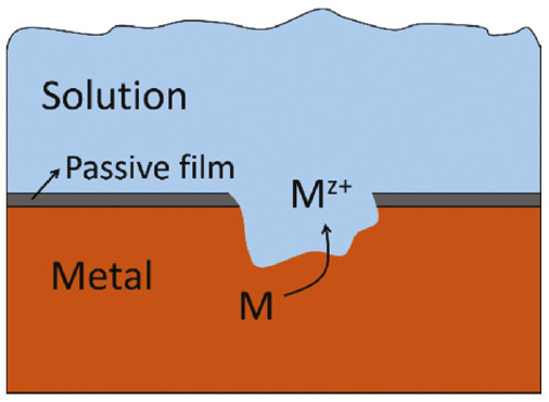
Schematic of anodic dissolution of some metal atom (M) and its dissolved state in the solution with +z charge number: Mz+.
The produced electrons in the anodic reaction travel in the solid metal, reach out the surface at a point (usually outside of the pit), and participate in the cathodic reactions. The results of the cathodic reactions are corrosion products (H2 gas, precipitated solid products like rust in corrosion of iron-based alloys, etc.). Except for a few models like one mentioned in Section 3.2.2, most of the computational models for pitting corrosion only focus on the anodic reaction rate which determines the metal dissolution and the pit growth rate. Based on Arrhenius equation for reaction rate which originates from experimental observations and thermodynamic analysis, the anodic reaction rate can be expressed by (Bard et al., 1980)
where ia is the anodic current density, η is the over potential, F is Faraday’s constant, R is the gas constant, T is the absolute temperature, α is the transfer coefficient (a scalar between 0 and 1), and i0 is the exchange current density associated with zero over potential. η can be expressed as Eapp−Ee where Eapp is the applied potential and Ee is the equilibrium potential.
Note that the anodic current density (iα) scales linearly with the molar dissolution flux (Jdiss) at the corrosion front via Faraday’s law (Bard et al., 1980):
Note that the bold notation is used here when referring to a vector-valued quantity.
When the corrosion rate only depends on the anodic reaction and follows Eq. (2), the corrosion regime is called activation-controlled. The corrosion rate also can depend on other factors such as the transport kinetics of ions in the electrolyte (see next section).
In certain cases, material microstructure heterogeneities (such as crystallographic orientation, grains, grain boundaries, twins, etc.) can have a significant influence on the pit shape and propagation rate (Liu et al., 2008a; Shahryari et al., 2009). Models that aim to address microstructural effects usually use specific reaction kinetics for each phase of the microstructure in the solid domain (Chen and Bobaru, 2015; Mai et al., 2016; Jafarzadeh et al., 2018a).
2.2 Transport kinetics in the electrolyte
When the reaction rate is higher than the diffusion rate in the electrolyte, the dissolved ions Mz+ accumulate near the corroding surface, and once their molar concentration C, reaches the saturation value Csat, the solution cannot sustain higher amount of Mz+. The excess of the ions would precipitate as salt molecules and form a salt layer (Isaacs et al., 1995). Such condition is likely to occur at the pit bottom. The salt layer thickness increases until the potential drop through the thickness balances the dissolution rate with the diffusion rate in the electrolyte. In such condition, the corrosion rate is not controlled by the applied potential but by the diffusion rate inside the electrolyte (Isaacs et al., 1995). This corrosion regime is referred to as the diffusion-controlled mode. Figure 2 shows a schematic description of diffusion-controlled corrosion in comparison with the activation-controlled regime. In Figure 2B, Jtrans is the transport molar flux near the corrosion front (which depends on the diffusivity in the electrolyte and the concentration gradient).
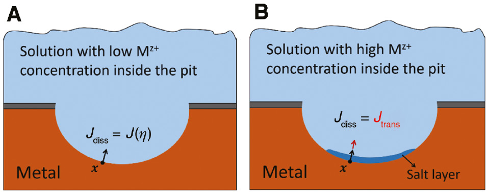
Schematic of metal (M) anodic dissolution in pitting corrosion under (A) activation-controlled and (B) diffusion-controlled corrosion regimes.
Diffusion-controlled corrosion is only one example that points out the importance of transport kinetics inside the solution. Ion transportation in the pit can affect the corrosion rate by modifying the electric potential distribution in the solution, cathodic reactions, formation of corrosion products, etc.
Conservation of mass leads to Eq. (4), which is the general equation used to address the transport of species in the solution (Bard et al., 1980; Sharland et al., 1989):
In Eq. (4), Ci is the molar concentration of ith species, Ji is its molar flux, t is time, and Bi is the reaction term, i.e. a source/sink term for production/depletion of the species.
Nernst-Plank equation is commonly used to describe the transport flux of chemically charged species (Bard et al., 1980). In this equation, the ionic flux in Eq. (4) depends on the gradient of ion concentration (Fick’s law of diffusion), the electric field (electromigration), and the flow in the liquid medium (convection). According to this equation, the molar flux can be expressed as
where Di is a diffusion coefficient of the ith species (assumed to be constant in most models, but in general they could vary with location), v is the velocity, and φ is the electric potential. On the right-hand-side of Eq. (5), the first term is the diffusion flux, the second term represents the electromigration flux, and the third term expresses the advection flux. Equation (5) can be further simplified given the typical physical conditions relevant in a corrosion pit. For example, the convection term can be ignored. For models that include the electromigration term, an additional equation is required in order to find the electric potential φ. Commonly used for this purpose is the Poisson-type equation for φ (Sharland et al., 1989; Tsuyuki et al., 2018), which, in the case of negligible charge density compared with electric permittivity of the electrolyte, reduces to the electro-neutrality equation (Sharland et al., 1989; Xiao and Chaudhuri, 2011):
Most of the computational models for pitting corrosion are directly based on Eqs. (2)–(6) or use alternative formulations to describe the same kinetics (see Section 1).
3 Computational models for pitting corrosion
In this review, we classify the computational models for pitting corrosion in two main categories, according to how the evolution of the corrosion front is computed: non-autonomous models and autonomous models. Non-autonomous models use numerical methods like finite element method (FEM) to solve the transport equation, Eq. (4), over the pit area/volume. They employ techniques to model, separately, the motion of the corrosion front and, thus, the evolution of the pit domain. Autonomous models in comparison use mathematical formulations that describe the dissolution/transport kinetics together with the process of pit propagation (e.g. PD models and PF models) or use discrete approaches that mimic dissolution, transport, and propagation processes (e.g. the CA technique).
3.1 Non-autonomous models
In this section we review non-autonomous (classical) models which use the FEM to solve the transport equations and a moving boundary technique for the evolution of pit growth.
One of the first attempts at numerical modeling of pitting corrosion (Sharland et al., 1989) used the FEM to solve Eq. (4) considering diffusion, reaction, and electromigration of chemical species (Fe2+, H+, OH−) in Eq. (5), inside a rectangular pit, for corrosion in carbon steel (Sharland, 1988; Sharland and Tasker, 1988). This model ignores the pit propagation process and focuses on the transport inside a fix domain (fix pit geometry). A similar model (Walton, 1990) is solved using the finite difference method (FDM), instead of the FEM, by (Walton et al., 1996). Nonetheless, propagation is an essential part for a practical pitting corrosion model and should not be ignored. In the rest of the models reviewed below, the propagation process is included.
Because the exact distribution of the electric potential inside a corrosion pit is not as critical as in some other types of corrosion (e.g. galvanic corrosion), it is reasonable to ignore from Eq. (5), the electromigration term, in addition to the neglected convection term. This is done by most computational models in the published literature. Consequently, assuming constant coefficients (Di), Eqs. (4) and (5) reduce to the classical Fick’s law of diffusion:
where ∇2 denotes the Laplacian operator. Note that if the electric potential distribution significantly varies along the pit surface, or the electromigration has notable contribution to mass transfer, then it is necessary to also account for the contributions from electromigration and the potential field (which needs to be solved for). In addition, if the pit is large and has an open mouth, and the bulk solution outside the pit is not stationary, one needs to include a convective term.
A notable development in FEM modeling of pitting corrosion is the Laycock and White’s (LW) model (Laycock et al., 1998). In this model, the diffusion of the dissolved metal ions is considered in an axisymmetric domain. Diffusion-controlled corrosion regime is assumed over the domain. This leads to imposing the saturation value for concentration of metal ions in the solution (Csat) as a Dirichlet-type boundary condition on the pit boundary when solving Eq. (7) with the FEM.
For propagation of the pit, the flux at the boundary is evaluated after solving the diffusion equation, and, from the conservation of mass principle, the propagation velocity vector is computed at each boundary node:
In Eq. (8), vb is the velocity of point x on the pit boundary, Jdiss is the dissolution flux at the boundary, and M and ρ are respectively the molar mass and the mass density of the solid bulk. Using the boundary velocity (Laycock et al., 1998), calculate the new position for the boundary nodes for the next time step, and after remeshing the updated domain, the problem is solved at the new time step. The current density is easily calculated from Jdiss using Eq. (3) (Faraday’s law).
The LW model can also simulate the formation of perforated (lacy) covers in pitting corrosion of stainless steel. The perforations occur due to a sequence of recurring events: passivation of the pit surface near its mouth, continuation of corrosion underneath the passivated region (undercutting), and breaking/perforating the passive layer on the surface by dissolution and osmotic pressure (Pistorius and Burstein, 1992; Tian et al., 2014). To model formation of lacy covers, Laycock et al. (1998) used a passivation criterion. They considered a critical concentration of metal ions in the solution (Ccrit), below which the corroding surface would passivate. Figure 3 shows the axisymmetric simulation results with this FEM model.
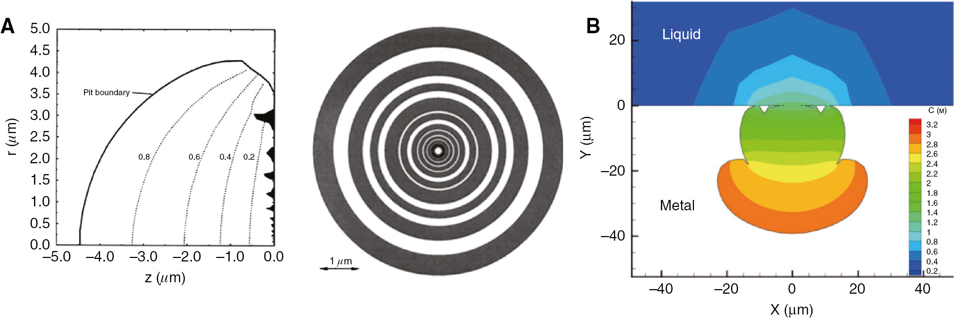
Simulations of pitting corrosion in stainless steel using Laycock and White’s model: (A) half of the pit cross section, and top view of the formed lacy covers in an axisymmetric domain (Laycock et al., 1998). (B) Cross section of a pit grown under galvanostatic conditions (Krouse et al., 2014). The colors represent the metal ion concentration.
The LW model has been further extended in a number of studies (Laycock and White, 2001; Ghahari et al., 2011; Krouse et al., 2014). Instead of enforcing the constant concentration on the pit boundary, these studies considered a concentration-dependent dissolution flux on the corroding boundary as a Neumann-type boundary condition. With this modification, the diffusion-controlled regime could be modeled where the salt layer is likely to form, and the activation-controlled regime takes place over the rest of the pit boundary.
This model has been utilized for simulating pit growth under both potentiostatic and galvanostatic conditions (Laycock and White, 2001; Krouse et al., 2014). Potentiostatic condition refers to the case in which the applied potential is fixed during the pitting process, while the total current increases as the pit grows in time and the corroding area enlarges. In contrast, galvanostatic condition refers to the case in which pitting occurs under constant value of total current. In this condition, the potential decreases as the pit grows because as the corroding area expands, less current density is required to keep the total current constant, which, in turn, results in decreasing potential value in time. Note that these conditions can be controlled in laboratory experimental conditions. In real corrosion problems, the actual conditions may be closer to one or the other. For example, pit growth in a metal immersed in an electrolyte happens in conditions closer to the potentiostatic case, with the global potential being near the pitting potential. Note that the local potential inside the pit may be significantly different from the associated pitting potential because the local chemistry significantly differs inside the pit. For atmospheric corrosion conditions, the case is closer to galvanostatic state, since the cathodic reaction is limited by the thickness of the thin moisture layer formed on the metal surface, which consequently limits the anodic dissolution rate to a nearly fixed value.
These LW-based models, implemented for axisymmetric domains, lead to an evolution of the pit shape with the experimentally observed characteristics of pitting in stainless steels, such as shallow dish-shaped pits with lacy cover on the top, and in certain cases, secondary pits at the pit bottom (Krouse et al., 2014). The model has also been verified against experiments in terms of distribution of the current density on the pit boundary (Laycock et al., 1998; Laycock and White, 2001; Ghahari et al., 2011; Krouse et al., 2014). However, when compared to actual time evolution of pit shapes and morphologies, the model is less reliable in matching experimental observations (Ghahari, 2012). One reason is that the particular relationship used in the model to describe the current density in terms of the concentration of metal ions at the pit surface is shown to differ from experimentally measured values (Ghahari, 2012).
In another study (Xiao and Chaudhuri, 2011), FEM is used to solve Eq. (4), considering the diffusion and electromigration terms expressed in Eq. (5), combined with the electro-neutrality shown as Eq. (6). In this study, the partial differential equation (PDE) is solved with the COMSOL multiphysics software. The moving boundary model for pit growth is implemented in a separate MATLAB program. Considering electromigration allows for simulating pit growth around an inclusion at the metal surface as a micro-galvanic corrosion case. In addition, simulations with this axisymmetric model are used to construct 3D pH-potential diagrams for a representative Al alloy system. However, to the best of our knowledge, this model has not been validated against any experimental data.
The above-mentioned FEM models of pitting corrosion require remeshing of the domain (the growing pit) at each time step. FEM models that use remeshing for solving moving boundary problems introduce extra complexity in computations, making these approaches highly inefficient in 3D (Marzban, 2018). Some recent studies (Duddu, 2014; Vagbharathi and Gopalakrishnan, 2014) employ the level set method in combination with the extended finite element method (XFEM) to update the pit boundary in a fixed, pre-discretized domain (see Figure 4), while the corrosion front moves over this mesh. These studies provided quantitative validations for 2D pit growth in stainless steel, under intact or perforated passive films. In contrast with the LW model, however, the lacy cover in Duddu (2014) and Vagbharathi and Gopalakrishnan (2014) is imposed as a pre-determined boundary condition.
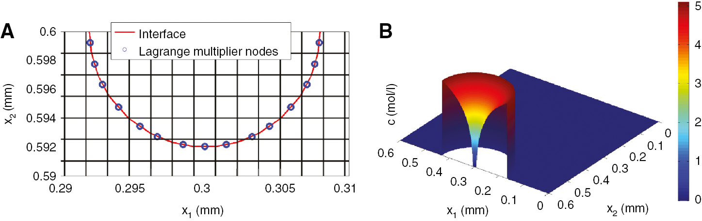
A non-autonomous model that avoids remeshing by using XFEM and level-set method for simulating pit growth over a fixed mesh. (A) Pit boundary moves over the mesh and possesses an independent discretization, shown as Lagrange multiplier nodes. (B) A 3D plot of concentration of metal ions in a 2D simulation of a pit. From Duddu (2014).
Solving transport kinetics with the XFEM combined with moving boundary techniques like the level-set method results in pitting corrosion models that reduce the remeshing problem; note that the corrosion front itself may require some remeshing. However, computing the propagating pit boundary as a moving boundary condition introduces extra computational effort, since now, in addition to solving the PDEs inside the domain, one needs to solve a separate PDE for the evolution of the level set. In the next section we cover other types of models in which the motion of the metal-electrolyte interface is solved directly from the original governing equations, with minimal additional conditions.
3.2 Autonomous models
In this section we review some of the more recent models in which the pit growth is autonomous. Although these models are very different in the way they treat the basic problem, they share among them the autonomous evolution of the corrosion front (driven by a phase change) provided as a direct solution for the main formulation of the corrosion problem. Four types of such models are listed here: a finite volume approach, the CA technique, the PD formulations, and PF models.
The model based on finite volume approach (Scheiner and Hellmich, 2007, 2009) modifies the discretized diffusion equation by including a phase-change strategy that leads to autonomy of corrosion front evolution. CA models for pitting corrosion (Malki and Baroux, 2005; Di Caprio et al., 2011; Stafiej et al., 2013; Van der Weeën et al., 2014; Rusyn et al., 2015; Pérez-Brokate et al., 2016) are discrete models that provide autonomous pit growth based on certain state-transition rules stemming from chemical reactions and transport of chemical species. The autonomous evolution of the corrosion front in PD models of pitting corrosion (Chen and Bobaru, 2015; Chen et al., 2016; De Meo and Oterkus, 2017; Jafarzadeh et al., 2018a,b, 2019a,c) is a result of coupling diffusion of metal ions, phase change due to dissolution at the corrosion front, and mechanical damage near the corroding surface. The model captures changes in structural (damage) and mechanical properties (different elastic modulus, and porosity) taking place at the electrolyte-bulk interface and their influence on corrosion evolution and stress corrosion cracking. This type of nonlocal model leads to a diffuse layer at the pit boundary which happens to match well the experimentally observed microstructure in several alloys (Li et al., 2016, 2018; Badwe et al., 2018; Vallabhaneni et al., 2018; Yavas et al., 2018). PF models of pitting corrosion (Mai et al., 2016; Ansari et al., 2018; Chadwick et al., 2018; Mai and Soghrati, 2018; Nguyen et al., 2018; Tsuyuki et al., 2018) also use a diffuse region instead of a mathematically sharp transition between the electrolyte and the metal, and the governing equations in this case consist of two coupled PDEs in which the “thickness” of the diffuse layer introduces a length scale in the model. All these models are discussed in detail below.
3.2.1 A finite volume approach
Scheiner and Hellmich proposed a model based on the finite volume method (FVM) and a simple scheme (based on a concentration-dependent phase definition) for advancing the corrosion front to simulate pitting corrosion (Scheiner and Hellmich, 2007, 2009). A brief description of the model is given below.
In this model, the domain consists of two main phases: solid phase and liquid phase, where the liquid domain includes the propagating pit. After discretization of the domain with hexagonal volume cells (in 2D with unit thickness), two additional phases are defined for cells at the pit boundary: (1) the electrode-boundary cells (liquid cells in contact with at least one solid cell) and (2) the dissolving solid cells (solid cells in contact with at least one electrode-boundary cell). The rest of the solid cells are called inert solid. Figure 5 shows the volume cells and the four defined phases near the corroding surface. The finite volume discretization of the classical diffusion equation [Eq. (7)] for molar concentration of the dissolved metal ions (Mz+) is solved in the liquid subdomain, but not over the electrolyte boundary cells. At each time step, the concentration in the “electrolyte-boundary” cells and the “dissolving solid” cells are calculated from summation of the fluxes at all of the cell edges for each cell, with the flux between the dissolving solid and the electrolyte boundary being defined according to the jump condition and mass conservation.
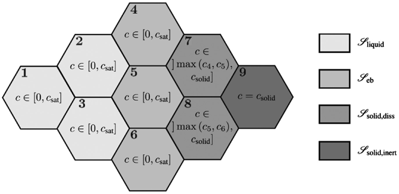
The hexagonal volume cells and the four defined phases near the metal-electrolyte interface in the FVM model by Scheiner and Hellmich (2009).
Validation of the Scheiner and Hellmich (2007) model has been performed against a 2D pit grown in stainless steel, reported in Ernst and Newman (2002). However, in this simulation the model does not capture the formation of lacy covers and uses a pre-determined lacy cover configuration, enforced as piece-wise no-flux/zero-concentration boundary condition on the pit mouth. Figure 6 shows the simulation results presented in (Scheiner and Hellmich, 2007).
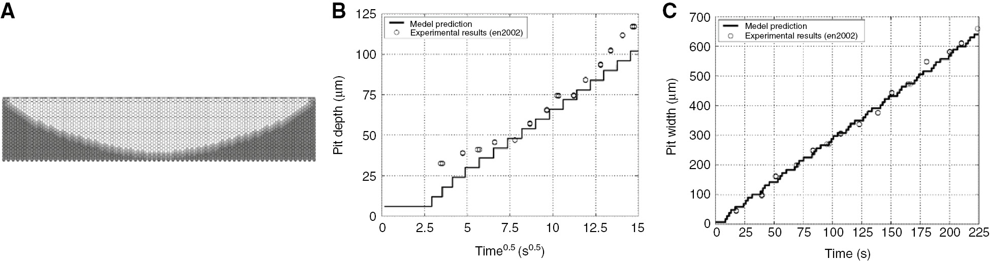
2D simulation of a pit grown in stainless steel by the FVM model (Scheiner and Hellmich, 2007), given the lacy cover as a prescribed boundary condition, and comparison with an experimental pit (Ernst and Newman, 2002): (A) FVM simulated pit shape; (B) pit depth evolution; and (C) pit width evolution.
Although propagation of the pit in this model is autonomous and does not require the explicit tracking of the pit boundary, we note that the thickness of the transition layer (the dissolving solid cells) between the electrolyte and metal is discretization-dependent. Coupling to corrosion-induced damage has not been pursued with this model.
A similar study (Cui et al., 2019) also uses the notion of interaction of nearest-neighbor nodes for solving mass transfer in the liquid and a phase-change criterion of solid nodes adjacent to liquid nodes based on mass conservation. The model uses the Lattice Boltzmann method for mass transfer, which is popular in fluid dynamics (Chen and Doolen, 1998; Rahmati and Niazi, 2012; Rahmati et al., 2012; Rahmati and Niazi, 2014). This model simulates autonomous pit growth, mass transfer of several species in electrolyte, passivation, and corrosion products. However, the paper does not include any verification/validation results. In addition, the phase change in this study requires initialization in the newly transformed nodes which requires extra computation and increases the complexity of the model.
3.2.2 CA models
In CA models, a multi-phase domain consisting of discrete cells with finite states that evolve according to certain local rules is used to simulate the evolution of multi-phase systems. CA techniques have been used for simulating public transportation systems (Chowdhury et al., 2000), spread of forest fires (Encinas et al., 2007), cell growth (Lee et al., 1995), etc. Because CA corrosion models are based on simplified heuristics of chemical reactions in the system, they can capture some effects that the detailed chemistry has on the larger scale (pit-size scale) evolution of the system. Compared to other pitting corrosion models, the CA technique does not involve the PDE-based mathematical formulations and, therefore, leads to relatively simple computational implementations.
Figure 7 shows a schematic diagram of the cellular automaton pitting model (Stafiej et al., 2013). The 2D domain in which the metal and solution are located is discretized into uniform square cells. Each cell is instantiated with a specific state. In this example, the solid phase includes the following: metal, passive, and reactive states. The electrolyte phase can have three different states: alkaline, acidic, and neutral. In addition to the states, each cell also has its own spatial position information, as well as the direction of motion for their states (metal and passivation cells have no motion in this example).
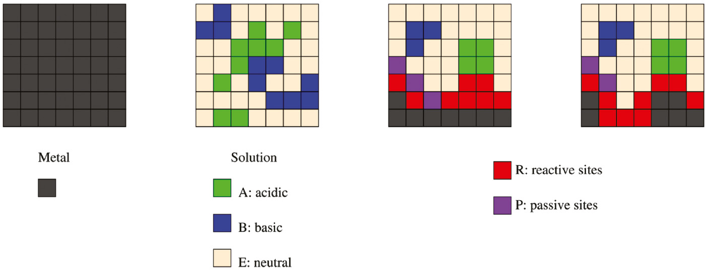
Schematics of a 2D cellular automata model. Six different states are defined for cells in the discrete domain (Stafiej et al., 2013).
In CA models, some basic physical and chemical processes, such as mass transfer, metal dissolution, metal passivation, and repassivation, are qualitatively represented by the interactions and relative state between the cells. For example, chemical reaction kinetics is represented by state change of metal cells with respect to the state of their neighboring liquid cells, which can be acidic, basic or neutral. The transport of states in the electrolyte is modeled by the “random walk” process (Stafiej et al., 2013). The CA models for corrosion differ among them in terms of the materials systems studied, the transition rules enforced, the methods employed to determine the CA model parameters (e.g. the probability of transition of each state to other states), and the dimension (2D or 3D). Figure 8 shows one 2D (A) and one 3D example (B) for CA simulations (Di Caprio et al., 2011; Pérez-Brokate et al., 2016).
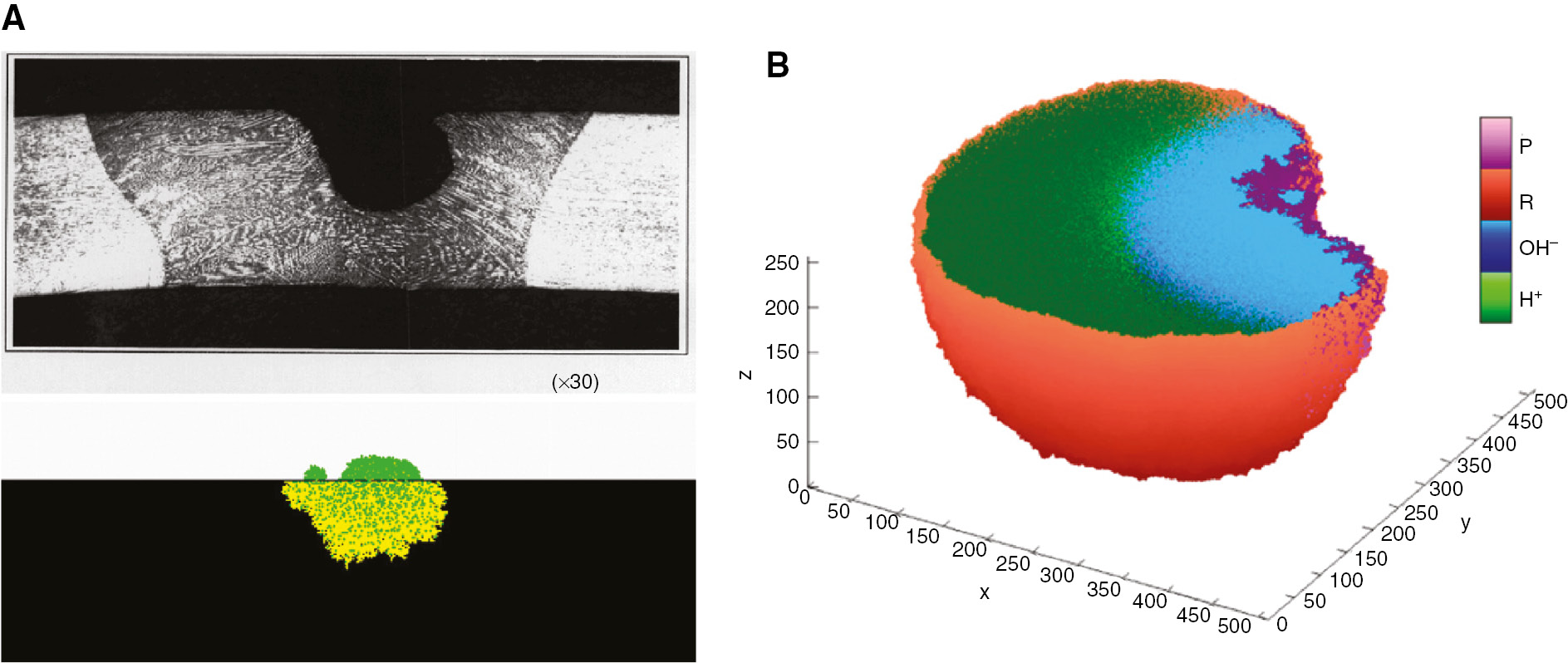
Examples of pitting corrosion simulations by cellular automata models: (A) qualitative comparison of a 2D CA simulation with an experimental pit (Di Caprio et al., 2011); (B) a 3D simulated pit with states and colors being the same as in Figure 7 (Pérez-Brokate et al., 2016).
Reaction-based transition rules of the discrete cell states are a convenient tool to sometimes obtain realistic-looking and stochastic pit morphologies in CA simulations. CA simulations of intergranular corrosion in Di Caprio et al. (2016) suggest that CA is also capable of including alloy microstructure in pitting corrosion. However, the major drawback of this approach is that the time magnitude and spatial sizes (model physical dimensions) are not physical quantities and need to be calibrated for particular transition rules and experimental observation (Van der Weeën et al., 2014; Chuanjie et al., 2019). In addition, the state-transition rules are subjective and difficult to determine for a predictive model. As a result, most CA models only perform parametric studies, without a quantitative comparison with experiments (Malki and Baroux, 2005; Pidaparti et al., 2008; Di Caprio et al., 2011; Stafiej et al., 2013; Pérez-Brokate et al., 2016; Liu et al., 2019). One study that attempts a comparison against experiments (Van der Weeën et al., 2014) solves an inverse problem to better fit the model parameters to various experimental measurements of the corrosion process. This raises questions about the predictive capabilities of the model, since such a procedure is similar to a curve fit of the experimental data. Another study determines the transition rules based on the Pourbaix diagram, and a verification for the effect of pH on pit shape is provided (Rusyn et al., 2015). Again, physical time was not considered in this study. While, in general, CA techniques may replicate some features observed in pitting corrosion and can be useful for qualitative studies of the pitting process, it is still unclear how they can be used for quantitative predictions of pit growth in real time.
3.2.3 PD models
The basic difference between classical models (which model diffusion in the electrolyte domain only) and PD models for corrosion is that, in PD, corrosion is viewed as a type of damage induced in the solid by dissolution, coupled with the diffusion problem in the electrolyte. PD can easily include microstructure and heterogeneities [see Zhang et al. (2018)] by defining appropriate dissolution properties in each phase of the solid (e.g. grains and grain boundaries in alloys). The benefit of such an approach can be far-reaching because this can capture important changes that happen in the solid phase, near the corrosion front, leading to a better understanding of the factors that control the loss of ductility observed in corroded samples (Pantelakis et al., 2000; Chen et al., 2005; Song et al., 2005; Liu et al., 2008b; Zhong et al., 2017; Li et al., 2018). The PD model for corrosion damage couples diffusion of metal ions in the electrolyte, phase change due to dissolution at the corrosion front, and mechanical damage in the corroding layer, offering a more complete description of corrosion damage (Chen and Bobaru, 2015).
The PD formulation was introduced in 2000 (Silling, 2000) as an extension of classical continuum mechanics that can easily deal with discontinuities (such as cracks) developing in the domain (Ha and Bobaru, 2010; Silling and Lehoucq, 2010; Bobaru and Zhang, 2015; Bobaru et al., 2017; Xu et al., 2018). The governing equations in PD as a nonlocal theory are in the form of integro-differential equations (IDEs). In contrast with the PDEs used in the classical local approach of continuum mechanics, IDEs in PD do not require continuity of the unknown function. Consequently, PD can easily model behaviors associated with bodies with evolving discontinuities, discrete particles, all within a unified framework (Silling and Lehoucq, 2010; Bobaru et al., 2017). While PD models have been primarily used in fracture and damage mechanics (Chen et al., 2019; Behzadinasab et al., 2018; Bobaru et al., 2018; Mehrmashhadi et al., 2019), the theory has been extended to other areas as well, including diffusion phenomena like heat/mass transfer (Bobaru and Duangpanya, 2010, 2012; Oterkus et al., 2014; Zhao et al., 2018).
Note that PD is a nonlocal theory, meaning that the material behavior at each point depends on interactions of that point with not only nearest-neighbor points. Nonlocal approaches provide a convenient way to model the evolution of material damage according to changes/loss of interactions between points. In general, nonlocal theories are considered to be better fit for modeling damage-related problems compared to classical local continuum theories because they can capture physical features of damage which are difficult to model with local models, such as small-scale heterogeneities, distributed damage, etc. (Bažant, 1991; Bažant and Jirásek, 2002; Bobaru and Zhang, 2015).
Corrosion is a type of damage that progresses in the material by dissolution, and it influences the mechanical behavior in some significant ways (Pantelakis et al., 2000; Chen et al., 2005; Song et al., 2005; Liu et al., 2008b; Zhong et al., 2017; Li et al., 2018). Recent experiments report a small-scale distributed damage in a thin (micrometer-scale) layer near the corrosion front referred to as the “diffuse corrosion layer” (DCL), with degraded mechanical properties and gradual changes in chemical composition (Li et al., 2016, 2018; Badwe et al., 2018; Vallabhaneni et al., 2018; Yavas et al., 2018). The nonlocality of PD models allows to easily capture the distributed damage in the DCL and its evolution (Chen and Bobaru, 2015; Jafarzadeh et al., 2018b).
The DCL found in the experiments mentioned above (performed on a number of material systems, like Mg and Al alloys) can be several micrometers thick. In certain cases, this may be sufficient to allow microcracks to easily grow in it, in a brittle fashion. Since the DCL is seamlessly attached to the bulk, and the properties change gradually, these cracks can grow into the bulk and lead to significant loss of overall ductility in the structure. In Li et al. (2018) it was shown that the DCL’s influence on loss of ductility is independent from that caused by hydrogen embrittlement (HE), and it can affect it as strongly as HE, if not more. If the physical properties of the affected layer are inserted in the PD model together with other mechanisms, such as HE, then it may be possible to develop a predictive tool for assessing service life and reliability of materials and structures (under mechanical loading) in corrosive environments.
In PD, each material point x interacts with other material points in its neighborhood Hx shown in Figure 9. This neighborhood is called the horizon region, and its radius, denoted by δ, is called the horizon size. The objects that carry the interactions between material points are called “bonds”. In its simplest (bond-based) mechanical formulation, the PD bonds are analogous to elastic springs (linear or nonlinear) that connect material points. In the PD formulation for diffusion-type problem, these bonds are analogous to pipes that carry mass/heat, and they are characterized by a certain diffusivity parameter. The diffusivity for diffusion bonds is called micro-diffusivity and is denoted by k. In a homogeneous material, micro-diffusivities can be calculated from the classical diffusivity D, used in the classical diffusion equation (Eq. (7)) (Bobaru and Duangpanya, 2012; Zhao et al., 2018).
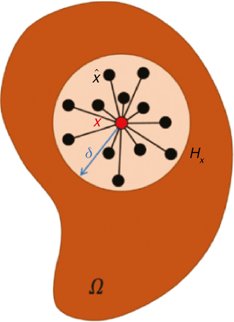
Schematic of a peridynamic domain (Ω): a generic point x interacts with the material points
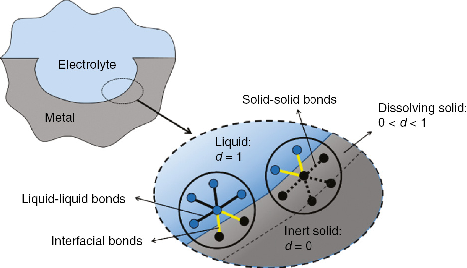
The mechanical damage (d) in PD theory is represented by a scalar-valued quantity stored at the material points and computed based on the number of broken bonds relative to the number of total bonds for that point. This quantity ranges from 0 to 1, with d=1 corresponding to a point which has lost all of its mechanical bonds, and d=0 corresponding to the case when all bonds connecting to x are intact.
Based on the concept of mechanical damage in PD solid mechanics, Chen and Bobaru (2015) introduced PD corrosion damage model by considering the dissolution and diffusion in both the liquid and solid phases involved in the corrosion process. The different phases are defined in this model by their damage value: points in the liquid phase possess damage value of 1, while points with d<1 are in the solid phase. In the solid phase, d=0 is the inert metal, while regions where 0<d<1 constitute the dissolving/corroding/active region of the solid phase. The PD diffusion model over the bi-material domain with a damage-dependent diffusivity simulates the dissolution process and the transport of metal ions (Mz+). Corrosion progression in this model happens autonomously via the phase change that takes place through the concentration-dependent damage relationship, which couples the damage value to the metal atoms molar concentration value.
Figure 10 shows two examples of PD corrosion simulations (Chen and Bobaru, 2015). One is a plot for current density versus overpotential from a 1D PD simulation compared with experimental data points. The other example is a 2D simulation for a pit growing in a heterogeneous material. The damage map in the domain shows the subsurface graded damage distribution near the corrosion front that corresponds to the experimentally observed distributed damage in DCL (Li et al., 2016, 2018; Badwe et al., 2018; Vallabhaneni et al., 2018; Yavas et al., 2018) mentioned earlier.
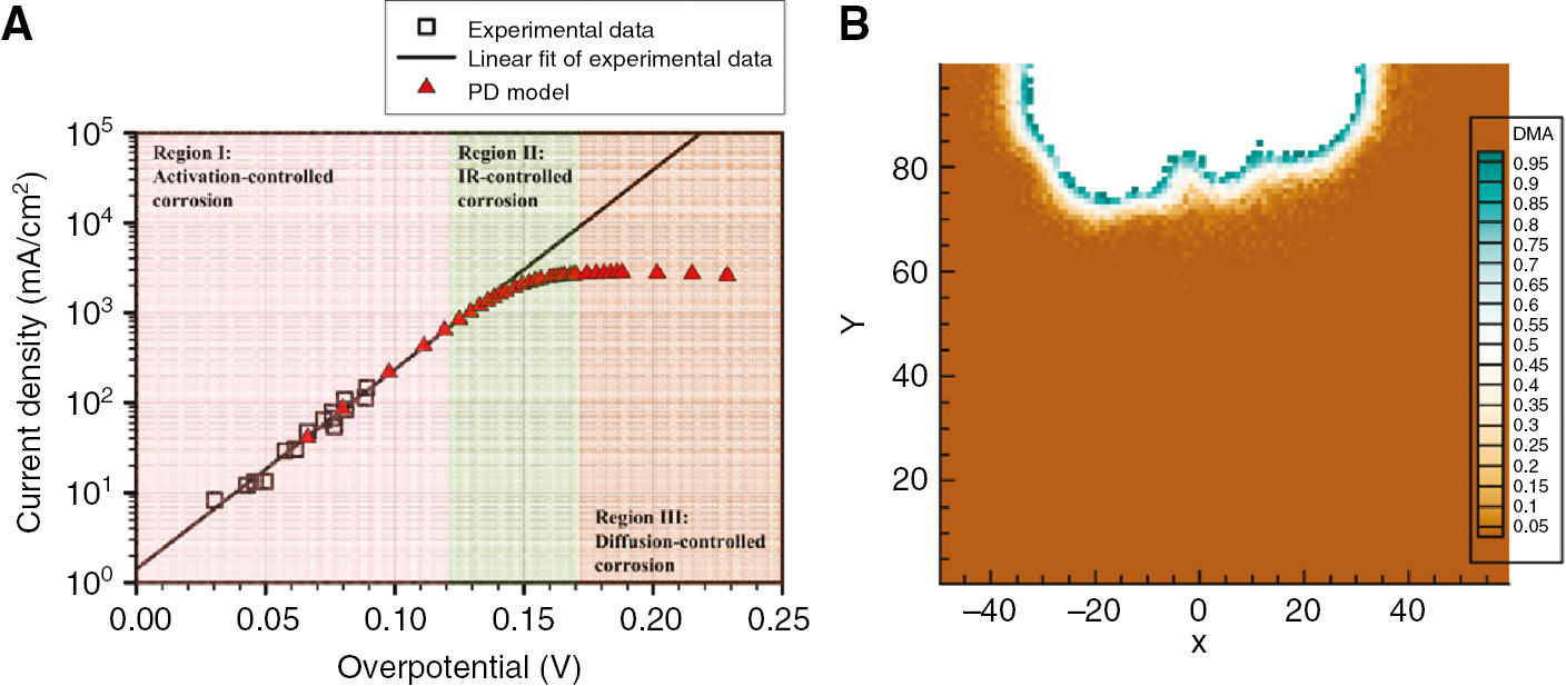
Peridynamic simulation results for pitting corrosion (Chen and Bobaru, 2015): (A) comparing current density versus overpotential from 1D peridynamic simulation results, with the experimental data on 1D artificial pitting in 304 stainless steel in 1 m NaCl solution (Gaudet et al., 1986); (B) a 2D peridynamic simulation of pit growth in a heterogeneous material. The colors in B map represent the damage values.
The mathematical formulation for the PD corrosion-damage model is given below, in a slightly modified version compared with the original formulation (Jafarzadeh et al., 2018a, 2019a,c):
Equation (9) is the PD diffusion equation as the nonlocal alternative to Eq. (7), the classical diffusion equation. For simplicity, in Eq. (9), C and
Schematics of different phases and different diffusion bonds at the corrosion front, in peridynamic corrosion damage model.
By selecting an appropriate relationship for kdiss, PD corrosion model can be easily modified to simulate any type of corrosion, including pitting corrosion, intergranular corrosion, etc. More generally, any chemo-physical behavior in the dissolution process can be captured by defining kdiss as a function of concentration of species, potential, current, temperature, material type, etc. For instance, a particular concentration-dependent relationship for kdiss is employed in Chen et al. (2016) and Jafarzadeh et al. (2018b) to address diffusion-controlled dissolution. Using a relationship based on the passivation criteria introduced in the LW model (see Section 3.1), the PD corrosion damage model is also capable of simulating the autonomous formation of lacy covers in pitting corrosion of stainless steel (Jafarzadeh et al., 2018b, 2019a). To model intergranular corrosion with a PD formulation, one can use different kdiss values for grains and grain boundaries, according to the mixed potential theory (Jafarzadeh et al., 2018a).
The autonomous propagation of the corrosion front is the result of Eq. (11) where the damage value (representing phases) changes with the molar concentration value of the metal atoms. According to this equation, C≤Csat is considered as the liquid phase, C=Csolid as intact solid, and the Csat<C<Csolid as the dissolving solid (see Figure 11). In the PD corrosion model, the dissolving solid region with 0<d<1 is noticed in the results shown in Figure 10B, and it corresponds to the DCL mentioned earlier.
In the PD corrosion damage model, the concentration-dependent damage evaluated from Eq. (11) is set to be the same with the mechanical damage resulting from elimination of mechanical bonds in PD fracture mechanics. A stochastic procedure is introduced in Chen and Bobaru (2015) to randomly eliminate the corresponding number of bonds for each node according to the damage value of that node [see Eq. (11)]. While the model’s equations are deterministic, this stochastic procedure for creating damage leads to pit shapes that are not perfectly symmetric, similar to real pits. Nevertheless, the differences between results obtained with different runs of the model are small, generally limited to the level of the horizon size, while the overall behavior is the same (Jafarzadeh et al., 2018b, 2019c).
Various numerical methods may be used to solve the PD corrosion-damage equation. The method that can also easily model the growth of cracks from corrosion pits in a combined mechano-chemical PD simulation is the meshfree discretization generated by a one-point Gaussian integration for the numerical quadrature of the integral in Eq. (9). For temporal integration, the forward-Euler method has been used to approximate the time derivative of C and update its value (Chen and Bobaru, 2015; Jafarzadeh et al., 2018a). Following the original formulation of the PD corrosion model, trusses-based FEM has also been used to implement the PD corrosion model in ANSYS software (De Meo and Oterkus, 2017).
Figures 12 and 13 show PD 2D and 3D simulation results next to their corresponding experiments.
![Figure 12:
Examples of 2D peridynamic simulations of localized corrosion: (A) experimental [left, from Ghahari et al. (2015)] and PD results for pitting corrosion in stainless steel, with formation of lacy covers; (B) experimental [left, from Zhang and Frankel (2002)] and PD simulation results for intergranular corrosion of AA2024 alloy at high potential from Jafarzadeh et al. (2018a). Colors in the computed results are the molar concentration of metal ions.](/document/doi/10.1515/corrrev-2019-0049/asset/graphic/j_corrrev-2019-0049_fig_040.jpg)
Examples of 2D peridynamic simulations of localized corrosion: (A) experimental [left, from Ghahari et al. (2015)] and PD results for pitting corrosion in stainless steel, with formation of lacy covers; (B) experimental [left, from Zhang and Frankel (2002)] and PD simulation results for intergranular corrosion of AA2024 alloy at high potential from Jafarzadeh et al. (2018a). Colors in the computed results are the molar concentration of metal ions.
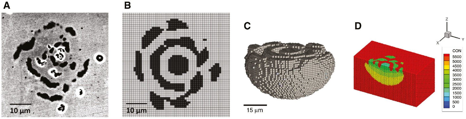
Comparison between experiments and 3D peridynamic simulation for pitting corrosion in stainless steel, with the formation of lacy covers (Jafarzadeh et al., 2019a): (A) the experimentally observed lacy cover morphology (Zakeri et al., 2015); (B) the lacy cover obtained in the PD simulation; (C) the 3D volume carved by the pit; (D) molar concentration map for the dissolved ions in a mid-cross-sectional view.
Compared with the non-autonomous models or the FVM and CA models discussed above, the PD model for corrosion damage has some advantages: (1) the propagation of the corrosion front is autonomous and does not depend on the discretization (in CA the particular discretization “drives” the model); (2) the model can incorporate any particular type of corrosion by specifying the kinetics via defining an appropriate kdiss in Eq. (10); (3) the use of two sets of bonds (mechanical, for monitoring damage, and diffusion bonds) allows natural extension to coupled chemo-mechanical models that can address stress-dependent corrosion and stress corrosion cracking (De Meo et al., 2017a,b; Chen et al., 2018; Li et al., 2018; Jafarzadeh et al., 2019b); and (4) the interface between the electrolyte and the corroding metal (the DCL) is naturally represented in this model as a layer in which mechanical and diffusion properties gradually change, much like how things are observed to happen in real corrosion of different alloy systems.
One of the drawbacks of the PD model for corrosion is the relatively high cost of computations, especially in 3D, due to nonlocality, which requires calculation of a volume integral at each node [see Eq. (9)]. Parallel and/or graphics processing unit-based computing are ways to speed up computations. A parallel implementation of PD models for fracture exists in Peridigm (Parks et al., 2012), an open-source code. Another issue in PD formulations is the treatment of “boundary” conditions and free surfaces. In a PD model, near the domain boundaries, the behavior is slightly different than in the bulk, due to the incomplete region of nonlocality. This is sometimes called “the PD surface effect”, and ways to resolve/minimize it are reviewed in Le and Bobaru (2018). Application of boundary conditions in the nonlocal settings is also different compared with the classical, local boundary conditions. Methods to apply nonlocal boundary conditions in ways equivalent to the local ones are described in Aksoylu et al. (2018).
3.2.4 PF models
PF modeling, also called “diffuse interface” modeling, has been used many years to model the evolution of interfaces between phases in a variety of problems, including solidification (Karma and Rappel, 1996), micro-structural evolution (Chen, 2002), phase transitions in ferroelectric (Chen, 2008) and ferromagnetic (Wang and Zhang, 2013) materials, etc. PF models have been recently adopted for simulating corrosion by modeling the evolution of the metal-electrolyte interface (Mai et al., 2016). Similar to PD model, in PF formulations the motion of the pit boundary is autonomous and part of the solution to the governing equations.
The PF corrosion model introduced by (Mai et al., 2016) is briefly reviewed here. In a two-phase domain, the PF φ(x, t) takes a value of 1 in one phase and 0 in the other phase. In PF, the interface between phases has a certain thickness (l), which introduces a length scale in the model. Over the interface region, φ is assigned a value between 0 and 1. A “free energy functional” for the system is defined: ℱ(φ, C) where C is the molar concentration of dissolved metal ions. The PF model for corrosion is a coupled system of PDEs for the evolution of the functions φ and C, such that ℱ is minimized:
Equation (12) is referred to as the Allen-Cahn equation and describes the phase transition. In this equation,
Equation (13) is a version of Cahn-Hilliard equation which expresses the evolution of the molar concentration of metal atoms. In this equation,
Other PF corrosion models (Ansari et al., 2018; Chadwick et al., 2018; Nguyen et al., 2018; Tsuyuki et al., 2018) are similar but may vary in some of the details from the one presented above. So far, PF corrosion models have been developed to simulate pitting corrosion (Mai et al., 2016; Ansari et al., 2018; Chadwick et al., 2018; Tsuyuki et al., 2018), galvanic corrosion (Mai and Soghrati, 2018), and stress-dependent corrosion (Mai and Soghrati, 2017; Ansari et al., 2018; Nguyen et al., 2018), mostly in 2D and recently in 3D (Tsuyuki et al., 2018; Lin et al., 2019).
Figure 14 shows two examples of PF simulations of pitting corrosion.
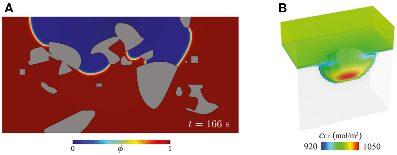
Examples for pitting corrosion simulations with phase-field models: (A) 2D simulation for a pit growing in a SiC particle-enforced aluminum composite (Mai et al., 2016). (B) 3D simulation of pitting corrosion in pure iron under a passive film (Tsuyuki et al., 2018). Colors in B map the molar concentration for Cl−.
Similar to PD corrosion models, the autonomous moving interface makes the PF formulation a flexible framework for predictive simulations of various types of corrosion. In PF models, phase-change and mass transfer processes are represented by two distinct but coupled PDEs: Equations (12) and (13). Such formulation adds a significant computational burden and algorithmic complexity in PF simulations (Soghrati et al., 2018). Note that PF models, while they introduce a length scale in the model via the thickness of the diffuse layer (PF transition zone between phases is an input in the problem), they are still local models with classical boundary conditions imposed on the set of PDEs.
Similar to subsurface partial damage in PD models, the diffuse interface in PF models leads to a transition region at the corrosion front. However, in a potential future PF-based model that includes damage, this layer has a pre-imposed structure (determined by the particular form selected for the free-energy functional), whereas in the PD models described above it is obtained as part of problem solution and depends on the nearby conditions around a point. This issue could be responsible for why PF models have failed in capturing the observed oscillatory behavior in thermally driven cracks that grow in thin glass plates, while PD models predict such behavior in great detail (Xu et al., 2018). Damage evolution in PF models depends strongly on the particular selection for the energy functional (Borden et al., 2012, 2016; Geelen et al., 2018).
4 Summary and discussion
In this section, we compare the reviewed models and summarize their advantages and disadvantages.
One class of the reviewed models is the non-autonomous type (Section 3.1), where one solves a version of Nernst-Plank equation for transport of ions inside the pit with a numerical method (e.g. FEM) and employs an additional technique to address the growth of the pit, such as updating the domain and remeshing the updated geometry or using level set method in a pre-discretized bi-phase domain.
In the other category, referred to as autonomous models, pit growth is directly addressed by phase evolution in the main formulation, together with the reaction and transport kinetics. As a major advantage, such approaches lead to autonomous pit growth without any additional effort. Computer implementation of these models is simplified because boundary tracking is no longer needed.
The four methods covered in more detail, and presented in Section 3.2, are of the “autonomous” type.
The finite volume model (Section 3.2.1) uses the FVM to solve the classical diffusion equation for mass transfer in the liquid and enforces a jump condition (based on mass conservation) to address dissolution and phase change in a multiphase domain.
CA (Section 3.2.2) employs state transition rules in a domain with discrete cells for transport, dissolution, and pit growth. The transition rules for dissolution are inspired by chemical reactions at the molecular level. CA is able to produce diverse pit morphologies similar to natural ones. However, time and spatial dimensions in CA are not physical quantities but rather model parameters. As such, they need to be calibrated to experimental measurements. Consequently, with this method, it is difficult to provide quantitative predictions of experimentally observed pit growth.
PD (Section 3.2.3) is a nonlocal model, which addresses the reaction kinetics, the transport kinetics, and the phase change for autonomous pit growth in one IDE using phase-dependent model parameters. This model employs the concept of mechanical damage to address the corroded region. As a result, it can be easily coupled with PD fracture models to better understand the dramatic loss of ductility and failure in materials exposed to corrosive environments and mechanical loading. This model has been shown to be predictive of a variety of experimental results and easily applicable to various types of corrosion via minimal modifications of model parameters. Nonlocality provides critical advantages in modeling damage in the layer affected by corrosion but also leads to relatively more expensive models to compute and may need specific treatment at the domain boundaries.
PF models (Section 3.2.4) solve a coupled system of PDEs for concentration of ions and phase evolution in the system, using the FEM or FDM, for example. Similar to PD, PF models are also flexible and predictive and can be utilized to simulate various types of corrosion in different materials. The coupled set of PDEs in the formulation of PF are, however, expensive to compute.
Table 1 compares the models reviewed in this study in terms of governing equations, boundary conditions, model strategies for pit growth, and computational cost.
Comparison of computational models for pitting corrosion.
| Non-autonomous (Section 3.1) | Finite volume model (Section 3.2.1) | Cellular automata (Section 3.2.2) | Peridynamic (Section 3.2.3) | Phase field (Section 3.2.4) | |
|---|---|---|---|---|---|
| Transport model | Classical transport equation (Nernst-Plank) | Classical diffusion equation | Transition rules for states of cells in a discrete domain | Peridynamic nonlocal diffusion equation | Cahn-Hilliard equation |
| Numerical method employed | Mostly FEM | FVM | Algorithms based on transition rules | Meshfree discretization with one-point Gaussian quadrature; FEM | FEM; FDM |
| Corrosion front | Boundary of a domain (requires boundary condition) | One layer of cells at the interface between the solid and the liquid subdomains | The interface between the solid cells and the liquid cells | The interface region between the solid and the liquid subdomains | A thick diffuse interface between solid and liquid phases |
| Dissolution flux | Found from applied boundary condition | Imposed jump condition and mass conservation | Rate of state change of solid cells to liquid cells | Nonlocal diffusion flux, defined over the interface | A flux through the diffuse interface |
| Pit growth | Moving boundary according to Stefan-type condition | Autonomous growth via phase change according to concentration values | Autonomous growth via transition rules for solid cells | Autonomous growth via phase change induced by concentration-dependent damage | Phase change via Allen-Cahn equation |
| Advantages | Well-established framework and commercialized | Autonomous pit growth | Autonomous pit growth; chemical details can be included; complex realistically looking pit morphologies | Autonomous pit growth; easy to modify; captures mechanical damage and DCL; micro-randomness; predictive pit morphologies, lacy-covers | Autonomous pit growth; flexible model |
| Disadvantages | Boundary tracking and domain updating is required (complex and costly) | Does not capture mechanical damage and DCL; discretization dependency | Difficult to calibrate; grid size and time not physical parameters; discretization dependency | Nonlocal effects at boundaries; computational cost | Computational cost; dense mathematical framework (coupled PDEs) |
5 Prospects
In this section we discuss some of the open areas for future research in corrosion modeling.
5.1 Multi-field universal models
As mentioned in Section 1, corrosion is a complex and highly interdisciplinary phenomenon. Evolution of the dissolution-induced damage can depend on a variety of factors, such as the electric potential field, temperature field, stress field, pH field, corrosion product formation, etc. Most of the existing models include only one or two of these factors. Such simplifications make the models applicable only to limited cases. A more general multi-field model will be able to address all corrosion types: pitting, galvanic, stress-assisted, stress corrosion cracking, and the various mechano-chemical environments within a unified framework.
5.2 Multi-scale models
Corrosion-induced failure is a multi-scale phenomenon: it depends on chemical reactions at the molecular level (nano-scale), on the microstructure of the alloy (microscale), and on the environment and loading conditions applied to the structure (macro-scale). Nanoscale processes can currently be modeled by molecular dynamics, microscale processes can be simulated with one of the reviewed models, while macroscale effects can be captured using continuum and probabilistic models. A multiscale corrosion damage model that bridges the nano, micro, and macro scales would be very useful.
5.3 Utilizing artificial intelligence and big data
The recent steps in machine learning and processing of big data opens new avenues for utilizing these tools in extending the reach of corrosion modeling. It would be interesting to find how one can incorporate artificial intelligence and big data into existing mechanistic corrosion models in order to improve predictability, reliability, and universality of corrosion models. There are also steps taken to create “model-free” artificial intelligence systems that try to predict physical behavior from measurement data alone. Whether such approaches can be applied to predicting the complex corrosion-induced damage and fracture remains an open question.
5.4 Experiments
Computational models indeed can benefit from high-resolution 4D characterization of corrosion damage using advanced material characterization methods. Based on experimental observations, one can deepen the understanding of the corrosion mechanism and update existing corrosion models accordingly.
5.5 Numerical methods
Any new numerical method that reduces the computational cost for corrosion models can make a large impact. Such methods, when applied to, for example, the relatively expensive PD and PF models, can allow simulation of corrosion damage over larger domains and time spans.
5.6 Design
Once progress in any of the areas mentioned above takes place, one can then develop optimal material design strategies that account for corrosion damage and fracture in the life of the structure/system. This will also have an effect on the best practices for corrosion prevention methods.
6 Conclusions
This paper presented a review of computational modeling for pitting corrosion, including the most recent advances and approaches. Most of the computational pitting corrosion models use anodic dissolution and transport kinetics in the electrolyte as the basis for their governing equations. Here, we classified these models into two categories, depending on how the propagation of the corrosion front is computed: non-autonomous models (which require updating and tracking of the corrosion front) and autonomous models (in which the evolution of the corrosion front is part of the main formulation).
Non-autonomous models are based on solving the classical transport equation (simplified versions of Nernst-Planck equation) with a numerical method (e.g. FEM) to compute the transport kinetics in the electrolyte. Tracking pit growth is addressed as a separate part and adds significant complexity. In contrast, autonomous models obtain the motion of the corrosion front directly as part of the solution of the main formulation. The autonomous models reviewed here were the following: a finite volume approach, the CA techniques, the PD model for corrosion damage, and PF models.
We compared the reviewed models with each other and discussed their relative advantages and disadvantages. Some open research areas for further development in corrosion modeling were also noted.
Funding source: National Natural Science Foundation of China
Award Identifier / Grant number: 11802098
Award Identifier / Grant number: D1418010
Funding statement: This work has been supported by the ONR project “SCC: the Importance of Damage Evolution in the Layer Affected by Corrosion” (program manager William Nickerson) and by the AFOSR, Funder Id: http://dx.doi.org/10.13039/100000181, MURI Center for Materials Failure Prediction through Peridynamics (program managers Jaimie Tiley, David Stargel, Ali Sayir, Fariba Fahroo, and James Fillerup). Z.C. was supported by the National Natural Science Foundation of China (Funder Id: http://dx.doi.org/10.13039/501100001809, 11802098 and D1418010).
About the authors

Siavash Jafarzadeh received his BSc (2011) and MSc (2015) degrees in Mechanical Engineering from Isfahan University of Technology, Isfahan, Iran. In 2016, he started his PhD program in Mechanical Engineering and Applied Mechanics at University of Nebraska-Lincoln, USA. His doctoral research is focused on computational modeling of corrosion damage and stress corrosion cracking, using peridynamic theory.

Ziguang Chen received his PhD degree in Mechanical Engineering and Applied Mechanics from University of Nebraska-Lincoln, USA, in 2012. He worked as a postdoctoral researcher in the same university from 2013 to 2017. He is currently a Professor in the Department of Mechanics at Huazhong University of Science and Technology, China.

Florin Bobaru received his BS (1995) and MS (1997) degrees in Mathematics and Mechanics from University of Bucharest, Romania, and his PhD (2001) degree in Theoretical and Applied Mechanics from Cornell University, USA. He is currently a Professor and Hergenrader Distinguished Scholar in Mechanical and Materials Engineering at University of Nebraska-Lincoln, USA. He is the main editor of the Handbook of Peridynamic Modeling (2017).
References
Aksoylu B, Celiker F, Kilicer O. Nonlocal operators with local boundary conditions: an overview. In: Voyiadjis G, editor. Handbook of nonlocal continuum mechanics for materials and structures. Springer, 2018: 1–38.10.1007/978-3-319-22977-5_34-1Search in Google Scholar
Amaya K, Yoneya N, Onishi Y. Obtaining corrosion rates by bayesian estimation: numerical simulation coupled with data. Electrochem Soc Interface 2014; 23: 53–57.10.1149/2.F03144IFSearch in Google Scholar
Ansari TQ, Xiao Z, Hu S, Li Y, Luo J-L, Shi S-Q. Phase-field model of pitting corrosion kinetics in metallic materials. npj Comp Mater 2018; 4: 38.10.1038/s41524-018-0089-4Search in Google Scholar
Badwe N, Chen X, Schreiber D, Olszta M, Overman N, Karasz E, Tse A, Bruemmer S, Sieradzki K. Decoupling the role of stress and corrosion in the intergranular cracking of noble-metal alloys. Nat Mater 2018; 17: 887–893.10.1038/s41563-018-0162-xSearch in Google Scholar PubMed
Bard AJ, Faulkner LR, Leddy J, Zoski CG. Electrochemical methods: fundamentals and applications. New York: Wiley, 1980.Search in Google Scholar
Bažant ZP. Why continuum damage is nonlocal: micromechanics arguments. J Eng Mech 1991; 117: 1070–1087.10.1061/(ASCE)0733-9399(1991)117:5(1070)Search in Google Scholar
Bažant ZP, Jirásek M. Nonlocal integral formulations of plasticity and damage: survey of progress. J Eng Mech 2002; 128: 1119–1149.10.1061/(ASCE)0733-9399(2002)128:11(1119)Search in Google Scholar
Behzadinasab M, Vogler TJ, Peterson AM, Rahman R, Foster JT. Peridynamics modeling of a shock wave perturbation decay experiment in granular materials with intra-granular fracture. J Dyn Behav Mater 2018; 4: 529–542.10.1007/s40870-018-0174-2Search in Google Scholar
Bhandari J, Khan F, Abbassi R, Garaniya V, Ojeda R. Modelling of pitting corrosion in marine and offshore steel structures – a technical review. J Loss Prev Process Ind 2015; 37: 39–62.10.1016/j.jlp.2015.06.008Search in Google Scholar
Bobaru F, Duangpanya M. The peridynamic formulation for transient heat conduction. Int J Heat Mass Transfer 2010; 53: 4047–4059.10.1016/j.ijheatmasstransfer.2010.05.024Search in Google Scholar
Bobaru F, Duangpanya M. A peridynamic formulation for transient heat conduction in bodies with evolving discontinuities. J Comput Phys 2012; 231: 2764–2785.10.1016/j.jcp.2011.12.017Search in Google Scholar
Bobaru F, Zhang G. Why do cracks branch? A peridynamic investigation of dynamic brittle fracture. Int J Fracture 2015; 196: 59–98.10.1007/s10704-015-0056-8Search in Google Scholar
Bobaru F, Foster JT, Geubelle PH, Silling SA, editors. Handbook of peridynamic modeling. Boca Raton, FL, USA: CRC Press/Taylor and Francis, 2017.10.1201/9781315373331Search in Google Scholar
Bobaru F, Mehrmashhadi J, Chen Z, Niazi S. Intraply fracture in fiber-reinforced composites: a peridynamic analysis. ASC 33rd Annual Technical Conference & 18th US-Japan Conference on Composite Materials, Seattle. 2018: 1–9.10.12783/asc33/26039Search in Google Scholar
Borden MJ, Verhoosel CV, Scott MA, Hughes TJ, Landis CM. A phase-field description of dynamic brittle fracture. Comput Meth Appl Mech Eng 2012; 217: 77–95.10.1016/j.cma.2012.01.008Search in Google Scholar
Borden MJ, Hughes TJ, Landis CM, Anvari A, Lee IJ. A phase-field formulation for fracture in ductile materials: finite deformation balance law derivation, plastic degradation, and stress triaxiality effects. Comput Meth Appl Mech Eng 2016; 312: 130–166.10.1016/j.cma.2016.09.005Search in Google Scholar
Cattant F, Crusset D, Féron D. Corrosion issues in nuclear industry today. Mater Today 2008; 11: 32–37.10.1016/S1369-7021(08)70205-0Search in Google Scholar
Chadwick AF, Stewart JA, Enrique RA, Du S, Thornton K. Numerical modeling of localized corrosion using phase-field and smoothed boundary methods. J Electrochem Soc 2018; 165: C633–C646.10.1149/2.0701810jesSearch in Google Scholar
Chen L-Q. Phase-field models for microstructure evolution. Annu Rev Mater Res 2002; 32: 113–140.10.1146/annurev.matsci.32.112001.132041Search in Google Scholar
Chen LQ. Phase-field method of phase transitions/domain structures in ferroelectric thin films: a review. J Am Ceram Soc 2008; 91: 1835–1844.10.1111/j.1551-2916.2008.02413.xSearch in Google Scholar
Chen S, Doolen GD. Lattice Boltzmann method for fluid flows. Annu Rev Fluid Mech 1998; 30: 329–364.10.1146/annurev.fluid.30.1.329Search in Google Scholar
Chen Z, Bobaru F. Peridynamic modeling of pitting corrosion damage. J Mech Phys Solids 2015; 78: 352–381.10.1016/j.jmps.2015.02.015Search in Google Scholar
Chen Y, Liou Y, Shih H. Stress corrosion cracking of type 321 stainless steels in simulated petrochemical process environments containing hydrogen sulfide and chloride. Mater Sci Eng A 2005; 407: 114–126.10.1016/j.msea.2005.07.011Search in Google Scholar
Chen Z, Zhang G, Bobaru F. The influence of passive film damage on pitting corrosion. J Electrochem Soc 2016; 163: C19–C24.10.1149/2.0521602jesSearch in Google Scholar
Chen Z, Jafarzadeh S, Li S, Bobaru F, Qian Q. Peridynamic mechano-chemical modeling of stress corrosion cracking. Proceedings IRF2018: 6th International Conference Integrity-Reliability-Failure. Lisbon, Portugal: INEGI/FEUP, 2018: 299–300.Search in Google Scholar
Chen Z, Niazi S, Zhang G, Bobaru F. Peridynamic functionally graded and porous materials: modeling fracture and damage. In: Voyiadjis GZ, editor. Handbook of Nonlocal Continuum Mechanics for Materials and Structures. Springer, 2019: 1353–1387, doi: https://doi.org/10.1007/978-3-319-58729-5_3610.1007/978-3-319-58729-5_36Search in Google Scholar
Chowdhury D, Santen L, Schadschneider A. Statistical physics of vehicular traffic and some related systems. Phys Rep 2000; 329: 199–329.10.1016/S0370-1573(99)00117-9Search in Google Scholar
Chuanjie C, Rujin M, Airong C, Zichao P, Hao T. Experimental study and 3D cellular automata simulation of corrosion pits on Q345 steel surface under salt-spray environment. Corros Sci 2019; 154: 80–89.10.1016/j.corsci.2019.03.011Search in Google Scholar
Co NEC, Burns JT. Effects of macro-scale corrosion damage feature on fatigue crack initiation and fatigue behavior. Int J Fatigue 2017; 103: 234–247.10.1016/j.ijfatigue.2017.05.028Search in Google Scholar
Cui J, Yang F, Yang T-H, Yang G-F. Numerical study of stainless steel pitting process based on the lattice Boltzmann method. Int J Electrochem Sci 2019; 14: 1529–1545.10.20964/2019.02.47Search in Google Scholar
De Meo D, Oterkus E. Finite element implementation of a peridynamic pitting corrosion damage model. Ocean Eng 2017; 135: 76–83.10.1016/j.oceaneng.2017.03.002Search in Google Scholar
De Meo D, Russo L, Oterkus E. Modeling of the onset, propagation, and interaction of multiple cracks generated from corrosion pits by using peridynamics. J Eng Mater Technol 2017a; 139: 041001.10.1115/1.4036443Search in Google Scholar
De Meo D, Russo L, Oterkus E, Gunasegaram D, Cole I. Peridynamics for predicting pit-to-crack transition. 58th AIAA/ASCE/AHS/ASC Structures, Structural Dynamics, and Materials Conference. 2017b: 0568, doi: https://doi.org/10.2514/6.2017-056810.2514/6.2017-0568Search in Google Scholar
Di Caprio D, Vautrin-Ul C, Stafiej J, Saunier J, Chaussé A, Féron D, Badiali J. Morphology of corroded surfaces: contribution of cellular automaton modelling. Corros Sci 2011; 53: 418–425.10.1016/j.corsci.2010.09.052Search in Google Scholar
Di Caprio D, Stafiej J, Luciano G, Arurault L. 3D cellular automata simulations of intra and intergranular corrosion. Corros Sci 2016; 112: 438–450.10.1016/j.corsci.2016.07.028Search in Google Scholar
Duddu R. Numerical modeling of corrosion pit propagation using the combined extended finite element and level set method. Comput Mech 2014; 54: 613–627.10.1007/s00466-014-1010-8Search in Google Scholar
Encinas AH, Encinas LH, White SH, del Rey AM, Sánchez GR. Simulation of forest fire fronts using cellular automata. Adv Eng Softw 2007; 38: 372–378.10.1016/j.advengsoft.2006.09.002Search in Google Scholar
Ernst P, Newman R. Pit growth studies in stainless steel foils. II. Effect of temperature, chloride concentration and sulphate addition. Corros Sci 2002; 44: 943–954.10.1016/S0010-938X(01)00134-2Search in Google Scholar
Frankel G. Pitting corrosion of metals a review of the critical factors. J Electrochem Soc 1998; 145: 2186–2198.10.1149/1.1838615Search in Google Scholar
Gaudet G, Mo W, Hatton T, Tester J, Tilly J, Isaacs HS, Newman R. Mass transfer and electrochemical kinetic interactions in localized pitting corrosion. AlChE J 1986; 32: 949–958.10.1002/aic.690320605Search in Google Scholar
Geelen RJ, Liu Y, Hu T, Tupek MR, Dolbow JE. A phase-field formulation for dynamic cohesive fracture. Comput Methods Appl Mech Eng 2019; 348: 680–711.10.1016/j.cma.2019.01.026Search in Google Scholar
Ghahari SM. In situ synchrotron X-ray characterisation and modelling of pitting corrosion of stainless steel. PhD thesis, University of Birmingham, 2012.Search in Google Scholar
Ghahari S, Krouse D, Laycock N, Rayment T, Padovani C, Suter T, Mokso R, Marone F, Stampanoni M, Monir M. Pitting corrosion of stainless steel: measuring and modelling pit propagation in support of damage prediction for radioactive waste containers. Corros Eng Sci Techn 2011; 46: 205–211.10.1179/1743278211Y.0000000003Search in Google Scholar
Ghahari M, Krouse D, Laycock N, Rayment T, Padovani C, Stampanoni M, Marone F, Mokso R, Davenport AJ. Synchrotron X-ray radiography studies of pitting corrosion of stainless steel: extraction of pit propagation parameters. Corros Sci 2015; 100: 23–35.10.1016/j.corsci.2015.06.023Search in Google Scholar
Ha YD, Bobaru F. Studies of dynamic crack propagation and crack branching with peridynamics. Int J Fracture 2010; 162: 229–244.10.1007/978-90-481-9760-6_18Search in Google Scholar
Horner D, Connolly B, Zhou S, Crocker L, Turnbull A. Novel images of the evolution of stress corrosion cracks from corrosion pits. Corros Sci 2011; 53: 3466–3485.10.1016/j.corsci.2011.05.050Search in Google Scholar
Huang Y, Tu S-T, Xuan F-Z. Pit to crack transition behavior in proportional and non-proportional multiaxial corrosion fatigue of 304 stainless steel. Eng Fract Mech 2017; 184: 259–272.10.1016/j.engfracmech.2017.08.019Search in Google Scholar
Isaacs H, Cho JH, Rivers M, Sutton S. In situ X-ray microprobe study of salt layers during anodic dissolution of stainless steel in chloride solution. J Electrochem Soc 1995; 142: 1111–1118.10.1149/1.2044138Search in Google Scholar
Jafarzadeh S, Chen Z, Bobaru F. Peridynamic modeling of intergranular corrosion damage. J Electrochem Soc 2018a; 165: C362–C374.10.1149/2.0821807jesSearch in Google Scholar
Jafarzadeh S, Chen Z, Bobaru F. Peridynamic modeling of repassivation in pitting corrosion of stainless steel. Corrosion 2018b; 74: 393–414.10.5006/2615Search in Google Scholar
Jafarzadeh S, Chen Z, Bobaru F. Predictive peridynamic 3D models of pitting corrosion in stainless steel with formation of lacy covers. CORROSION 2019. NACE International, 2019a: paper no. 13374.10.5006/C2019-13374Search in Google Scholar
Jafarzadeh S, Chen Z, Zhao J, Bobaru F. 3D peridynamic models for pitting corrosion and stress corrosion cracking. Meeting abstracts. The Electrochemical Society, 2019b: No. 999.10.1149/MA2019-01/16/999Search in Google Scholar
Jafarzadeh S, Chen Z, Zhao J, Bobaru F. Pitting, lacy covers, and pit merger in stainless steel: 3D peridynamic models. Corros Sci 2019c; 150: 17–31.10.1016/j.corsci.2019.01.006Search in Google Scholar
Jones DA. Principles and prevention of corrosion. Macmillan, 1992.Search in Google Scholar
Jones DA. Principles and prevention of corrosion, 2nd ed. Upper Saddle River, NY: Prentice Hall, 1996.Search in Google Scholar
Karma A, Rappel W-J. Phase-field method for computationally efficient modeling of solidification with arbitrary interface kinetics. Phys Rev E 1996; 53: R3017.10.1103/PhysRevE.53.R3017Search in Google Scholar PubMed
Krouse D, Laycock N, Padovani C. Modelling pitting corrosion of stainless steel in atmospheric exposures to chloride containing environments. Corros Eng Sci Techn 2014; 49: 521–528.10.1179/1743278214Y.0000000221Search in Google Scholar
Laycock N, White S. Computer simulation of single pit propagation in stainless steel under potentiostatic control. J Electrochem Soc 2001; 148: B264–B275.10.1149/1.1376119Search in Google Scholar
Laycock N, White S, Noh J, Wilson P, Newman R. Perforated covers for propagating pits. J Electrochem Soc 1998; 145: 1101–1108.10.1149/1.1838423Search in Google Scholar
Laycock NJ, Krouse DP, Hendy SC, Williams DE. Computer simulation of pitting corrosion of stainless steels. Electrochem Soc Interface 2014; 23: 65–71.10.1149/2.F05144IFSearch in Google Scholar
Le Q, Bobaru F. Surface corrections for peridynamic models in elasticity and fracture. Comput Mech 2018; 61: 499–518.10.1007/s00466-017-1469-1Search in Google Scholar
Lee Y, Kouvroukoglou S, McIntire LV, Zygourakis K. A cellular automaton model for the proliferation of migrating contact-inhibited cells. Biophys J 1995; 69: 1284–1298.10.1016/S0006-3495(95)79996-9Search in Google Scholar PubMed PubMed Central
Li S, Xu Y, Li H, Guan X. Uniform and pitting corrosion modeling for high-strength bridge wires. J Bridge Eng 2014; 19: 04014025.10.1061/(ASCE)BE.1943-5592.0000598Search in Google Scholar
Li S, Chen Z, Wang F, Cui B, Tan L, Bobaru F. Analysis of corrosion-induced diffusion layer in ZK60A magnesium alloy. J Electrochem Soc 2016; 163: C784–C790.10.1149/2.1001613jesSearch in Google Scholar
Li S, Chen Z, Tan L, Bobaru F. Corrosion-induced embrittlement in ZK60A Mg alloy. Mater Sci Eng A 2018; 713: 7–17.10.1016/j.msea.2017.12.053Search in Google Scholar
Lin C, Ruan H, Shi S-Q. Phase field study of mechanico-electrochemical corrosion. Electrochim Acta 2019; 310: 240–255.10.1016/j.electacta.2019.04.076Search in Google Scholar
Liu C, Kelly R. The use of finite element methods (FEM) in the modeling of localized corrosion. Electrochem Soc Interface 2014; 23: 47–51.10.1149/2.F02144IFSearch in Google Scholar
Liu M, Qiu D, Zhao M-C, Song G, Atrens A. The effect of crystallographic orientation on the active corrosion of pure magnesium. Scripta Mater 2008a; 58: 421–424.10.1016/j.scriptamat.2007.10.027Search in Google Scholar
Liu Z, Li X, Du C, Zhai G, Cheng Y. Stress corrosion cracking behavior of X70 pipe steel in an acidic soil environment. Corros Sci 2008b; 50: 2251–2257.10.1016/j.corsci.2008.05.011Search in Google Scholar
Liu R, Li T, Liu L, Cui Y, Oguzie EE, Li Y, Wang F. Cellular automata study of the combined effects of passive film breakdown and repassivation on metastable pits on sputtered nanocrystalline stainless steel. J Electrochem Soc 2019; 166: C91–C100.10.1149/2.0921904jesSearch in Google Scholar
Mai W, Soghrati S. A phase field model for simulating the stress corrosion cracking initiated from pits. Corros Sci 2017; 125: 87–98.10.1016/j.corsci.2017.06.006Search in Google Scholar
Mai W, Soghrati S. New phase field model for simulating galvanic and pitting corrosion processes. Electrochim Acta 2018; 260: 290–304.10.1016/j.electacta.2017.12.086Search in Google Scholar
Mai W, Soghrati S, Buchheit RG. A phase field model for simulating the pitting corrosion. Corros Sci 2016; 110: 157–166.10.1016/j.corsci.2016.04.001Search in Google Scholar
Malki B, Baroux B. Computer simulation of the corrosion pit growth. Corros Sci 2005; 47: 171–182.10.1016/j.corsci.2004.05.004Search in Google Scholar
Marcus P. Corrosion mechanisms in theory and practice. Boca Raton, FL, USA: CRC Press, 2011.Search in Google Scholar
Marcus P, Maurice V. Atomic level characterization in corrosion studies. Philos Trans A Math Phys Eng Sci 2017; 375: 20160414.10.1098/rsta.2016.0414Search in Google Scholar PubMed
Marzban B. A multiphysics computational framework for understanding cell and microtissue morphogenesis. PhD thesis, University of Rhode Island, 2018.Search in Google Scholar
Mehrmashhadi J, Tang Y, Zhao X, Xu Z, Pan JJ, Van Le Q, BobaruF. The effect of solder joint microstructure on the drop test failure – a peridynamic analysis. IEEE Trans Compon Packaging Manuf Technol 2019; 9: 58–71.10.1109/TCPMT.2018.2862898Search in Google Scholar
National Transportation Safety Board. Collapse of I-35W highway bridge, Minneapolis, Minnesota, August 1, 2007, Washington, DC, 2008.Search in Google Scholar
Nguyen TT, Bolivar J, Shi Y, Réthoré J, King A, Fregonese M, Adrien J, Buffiere J, Baietto M. A phase field method for modeling anodic dissolution induced stress corrosion crack propagation. Corros Sci 2018; 132: 146–160.10.1016/j.corsci.2017.12.027Search in Google Scholar
Oterkus S, Madenci E, Agwai A. Peridynamic thermal diffusion. J Comput Phys 2014; 265: 71–96.10.1016/j.jcp.2014.01.027Search in Google Scholar
Pantelakis SG, Daglaras P, Apostolopoulos CA. Tensile and energy density properties of 2024, 6013, 8090 and 2091 aircraft aluminum alloy after corrosion exposure. Theor Appl Fract Mec 2000; 33: 117–134.10.1016/S0167-8442(00)00007-0Search in Google Scholar
Parks ML, Littlewood DJ, Mitchell JA, Silling SA. Peridigm users’ guide v1. 0.0. Sand Rep 2012: 7800.10.2172/1055619Search in Google Scholar
Pérez-Brokate CF, di Caprio D, Féron D, de Lamare J, Chaussé A. Three dimensional discrete stochastic model of occluded corrosion cell. Corros Sci 2016; 111: 230–241.10.1016/j.corsci.2016.04.009Search in Google Scholar
Pidaparti RM, Fang L, Palakal MJ. Computational simulation of multi-pit corrosion process in materials. Comp Mater Sci 2008; 41: 255–265.10.1016/j.commatsci.2007.04.017Search in Google Scholar
Pistorius P, Burstein G. Metastable pitting corrosion of stainless steel and the transition to stability. Phil Trans R Soc Lond A 1992; 341: 531–559.10.1098/rsta.1992.0114Search in Google Scholar
Rahmati AR, Niazi S. Simulation of microflows using the lattice Boltzmann method on nonuniform meshes. Nanosci Technol 2012; 3: 77–97.10.1615/NanomechanicsSciTechnolIntJ.v3.i1.40Search in Google Scholar
Rahmati AR, Niazi S. Entropic lattice Boltzmann method for microflow simulation. Nanosci Technol 2014; 5: 153–167.10.1615/NanomechanicsSciTechnolIntJ.v5.i2.60Search in Google Scholar
Rahmati AR, Niazi S, Beni MN. Natural convection flow simulation of nanofluid in a square cavity using an incompressible generalized lattice Boltzmann method. Defect and diffusion forum. Trans Tech Publ 2012: 69–79.10.4028/www.scientific.net/DDF.329.69Search in Google Scholar
Rani S, Agrawal AK, Rastogi V. Failure analysis of a first stage IN738 gas turbine blade tip cracking in a thermal power plant. Case Studies in Engineering Failure Analysis 2017; 8: 1–10.10.1016/j.csefa.2016.11.002Search in Google Scholar
Revie RW. Corrosion and corrosion control: an introduction to corrosion science and engineering. John Wiley & Sons, 2008.10.1002/9780470277270Search in Google Scholar
Rusyn B, Tors’Ka R, Pokhmurs’kyi AY. Modeling of the evolution of corrosion pitting with the use of cellular automata. Mater Sci 2015; 50: 706–713.10.1007/s11003-015-9775-2Search in Google Scholar
Scheiner S, Hellmich C. Stable pitting corrosion of stainless steel as diffusion-controlled dissolution process with a sharp moving electrode boundary. Corros Sci 2007; 49: 319–346.10.1016/j.corsci.2006.03.019Search in Google Scholar
Scheiner S, Hellmich C. Finite volume model for diffusion-and activation-controlled pitting corrosion of stainless steel. Comput Methods Appl Mech Eng 2009; 198: 2898–2910.10.1016/j.cma.2009.04.012Search in Google Scholar
Shahryari A, Szpunar JA, Omanovic S. The influence of crystallographic orientation distribution on 316LVM stainless steel pitting behavior. Corros Sci 2009; 51: 677–682.10.1016/j.corsci.2008.12.019Search in Google Scholar
Sharland S. A mathematical model of crevice and pitting corrosion – II. The mathematical solution. Corros Sci 1988; 28: 621–630.10.1016/0010-938X(88)90028-5Search in Google Scholar
Sharland S, Tasker P. A mathematical model of crevice and pitting corrosion – I. The physical model. Corros Sci 1988; 28: 603–620.10.1016/0010-938X(88)90027-3Search in Google Scholar
Sharland S, Jackson C, Diver A. A finite-element model of the propagation of corrosion crevices and pits. Corros Sci 1989; 29: 1149–1166.10.1016/0010-938X(89)90051-6Search in Google Scholar
Sheng J, Xia J. Effect of simulated pitting corrosion on the tensile properties of steel. Const Build Mater 2017; 131: 90–100.10.1016/j.conbuildmat.2016.11.037Search in Google Scholar
Silling SA. Reformulation of elasticity theory for discontinuities and long-range forces. J Mech Phys Solids 2000; 48: 175–209.10.1016/S0022-5096(99)00029-0Search in Google Scholar
Silling SA, Lehoucq R. Peridynamic theory of solid mechanics. In: Aref H, Giessen Evd, editors. Advances in Appled Mechanics. Elsevier, 2010: 73–168.10.1016/S0065-2156(10)44002-8Search in Google Scholar
Soghrati S, Chen Y, Mai W. A non-iterative local remeshing approach for simulating moving boundary transient diffusion problems. Finite Elem Anal Des 2018; 140: 23–37.10.1016/j.finel.2017.11.001Search in Google Scholar
Song R, Blawert C, Dietzel W, Atrens A. A study on stress corrosion cracking and hydrogen embrittlement of AZ31 magnesium alloy. Mater Sci Eng A 2005; 399: 308–317.10.1016/j.msea.2005.04.003Search in Google Scholar
Stafiej J, di Caprio D, Bartosik Ł. Corrosion-passivation processes in a cellular automata based simulation study. J Supercomput 2013; 65: 697–709.10.1007/s11227-013-0933-8Search in Google Scholar
Taylor CD. Modeling corrosion, atom by atom. Electrochem Soc Interface 2014; 23: 59–64.10.1149/2.F04144IFSearch in Google Scholar
Taylor CD, Marcus P. Molecular modeling of corrosion processes: scientific development and engineering applications. John Wiley & Sons, 2015.10.1002/9781119057666Search in Google Scholar
Tian W, Du N, Li S, Chen S, Wu Q. Metastable pitting corrosion of 304 stainless steel in 3.5% NaCl solution. Corros Sci 2014; 85: 372–379.10.1016/j.corsci.2014.04.033Search in Google Scholar
Tsuyuki C, Yamanaka A, Ogimoto Y. Phase-field modeling for pH-dependent general and pitting corrosion of iron. Sci Rep 2018; 8: 12777.10.1038/s41598-018-31145-7Search in Google Scholar PubMed PubMed Central
Turnbull A, Wright L, Crocker L. New insight into the pit-to-crack transition from finite element analysis of the stress and strain distribution around a corrosion pit. Corros Sci 2010; 52: 1492–1498.10.1016/j.corsci.2009.12.004Search in Google Scholar
Vagbharathi A, Gopalakrishnan S. An extended finite-element model coupled with level set method for analysis of growth of corrosion pits in metallic structures. Proc R Soc A 2014; 470: 20140001.10.1098/rspa.2014.0001Search in Google Scholar
Vallabhaneni R, Stannard TJ, Kaira CS, Chawla N. 3D X-ray microtomography and mechanical characterization of corrosion-induced damage in 7075 aluminium (Al) alloys. Corros Sci 2018; 139: 97–113.10.1016/j.corsci.2018.04.046Search in Google Scholar
Valor A, Caleyo F, Alfonso L, Rivas D, Hallen J. Stochastic modeling of pitting corrosion: a new model for initiation and growth of multiple corrosion pits. Corros Sci 2007; 49: 559–579.10.1016/j.corsci.2006.05.049Search in Google Scholar
Van der Weeën P, Zimer AM, Pereira EC, Mascaro LH, Bruno OM, De Baets B. Modeling pitting corrosion by means of a 3D discrete stochastic model. Corros Sci 2014; 82: 133–144.10.1016/j.corsci.2014.01.010Search in Google Scholar
Velázquez J, Caleyo F, Valor A, Hallen J. Predictive model for pitting corrosion in buried oil and gas pipelines. Corrosion 2009; 65: 332–342.10.5006/1.3319138Search in Google Scholar
Verma C, Lgaz H, Verma D, Ebenso EE, Bahadur I, Quraishi M. Molecular dynamics and Monte Carlo simulations as powerful tools for study of interfacial adsorption behavior of corrosion inhibitors in aqueous phase: a review. J Mol Liq 2018; 260: 99–120.10.1016/j.molliq.2018.03.045Search in Google Scholar
Walton JC. Mathematical modeling of mass transport and chemical reaction in crevice and pitting corrosion. Corros Sci 1990; 30: 915–928.10.1016/0010-938X(90)90013-USearch in Google Scholar
Walton J, Cragnolino G, Kalandros S. A numerical model of crevice corrosion for passive and active metals. Corros Sci 1996; 38: 1–18.10.1016/0010-938X(96)00107-2Search in Google Scholar
Wang J, Zhang J. A real-space phase field model for the domain evolution of ferromagnetic materials. Int J Solids Struct 2013; 50: 3597–3609.10.1016/j.ijsolstr.2013.07.001Search in Google Scholar
Xiao J, Chaudhuri S. Predictive modeling of localized corrosion: an application to aluminum alloys. Electrochim Acta 2011; 56: 5630–5641.10.1016/j.electacta.2011.04.019Search in Google Scholar
Xu Z, Zhang G, Chen Z, Bobaru F. Elastic vortices and thermally-driven cracks in brittle materials with peridynamics. Int J Fracture 2018; 209: 203–222.10.1007/s10704-017-0256-5Search in Google Scholar
Yavas D, Mishra P, Alshehri A, Shrotriya P, Hebert KR, Bastawros AF. Nanoindentation study of corrosion-induced grain boundary degradation in a pipeline steel. Electrochem Commun 2018; 88: 88–92.10.1016/j.elecom.2018.02.001Search in Google Scholar
Zakeri M, Nakhaie D, Naghizadeh M, Moayed MH. The effect of dichromate ion on the pitting corrosion of AISI 316 stainless steel. Part I: critical pitting temperature. Corros Sci 2015; 93: 234–241.10.1016/j.corsci.2015.01.026Search in Google Scholar
Zhang W, Frankel G. Localized corrosion growth kinetics in AA2024 alloys. J Electrochem Soc 2002; 149: B510–B519.10.1149/1.1513984Search in Google Scholar
Zhang G, Gazonas GA, Bobaru F. Supershear damage propagation and sub-Rayleigh crack growth from edge-on impact: a peridynamic analysis. Int J Impact Eng 2018; 113: 73–87.10.1016/j.ijimpeng.2017.11.010Search in Google Scholar
Zhao J, Chen Z, Mehrmashhadi J, Bobaru F. Construction of a peridynamic model for transient advection-diffusion problems. Int J Heat Mass Transfer 2018; 126: 1253–1266.10.1016/j.ijheatmasstransfer.2018.06.075Search in Google Scholar
Zhong X, Bali SC, Shoji T. Accelerated test for evaluation of intergranular stress corrosion cracking initiation characteristics of non-sensitized 316 austenitic stainless steel in simulated pressure water reactor environment. Corros Sci 2017; 115: 106–117.10.1016/j.corsci.2016.11.019Search in Google Scholar
Zhu Y, Qian X-M, Liu Z-Y, Huang P, Yuan M-Q. Analysis and assessment of the Qingdao crude oil vapor explosion accident: lessons learnt. J Loss Prev Process Ind 2015; 33: 289–303.10.1016/j.jlp.2015.01.004Search in Google Scholar
©2019 Walter de Gruyter GmbH, Berlin/Boston
Articles in the same Issue
- Frontmatter
- In this issue
- Editorial
- International Conference on Stress-Assisted Corrosion Damage V (Hernstein, Austria, July 15–20, 2018)
- General topics
- Building environmental history for Naval aircraft
- Discussion of some recent literature on hydrogen-embrittlement mechanisms: addressing common misunderstandings
- When do small fatigue cracks propagate and when are they arrested?
- Computational modeling of pitting corrosion
- Hydrogen-assisted cracking
- Hydrogen effects on mechanical performance of nodular cast iron
- Ductile-brittle transition temperature shift controlled by grain boundary decohesion and thermally activated energy in Ni-Cr steels
- Hydrogen diffusion in low alloy steels under cyclic loading
- Aluminum alloys
- Initiation and short crack growth behaviour of environmentally induced cracks in AA5083 H131 investigated across time and length scales
- Residual stress affecting environmental damage in 7075-T651 alloy
- Estimation of environment-induced crack growth rate as a function of stress intensity factors generated during slow strain rate testing of aluminum alloys
- Applied topics
- Corrosion modified fatigue analysis for next-generation damage-tolerant management
- Effect of confined electrolyte volumes on galvanic corrosion kinetics in statically loaded materials
- Quasi-static crack propagation in Ti-6Al-4V in inert and aggressive media