Building environmental history for Naval aircraft

1 Introduction

Atmospheric corrosion damage of airframes occurs in a host of different environments over the lifetime of the aircraft. Accumulated damage of the airframes results from various factors, e.g. temperature, humidity, rain frequency, snowmelt, condensation and local pollution sources, flight conditions (ground, level flight), asset service history (e.g. stored indoors and outdoors), and operational condition (e.g. constant and variable loading under vibratory noises). Given this knowledge, the prediction of corrosion damage of the aircraft parts and components can pave the way to optimize asset planning in terms of determining suitable washing cycles, maintenance, and replacement actions (Hughes et al., 2007; Ganther et al., 2017).

When the aircraft is on the ground for long hours, many structural areas are prone for corrosion and concurrent corrosion-mechanical damage such as stress corrosion cracking. However, occurrence of corrosion damage during high-altitude flights has been under debate. There are two schools of thought: one assumes that corrosion kinetics seize at high altitudes due to low temperature; therefore, corrosion and mechanical damage (such as fatigue) exist separately to a large extent (see, for example, Du et al., 1998; Trathan, 2011; Jones, 2014; Molent, 2015), and the other assumes that corrosion and fatigue damage can occur simultaneously, and the resulting combined effect can have a much greater impact than each one on its own (DuQuesnay et al., 2003; Jones & Hoeppner, 2009; Sriraman & Pidaparti, 2010; Yang et al., 2016). Nickerson et al. (2017) discuss these two viewpoints in detail. Even during high-altitude flights, we could expect varying degrees of corrosion fatigue because of residual salts remaining in crevices and other critical areas. This results in “hidden” corrosion that can occur within occluded regions such as aircraft lap joints and other components long after the external surface has dried (Cooper et al., 2004). Uniform stress-free corrosion arises from the geographical location and ground time of the aircraft. Even a small scratch during operation can lead to a corrosion cell arising in the surface moisture film. The use of de-icing salts in cold environments will also accelerate the corrosion process. Crevice corrosion, meanwhile, results from the accumulation of dirt and debris in confined spaces such as access door flanges and wheel wells. Because of the presence of wet condensates and appreciable concentrations of chloride ions, many areas of the aircraft are prone for pitting. Thus, building an environment history of the aircraft is crucial to correctly activate different damage corrosion and mechanical damage processes to monitor and track the damage development in many areas of the aircraft structure.

The development of the environment history builder of Naval aircraft can be based on three available resources: Maintenance and Materials Management (3M) data, daily weather history database of the squadron location, and field activity data as recorded in logbooks. The 3M data provides squadron information, flight activity and duration, and flight pertinent information. The flight purpose code (FPC) provides, in addition, the type of flight from which a fairly good assessment can be made if the flight is of high or low altitude. The daily weather history from The NOAA (National Oceanic and Atmospheric Administration) database for the squadron provides temperature, moisture information via humidity, dew point, precipitation, wind, and pressure data.

Note that all data may not be available from all sources. In that case, the user is alerted to make a decision on priorities on trusting data. Based on the user inputs, data will be cleaned and smoothened to provide a file of environment history of the aircraft for the period in question. A hypothetical example outcome of the module of an aircraft in a squadron from the 3M and logbook records is shown in Figure 1. The daily weather information can be extracted from the NOAA servers for this entire period at every 3-h intervals (not shown here because of the volume of data).

Figure 1:

A hypothetical example outcome of the module of an aircraft in a squadron from the 3M and logbook records.

Figure 2 shows an overview of the concept of environmental history builder. The climate builder takes the flight information such as flight duration, altitude, geographical location, etc., and builds a climate history for the aircraft part. Daily weather history can be obtained from the squadron’s ground station data and/or the NOAA database (top box in Figure 2). While station data provide the history of the environment at global scale and on exterior locations of an airframe, they may not provide useful data of the interior spaces of an aircraft or when the aircraft is sheltered. Ganther et al. (2017) used heat transfer equations to predict temperature variation in different spaces of an airframe. However, their model relies on empirical transfer coefficients, which vary for different spaces in the airframe and different flight patterns. A suitable approach is to use sensor data to obtain the history of local environment in different interior spaces of an aircraft (middle box in Figure 2). Luna Innovations Incorporated developed several corrosion sensors suitable for corrosion monitoring of aircraft structures and parts (Demo et al. 2010, 2012, Friedersdorf et al. 2010). Such sensor data can significantly improve model predictions as they provide environment conditions of the surface of parts and components. In this work, we assume that the environment history data are local to the surface. The underlying model that is being used in the environmental history builder is based on both models/simulations as well as sensor data. The current suite of models for structural damage prediction combined with the environmental history builder will provide an integrated framework within which life prediction for a combinatorial situation of mechanical and environmental history can be performed. The final objective is to integrate the environmental history with structural life prediction models (bottom box in Figure 2). Nickerson et al. (2017) provided a comprehensive review of some of the recent advances in modeling and simulation to predict galvanic coupling and localized corrosion damage. They also discussed that it is possible to treat “electrochemical stress” in a similar way as mechanical stress. In this way, the combined influence of electrochemistry and stress can, in principle, be treated as the sum of these two stresses, allowing us to consider an additional stress component due to corrosion. This is particularly important as it provides a tool to treat corrosion as the structural issue. The development of an environmental history builder is along the line of such concept. It allows us to take into account the effects of corrosion and mechanical damage combined, rather than designing for mechanical stress and then maintaining for corrosion (Nickerson et al. 2017).

Figure 2:

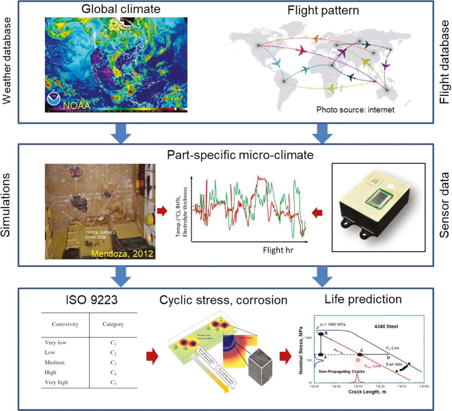
A conceptual representation of the environmental history builder. This includes information extraction from weather database and flight database (top). This information will be used to predict local climate for a specific part or region in the aircraft (middle). Sensor data can provide local data for temperature, RH, TOW, etc., and improve model prediction. The final goal is to integrate the environmental history with structural life prediction models (bottom). Figure on the left in the middle box is taken from Mendoza (2012).

This paper is organized as follows: in Section 2, we discuss the basic model for the development of the environmental history builder by incorporating simple models. An example is presented to show how the model works. This example presents a hypothetical environmental history and should not be regarded as a realistic representation of the Naval operating environment. We then present important conclusions followed by a discussion in Section 3.

2 Modeling prediction of atmospheric corrosion

In an attempt to develop predictive modeling of atmospheric corrosion, three main modeling aspects may be considered: (a) evaporation and condensation of fluid on a metal surface, (b) fluid dynamics of the electrolyte on a metal surface, and (c) rate of corrosion of the metal surface. The rate of evaporation and condensation of fluid on a metal surface depends, to a great extent, on local temperature, local relative humidity (RH), presence of contaminants, surface condition (e.g. surface geometry and slope, surface roughness), and metal thermal properties. The rate of condensation or evaporation can be predicted through a coupled heat and mass transfer model as explained later. The condensation may be in the form of dropwise condensation or filmwise condensation on a metal surface. Both of these mechanisms and their influence on corrosion were studied before (for example, see Tsuru et al., 2004; Dubuisson et al., 2007; Li & Hihara, 2010; Thébault, 2011; Van den Steen, 2016; Palani et al., 2017, among many). The focus of this paper is on the filmwise condensation; meaning, we assume the film thickness will increase or decrease uniformly during condensation and evaporation. The motion of an electrolyte film on a metal surface depends on the geometry of the assembly, surface angle relative to horizontal, and surface roughness. Computational fluid dynamic (CFD) methods can be used to predict motion of an electrolyte layer around the assembly (Palani et al., 2017). CFD simulations are useful tools for predicting electrolyte film evolution and motion especially around complex component parts. In this work, we consider a simple vertical flat plate for which CDF simulations are not required. The development of predictive models for corrosion rate is a more challenging part of the modeling effort. This is due to the fact that the polarization behavior of galvanic couples under thin electrolyte films might be significantly different from the polarization behavior of bulk electrolyte. The variation of electrolyte film thickness during condensation and evaporation makes the problem even more challenging as the appropriate polarization curve for a given film thickness should be adopted. Because of the lack of availability of the polarization curve data under a thin electrolyte, computational models that can predict corrosion under a dynamic electrolyte film become important. On the other hand, in the laboratory, methods for testing atmospheric corrosion often fail to recreate the conditions experienced in the field, as well as the behaviors experienced in field exposures. One method of accelerated lab testing that was utilized to attempt to better simulate field conditions is the use of thin electrolyte layers or droplets. While these tests often provide more realistic conditions, they can be difficult to analyze, particularly measuring the corrosion potential by immersing a reference electrode beneath the electrolyte layer. Because of the complexity of the problem and lack of polarization data under thin electrolyte films, we use an empirical model proposed by Van den Steen et al. (2016). This model, as explained later, relies on film thickness and amount of salt load. The purpose of this paper is to demonstrate the influence of time variation of temperature and RH on the rate of corrosion rather than accurate prediction of corrosion rate. Therefore, the use of complex models for our purpose seems unnecessary.

The basic model used in this paper was proposed by Baklouti et al. (2001) and further adopted by Simillion et al. (2014) and Van den Steen et al. (2016, 2017). We acknowledge that the present model is adopted from these references and is not developed in this paper. The model consists of heat and mass transfer equations for evaporation and condensation, which are coupled through the latent heat. Figure 3 shows a simplified representation of the condensed liquid film on a vertical wall.

Figure 3:

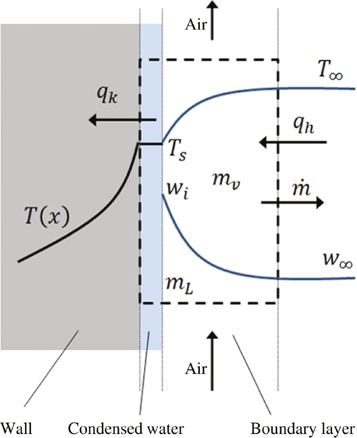
A schematic of the condensed liquid film.

The model geometry consists of a two-dimensional control volume (CV) as shown in Figure 2 with a dashed line. The left boundary of the control volume is in contact with a vertical flat plate with a surface temperature of T_s. The right boundary of the CV is at an ambient temperature of T_∞. We assume that variations of temperature as well as of RH do not change in the vertical direction (i.e. y direction), and variations only happen in the horizontal direction (i.e. x direction in Figure 2). Therefore, we can reduce the problem to a one-dimensional model in which all changes occur in the x direction. We also assume that the temperature of the condensed water is the same as the plate surface temperature T_s. Condensation starts on the plate surface as soon as the surface temperature T_s is below the dew temperature T_dew of the ambient air (Baklouti et al., 2001). The specific mass flux of condensation or vaporization m˙ is a function of the absolute saturated humidity at the plate-air interface w_i, and the absolute humidity of the air w_∞, and can be obtained from:

where k_m is the mass transfer coefficient. The condensation begins when (T_s−T_dew)≤0, and evaporation starts when (T_s−T_dew)>0, where, following the work of Baklouti et al. (2001), these conditions can be expressed as:

It is to be noted that the specific mass flux of condensation or vaporization m˙ in Eqs. (2a)–(2c) is directly related to the rate change of water film thickness on the plate h. This can be realized by considering a uniform thickness film on the plate with known density. If we assume a unit length and unit depth of the plate, then, the time variation of film thickness can be obtained from h˙=m˙/ρw, where ρ_w is the density of the condensed film. The temperature distribution in the plate T(x), can be obtained by solving the heat conduction equation as:

where ρ, c_p, and k are the density, the specific heat capacity, and the thermal conductivity of the plate, respectively. To solve this equation, appropriate boundary conditions on the left and right side of the plate must be imposed. On the left boundary, we can assume that the plate temperature is constant and equal to the ambient temperature T_∞. On the right boundary, the heat flux q_k is supplied to the plate surface, which is the latent heat of condensation/evaporation. The heat released from condensation can increase the plate temperature, and in contrast, the heat absorbed for evaporation can reduce the plate temperature.

A similar equation to Eq. (3) must be solved in the CV to find the distribution of temperature in the air. However, this makes the problem complicated. Instead, we assume that the temperature of air in the CV is constant and equal to the ambient temperature T_∞. Therefore, we can assume a convective heat flux of q_h at the plate-air interface:

where h_c is the heat transfer coefficient. We assumed a constant value for the heat transfer coefficient h_c=10 W/m²K. The model can be further simplified by assuming that the plate temperature remains uniform at all times during the heat transfer process. Therefore, the plate temperature is only a function of time and can be obtained using the lumped capacitance method as (Incropera & DeWitt, 1996):

where T₀ is the plate’s initial temperature, B_i=hL_c/k is the Biot number, and Fo=αt/Lc2 is the Fourier number. α=k/ρc_p is the thermal diffusivity of the plate material, and L_c is the characteristic length of the plate and is assumed to be 3 mm in this analysis.

The absolute humidity of the air w_∞, is calculated from (Cengel & Boles, 2006):

where P is the atmospheric pressure, and p∞s is the vapor pressure of the air calculated from:

In view of getting an idea on how the film thickness influences the corrosion rates, we considered a simple empirical corrosion model proposed by Van den Steen et al. (2016). The model is for iron corrosion; however, our future work includes its development for corrosion models for aluminum. We merely present the final equations for the corrosion current density j as a function of film thickness h; interested readers may refer to Van den Steen et al. (2016) for more details. The corrosion current density is calculated as (Van den Steen et al., 2016):

where j is the corrosion current density in Acm⁻², h is the electrolyte film thickness calculated from the previous section, n is the number of the electrons involved in the charge transfer, F is the Faraday constant, DO2 is the diffusion coefficient of oxygen, and cO2bulk is the bulk concentration of oxygen.

The time of wetness (TOW) is considered as the total time at a temperature higher than 0°C with an RH higher than 80%. We assume a hypothetical variation of temperature and humidity (as shown in Figure 3) and will calculate the variation of film thickness and corrosion rate using this condition. We emphasize that the simulated environment and subsequent results do not necessarily represent the Naval environment. As such, the presented data and results should not be considered as realistic operating environment. The following example is presented to merely demonstrate how the concept of environmental builder works and draw some important conclusions. Figure 4 shows a schematic of a history of variable environmental temperature and RH for 70 h. We divided this history into four events: A, B, C, and D, each having different combinations of temperature and RH, except events A and C, which are identical but different in duration. They also differ in the sense that the events prior to each of these two are different. We should emphasize again that this example might not be realistic. For example, an event with high temperature and high RH may not be realistic. However, the assumed sequence of events yields some important results as presented next.

Figure 4:

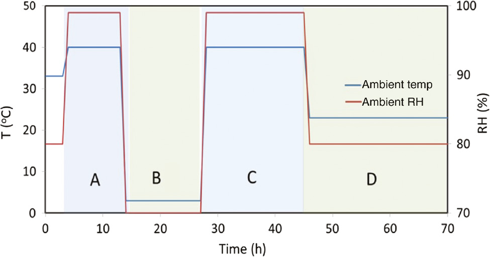
A hypothetical example of variable environment.

Figure 5 shows the results for electrolyte film thickness on the plate, corrosion current density, and corrosion depth. Figure 5A shows the variation of film thickness during each individual event. Event B shows a near-zero film thickness as the temperature and RH during this event drop to small values (see Figure 4). The interesting observation from the results in Figure 5 is the variation of the electrolyte film in event C, which is following event B. Event C is a humid high-temperature event, which is following a low-temperature event B. This may simulate a condition where an aircraft lands to a humid environment after a high-altitude flight. In this way, a cold piece of metal is subjected to humid air. This will result in high accumulation of condensate water on the metal surface. Our simulations show the same result (see Figure 5A). Another important result is the steady state values of film thickness for events A and B as shown in Figure 5A. The steady state value of film thickness for event C is significantly higher than the one for event A even though these two events are identical in temperature and RH. The reason for such difference is the prior event to both of them, each of which following a different event. That is, the event prior to A has a higher temperature and RH compared to event B. This results in a smaller gradient of temperature and RH as we move to event A compared to moving to event C. A smaller gradient in temperature and RH results in a smaller film thickness for event A compared to event C. The higher film thickness, however, may not result in a higher corrosion current density, j, as shown in Figure 5B. It is to be noted that the corrosion current density in Figure 5B is plotted as a dimensionless variable. The relative value of j in different events is more important, for our discussion, to consider than its actual values. Event B has near-zero current density due to near-zero film thickness. Event A has, however, a higher current density compared to event C even though it has a smaller film thickness. This is simply due to the type of corrosion model that we used in this work [i.e. Eq. (8)] and may not be generalized for all types of corrosion and materials.

Figure 5:

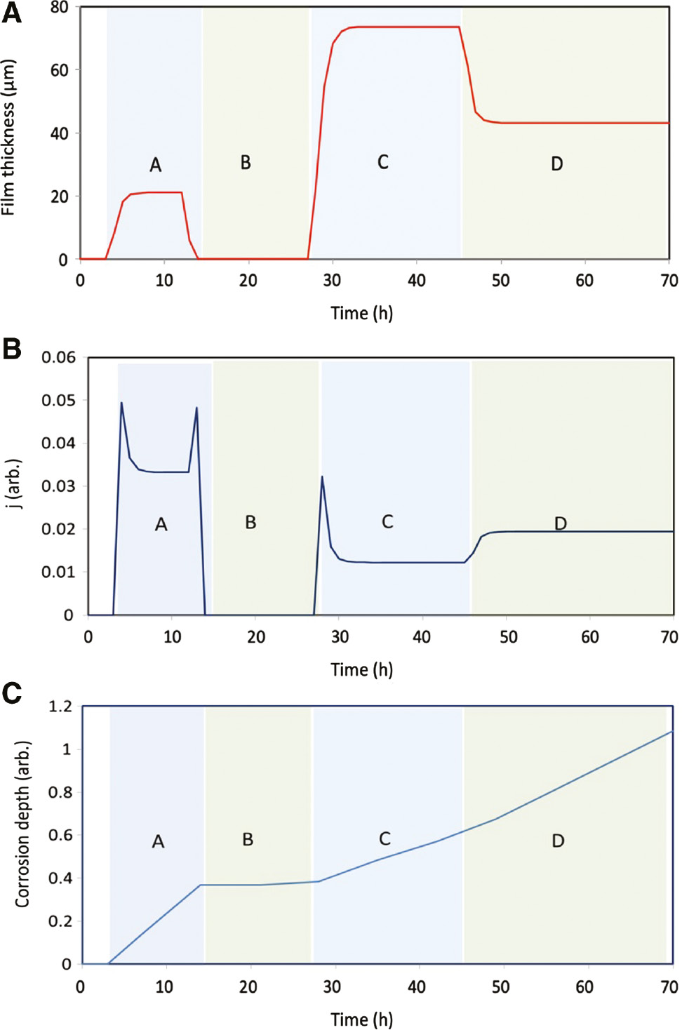
Results for variation of (A) electrolyte film thickness, (B) corrosion current density j, and (C) corrosion depth.

Figure 5C shows the cumulative corrosion depth for all events. The corrosion depth is also plotted in dimensionless form similar to Figure 5B. It is interesting to note that the accumulation of corrosion during event A is about 0.4, while it is about 0.2 during event C. This results in about two times (0.4/0.2=2) higher corrosion accumulation during event A compared to C. It can, however, be seen from Figure 5B that the steady state corrosion current density for event A is about 2.5 (0.035/0.014=2.5) higher than its value in event C. This is due to the fact that event C lasts twice as long as the event A (i.e. event C lasts 16 h, and event A lasts 8 h). The longer the electrolyte film thickness remains on the plate, the higher the accumulation of corrosion depth will be. We can, then, conclude that a combination of the corrosion current density and the duration when the electrolyte film is present on the surface (i.e. TOW) determines the severity of the accumulated corrosion. Therefore, the TOW solely may not be a correct measure of corrosion damage.

Overall, based on the abovementioned simulation, we can draw the following conclusions. First and the most important conclusion is that the sequence of environmental events is important in the estimation of corrosion damage. Events with relatively high temperature and RH, which come after events with low temperature and RH, seem to be the most severe ones. The sequence (or history) effect proves that the predictive models that are based on average temperature and RH may not give a realistic measure of corrosion. Therefore, an environmental history builder should be an integral part of the predictive models of corrosion for applications where the environment is variable as the history effect plays an important role. It is also important to develop predictive models based on both the TOW and the electrolyte film thickness. It is also envisioned that the corrosion damage predictions based on the present model can be integrated with structural damage-predictive models to estimate the damage due to combined mechanical end environmental effects such as corrosion-fatigue or stress corrosion cracking. While a simple model for uniform corrosion damage was adopted in this work, other models for different types of corrosion (e.g. pitting corrosion, stress corrosion cracking, galvanic corrosion, crevice corrosion) can be incorporated into the environmental history builder. This effort is beyond the scope of the present paper. Our future works will include such efforts.

3 Discussion

The Navy environmental conditions are not constant and vary over time. Even in a constant (static) environmental condition, bulk chemistry can be significantly different from local chemistry that is present at the surface of a component or within crevices, pits, and cracks. Therefore, the correlation between bulk and local environment should be fully understood for a given part and environmental conditions. We outlined a plan to develop an environmental history builder in our future effort. The environmental history builder can be used to generate the history of the local climate at the surface of a component based on bulk data. The environmental history builder translates the asset service history (such as stored indoors and outdoors) into a series of scenarios based on the databases of geographical locations. The underlying model that is being used in the environmental history builder is based on both models/simulations and potentially sensor data. Sensor data can provide local data for temperature, RH, TOW, etc., and improve model prediction.

The current model is simple in that it only considers variations in temperature and RH to predict corrosion damage. Several other factors such as salt load, pH, contaminants, ultraviolet light exposure, surface geometry, and part complexity, etc., remain to be included in the model. During atmospheric corrosion, the electrolyte may be in the form of a thin film or droplets or both depending on the interaction of the surface with the environment (Schindelholz & Kelly, 2012). The present model is limited to corrosion under a thin-film electrolyte. Extension of the model to dropwise corrosion is highly desirable especially when localized pitting attack under dry-wet cycling is of concern. Several studies investigated atmospheric corrosion under electrolyte droplets (see, for example, Morton & Frankel, 2014; Risteen et al., 2014; Thomson & Frankel, 2017). Also, a great deal of further work is needed to integrate the environmental history builder with structural life prediction models. The current suite of the models that are available in both the industry and academia for failure prediction of materials under mechanical and environmental loads generally focus on one aspect of the problem. For example, galvanic corrosion models are usually concerned with the calculation of corrosion current density without consideration of the structural impact that the calculated corrosion current density might have on the part. In other words, no conclusion can be made on how much fatigue life, for example, will be influenced for a given corrosion current density. Conversely, models that are used for the prediction of structural failure, such as fracture mechanic models, treat corrosion as a crack starter mechanism by which a pit or crack with assumed size is initiated. These models, alone, are unable to predict structural life under a variable environment, a sequential corrosion fatigue scenario. The motivation for the development of the environmental history builder is to combine these models with corrosion prediction models in an integrated framework so that corrosion can be treated as the structural issue. One of the benefits of this environmental builder is to come up with a corrosion severity index for each individual aircraft based on its environment history. This factor may be used in conjunction with the current deterministic metrics, such as fatigue life expended (FLE) or total life index (TLI), to make informed decisions for operations and maintenance decisions.

The environmental history builder can be integrated with a computational software package such as COMSOL (COMSOL, Inc. Burlington, MA, USA) and Elsyca CorrosionMaster (ELSYCA^®, Inc. c/o ThompsonHine, Atlanta, GA, USA). In this way, electrochemistry simulations can be performed in the computational package for a more refined prediction of the corrosion current density for complex parts. The input to the software packages in the form of varying electrolyte film thickness and environmental conditions can then be provided by the environmental history builder.

References

Baklouti M, Midoux N, Mazaudier F, Feron D. Estimation of the atmospheric corrosion on metal containers in industrial waste disposal. J Hazard Mater 2001; 85: 273–290.10.1016/S0304-3894(01)00238-2Search in Google Scholar
Cengel YA, Boles MA. Thermodynamics: An engineering approach, 5th ed., New York: McGraw-Hill, 2006.Search in Google Scholar
Cooper KR, Ma Y, Wikswo JP, Kelly RG. Simultaneous monitoring of the corrosion activity and moisture inside aircraft lap joints. Corros Eng Sci Technol 2004; 39: 339–345.10.1179/174327804X13217Search in Google Scholar
Demo J, Steiner A, Friedersdorf F, Putic M. Development of a wireless miniaturized smart sensor network for aircraft corrosion monitoring. In: IEEE Aerospace Conference, 6–13 March 2010. NY, NY: IEEE, 2010: 1–9.10.1109/AERO.2010.5446840Search in Google Scholar
Demo J, Friedersdorf F, Andrews C, Putic M. Wireless corrosion monitoring for evaluation of aircraft structural health. In: IEEE Aerospace Conference, 3–10 March 2012. Big Sky, MT: IEEE.10.1109/AERO.2012.6187362Search in Google Scholar
Du ML, Chiang FP, Kagwade SV, Clayton CR. Damage of Al 2024 alloy due to sequential exposure to fatigue, corrosion and fatigue. Int J Fatigue 1998; 20: 743–748.10.1016/S0142-1123(98)00043-7Search in Google Scholar
Dubuisson E, Lavie P, Dalard F, Caire JP, Szunerits S. Corrosion of galvanized steel under an electrolytic drop. Corros Sci 2007; 49: 910–919.10.1016/j.corsci.2006.05.027Search in Google Scholar
DuQuesnay DL, Underhill PR, Britt HJ. Fatigue crack growth from corrosion damage in 7075-T6511 aluminum ally under aircraft loading. Int J Fatigue 2003; 25: 371–377.10.1016/S0142-1123(02)00168-8Search in Google Scholar
Friedersdorf F, Demo J, Averett J. Smart sensor network for aircraft corrosion monitoring. In: 2010 U.S. Army Corrosion Summit, 9–11 February. Huntsville, AL, 2010.Search in Google Scholar
Ganther WD, Paterson DA, Lewis C, Isaacs P, Galea S, Meunier C, Mangeon G, Cole IS. Monitoring aircraft microclimate and corrosion. Procedia Eng 2017; 188: 369–376.10.1016/j.proeng.2017.04.497Search in Google Scholar
Hughes AE, Hinton B, Furman SA, Cole IS, Paterson D, Stonham A, McAdam G, Dixon D, Harris SJ, Trueman A, Hebbron M, Bowden C, Morgan P, Ranson M. Airlife – towards a fleet management tool for corrosion damage. Corros Rev 2007; 25: 275–293.10.1515/CORRREV.2007.25.3-4.275Search in Google Scholar
Incropera FP, DeWitt DP. Fundamentals of heat and mass transfer, 4th ed. New York: Wiley, 1996.Search in Google Scholar
Jones R. Fatigue crack growth and damage tolerance. Fatigue Fract Eng Mater Struct 2014; 37: 463–483.10.1111/ffe.12155Search in Google Scholar
Jones K, Hoeppner DW. The interaction between pitting corrosion, grain boundaries, and constituent particles during corrosion fatigue of 7075-T6 aluminum alloy. Int J Fatigue 2009; 31: 686–692.10.1016/j.ijfatigue.2008.03.016Search in Google Scholar
Li SX, Hihara LH. Atmospheric corrosion initiation on steel from predeposited NaCl salt particles in high humidity atmospheres. Corros Eng Sci Technol 2010; 45: 49–56.10.1179/147842209X12476568584296Search in Google Scholar
Mendoza R. In-service corrosion issues in sustainment of Naval aircraft. In: NAVAIR North Island Advanced Structures Design Group, ASETS Defense Conference 2012.Search in Google Scholar
Molent L. Managing airframe fatigue from corrosion pits – a proposal. Eng Fracture Mech 2015; 137: 12–25.10.1016/j.engfracmech.2014.09.001Search in Google Scholar
Morton SC, Frankel GS. Atmospheric pitting corrosion of AA7075-T6 under evaporating droplets with and without inhibitors. Mater Corros 2014; 65: 351–361.10.1002/maco.201307363Search in Google Scholar
Nickerson WC, Iyyer N, Legg K, Amiri M. Modeling galvanic coupling and localized damage initiation in airframe structures. Corros Rev 2017; 35: 205–224.10.1515/corrrev-2017-0025Search in Google Scholar
Palani S, Rose A, Legg K. Modeling galvanic corrosion behavior of carbon fiber composite/Al 7050 joints under extended exposure. In: Department of Defense – Allied Nations Technical Corrosion Conference, Birmingham, Alabama, August 7–10, 2017, Paper No. 2017-0000.Search in Google Scholar
Risteen BE, Schindelholz E, Kelly RG. Marine aerosol drop size effects on the corrosion behavior of low carbon steel and high purity iron. J Electrochem Soc 2014; 161: C580–C586.10.1149/2.1171412jesSearch in Google Scholar
Schindelholz E, Kelly RG. Wetting phenomena and time of wetness in atmospheric corrosion: a review. Corros Rev 2012; 5–6: 135–207.10.1515/corrrev-2012-0015Search in Google Scholar
Simillion H, Dolgikh O, Terryn H, Deconinck J. Atmospheric corrosion modeling. Corros Rev 2014; 32: 73–100.10.1515/corrrev-2014-0023Search in Google Scholar
Sriraman MR, Pidaparti RM. Crack initiation life of materials under combined pitting corrosion and cyclic loading. J Mater Eng Perform 2010; 19: 7–12.10.1007/s11665-009-9379-9Search in Google Scholar
Thébault F, Vuillemin B, Oltra R, Allely C, Ogle K. Modeling bimetallic corrosion under thin electrolyte films. Corros Sci 2011; 53: 201–207.10.1016/j.corsci.2010.09.010Search in Google Scholar
Thomson MS, Frankel GS. Atmospheric pitting corrosion studies of AA7075-T6 under electrolyte droplets: part I. Effects of droplet size, concentration, composition, and sample aging. J Electrochem Soc 2017; 164: C653–C663.10.1149/2.1051712jesSearch in Google Scholar
Trathan P. Corrosion monitoring systems on military aircraft. In: Proceedings 18th International Conference on Corrosion, Perth 20th–24th November, 2011.Search in Google Scholar
Tsuru T, Tamiya KI, Nishikata A. Formation and growth of micro-droplets during the initial stage of atmospheric corrosion. Electrochim Acta 2004; 49: 2709–2715.10.1016/j.electacta.2004.01.032Search in Google Scholar
Van den Steen N, Simillion H, Dolgikh O, Terryn H, Deconinck J. An integrated modeling approach for atmospheric corrosion in presence of a varying electrolyte film. Electrochim Acta 2016; 187: 714–723.10.1016/j.electacta.2015.11.010Search in Google Scholar
Van den Steen N, Simillion H, Thierry D, Terryn H, Deconinck J. Comparing modeled and experimental corrosion tests on steel. J Electrochem Soc 2017; 164: C554–C562.10.1149/2.0951709jesSearch in Google Scholar
Yang HH, Wang YL, Wang XS, Pan P, Jia DW. Synergistic effect of environmental media and stress on the fatigue fracture behavior of aluminum alloys. Fatigue Fract Eng Mater Struct 2016; 39: 1309–1316.10.1111/ffe.12457Search in Google Scholar
© 2019 Walter de Gruyter GmbH, Berlin/Boston
Articles in the same Issue
- Frontmatter
- In this issue
- Editorial
- International Conference on Stress-Assisted Corrosion Damage V (Hernstein, Austria, July 15–20, 2018)
- General topics