Effect of confined electrolyte volumes on galvanic corrosion kinetics in statically loaded materials
-
Steven A. Policastro
 ,
Carlos M. Hangarter
,
Carlos M. Hangarter

Abstract
This work investigates the effects that the confined volume of atmospheric electrolytes has on the galvanic corrosion kinetics of a martensitic stainless steel alloy, UNS S13800, coupled with UNS A97075 in simulated atmospheric environments at relative humidity values that span the range of operational exposures. Restricted volumes found in thin films and droplets have been shown to control reduction reaction kinetics and are an ongoing challenge to characterize and standardize. This, along with the dynamic and high concentration of aggressive ions found in confined electrolytes, creates a unique corrosion system that requires a multifaceted approach to evaluate varied conditions, compare them with traditional measurements, and more accurately predict galvanic atmospheric corrosion. In this work, corrosion currents in galvanic couples were obtained under two environmental conditions: (1) bulk electrolytes, in a standardized test configuration, with chemistries relevant to atmospheric electrolytes; and (2) deliquesced droplets formed and equilibrated at a given temperature and relative humidity value. The corrosion currents for the same galvanic couple specimens were evaluated, using an atmospheric corrosion model, under a thin film electrolyte while statically loaded and unloaded, at two nominally different locations, e.g. Alexandria, VA, and Miami, FL, on the same date, using recorded weather conditions. The modeled corrosion currents were then compared with the currents obtained from the experimental conditions.
1 Introduction
The electrolytes that form on metal surfaces exposed to the atmosphere are, in general, very different from bulk electrolytes such as seawater or liquids stored in container vessels. These bulk electrolytes, for corrosion purposes, can be considered as reservoirs with nearly constant properties such as component compositions, temperature, and diffusivities. In contrast, thin films and droplets represent the extreme ends of the spectrum of physical forms of electrolyte that can form from atmospheric processes. These electrolytes are characterized by their discrete nature, time-varying component compositions in response to changes in temperature, relative humidity, and deposition rate, and varying transport rates for their components (Stratmann, 1987; Stratmann & Streckel, 1990a,b; Stratmann et al., 1990). The changing properties of the electrolyte also change the susceptibility of the surface to undergo oxidation or catalyze a reduction reaction. For example, a thin film electrolyte that is deposited on a metal surface from a discrete volume of a bulk sodium chloride solution will equilibrate to the ambient temperature and relative humidity (Cole et al., 2003, 2004; Cole & Paterson, 2004, 2007). The water film evaporates in response to the relative humidity in the air, which has a lower activity as compared with water in the bulk solution, and the sodium and chloride concentrations will increase, thereby promoting passive film breakdown, if present on the surface (Zhang & Lyon, 1993; Cai & Lyon, 2005). However, the same increase in ion concentration lowers the saturated solubility of oxygen (Soulie et al., 2015), depleting the availability of dissolved oxygen to participate in the oxygen reduction reaction, even as the thinning electrolyte reduces the diffusion length for dissolved gases to reach the surface (Liu et al., 2017).
In addition to the range of responses of the electrolyte to changing environmental conditions that models of corrosion occurring in thin film or droplet electrolytes need to include, an added complexity occurs when considering galvanic corrosion (Tang et al., 1997). In galvanic corrosion, unlike in other forms of corrosion, the electrochemical properties of the cathodic material are almost as important as the properties of the anodic material in determining the rate of corrosion. The potential difference between the two materials in the given environment provides an indication of the thermodynamic driving force for galvanic corrosion. However, ultimately, it is the magnitude of the corrosion current that determines the amount of anode dissolution. The corrosion rate of the more active material in the galvanic couple is strongly influenced by such environmental conditions as the presence of aggressive anions, which influence anodic reaction kinetics. In many instances, the amount of corrosion damage is also affected by the amount of exposed surface area of the cathode and by the ability of the cathode to support a suitable reduction reaction (Feng & Frankel, 2013; Matzdorf et al., 2013; Policastro et al., 2017).
Of interest to this work are galvanic couples between structural aluminum alloys, such as UNS A92024 and UNS A97075, used on airframes, and high-strength stainless steels, such as UNS S13800 and UNS S17400, which are frequently used as fastener materials.
Based on earlier experimental work (Hangarter & Policastro, 2016), under most relevant environmental conditions, the stainless-steel alloys are more noble than the aluminum alloys and, thus, are assumed to predominantly catalyze reduction reactions of the electrolyte components. Therefore, oxidation at the cathodic stainless steel was not explicitly included in the model. The reduction reactions included in this work are the oxygen reduction reaction, with the four-electron reactions given in equations (1) and (2), for neutral-to-alkaline and acidic environments (Ge et al., 2015), respectively, and the hydrogen evolution reaction, which is given in equation (3).
The aluminum oxidation reaction is given in equation (4). However, once the aluminum cation has crossed the double layer, and depending on the composition of the electrolyte, a large array of possible chemical reactions becomes available (Graedel, 1986, 1989). To reduce the parameter space to a manageable number of reactions and to minimize the approximations needed to estimate reaction rates, only a subset of aluminum hydroxide formation and dissolution chemical reactions were considered in this model. Thus, it should be noted that the reaction shown in equation (7) is only favored if the pH remains above 4. Given the presence of Cl− ions the formation of Al(OH)2Cl is a competitive process that will be considered in a follow-on work (Guseva et al., 2009, 2013). The time constant for Al(OH)2Cl is on the order of 4×10⁻⁶ s−1, and thus, only small concentrations of the chloride product would form over the simulation durations modeled in this report.
The reaction steps for formation/dissolution of Al(OH)3 are shown in equations (4)–(7).
In equations (4)–(7), (s) denotes the solid phase, (aq) denotes the solvated ion, and (p) denotes a precipitate solid.
2 Mathematical model
The geometry of the computational cell is shown in Figure 1. A finite difference approach was used to simulate the time evolution of the diffusion equations for the electrolyte species, and a Crank-Nicolson method (Crank & Nicolson, 1996) was implemented to ensure solution stability. The electrochemical potentials at the alloy nodes were determined as a function of the electrolyte species’ concentration fields at each metal node that bounded the electrolyte. Reaction rates were determined from models of experimentally measured polarization curves. Insulated boundary conditions were used for nodes at y=0 and y=y0. For nodes at z=0 and z=z0, the boundary conditions varied, depending on the species modeled.
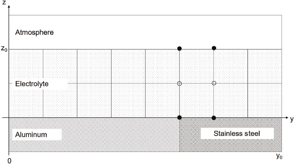
Illustration of a portion of the computational cell. Filled circles indicate boundary nodes. Open circles indicate bulk electrolyte nodes. Only concentration fields at nodes within the electrolyte underwent time evolution.
Figure 2 shows a flowchart of the mathematical model. Input data include temperature, relative humidity, initial electrolyte ion concentrations, and geometry dimensions, to include the initial film thickness.
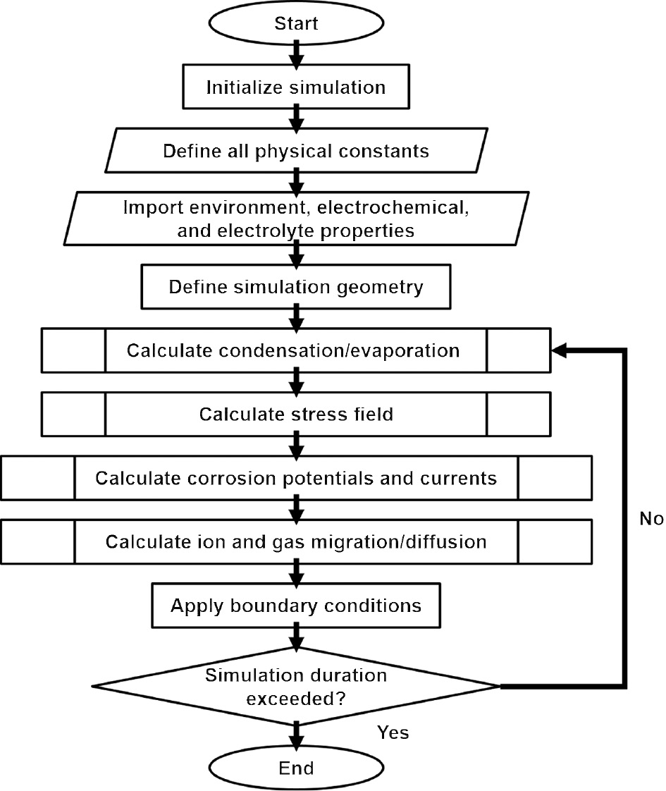
Simulation flowchart.
2.1 Thermodynamics and kinetics of the electrochemical reactions
The electrochemical reactions in this model, i.e. the metal oxidation and various reduction reactions, indexed by the letter k, are treated as outer-sphere electron transfer-limited reactions, and their behavior near the rest potential, obtained from the Nernst equation, (8), is governed by the Butler-Volmer equation, (9).
In equations (8)–(10), R is the ideal gas constant, 8.314 J mol−1 K−1; T is the temperature in K; γ denotes the activity coefficient; c is the concentration of the reactants or products; z is the number of electrons involved in the reaction; F is the Faraday constant, 96,485.3 C mol−1; Eσ is a modification to the rest potential arising from the stress state; β is the asymmetry parameter for the reaction, which provides a measure of the symmetry of the free energy potential curve; η denotes the overpotential applied to drive the reaction away from the rest potential; λ0 denotes the rate constant; and ΔGf,b represent the energy barriers established by the free energy curve for the forward and backward reactions, respectively.
In the case of the oxygen reduction reaction, the low solubility of O2 molecules in water at ambient temperatures and the changing electrolyte composition that can alter the solubility and diffusivity suggest that under certain conditions, electron transfer at the cathodic surface will no longer control the rate of the reduction reaction. Instead, O2 diffusion to the cathodic surface will control the reaction rate. The diffusion-limited oxygen reduction reaction current is obtained from equation (11).
In equation (11),
2.2 Water film evolution
The electrolyte in this model is treated as a continuous film that extends to the edges of the computational cell in the x and y directions, parallel to the surface of the galvanic couple but with varying finite thickness in the z direction. While this runs counter to the generally discrete nature of surface water, it is assumed that corrosion would not occur where there was no electrolyte. The amount of water present in the electrolyte is governed by a simple mass-balance equation.
The mass flux of water across the air-electrolyte interface is, in general, given by an expression with a form similar to equation (13) (Simillion et al., 2016; Van den Steen et al., 2016).
In equation (13), km is a mass transfer coefficient that captures the heat flow to/from the atmosphere to the metal surface to drive the phase transformation between liquid water and water vapor. The individual
In equations (14) and (15), Qaw denotes the ratio of the molar mass of water vapor,
With the assumption that the electrolyte film remains planar during condensation and evaporation and only water molecules participate in the phase change, an analytical expression for the mass flux of water to/from the thin film electrolyte can be obtained from equations (16)–(21) (Lehtinen et al., 1998).
In equations (17)–(22) and (21), A is the surface area of the film,
3 Numerical results and discussion
With the exception of the physical constants, all of the terms in the mathematical model are parameters for which the magnitudes are dependent on the values of various environmental parameters. In many cases, no first principles model exists or would be prohibitively costly to implement during the course of a simulation, but there may be several phenomenological expressions that can be used to estimate the parameter value so choices need to be made on the level of accuracy needed for the calculation. In other cases, expressions for determining parameter values have been obtained from experimental data in the literature.
3.1 Models of electrochemical properties of the anode and cathode
The measured polarization curves used 5 cm×5 cm coupons of UNS A97075 and UNS S13800 cut from panel stock. The surface of each coupon was brought to a 600 grit SiC finish, rinsed with distilled water, cleaned in an ultrasonic bath, and dried with nitrogen just prior to cell assembly. Bulk electrolyte scans were conducted on coupons mounted in Gamry Paracell Kits (Gamry, 2018). The stainless steel coupons were stabilized for 18 h at open circuit potential (Eoc) in 0.6 m NaCl with ambient aeration and polarized cathodically at a scan rate of 0.167 mV/s from Eoc +0.02 V to −1.4VSCE. The aluminum alloy panels were stabilized for 1 h at Eoc and then anodically polarized at a scan rate 0.167 mV/s from Eoc −0.02 V to −0.6VSCE at a rate of 0.167 mV/s. Additional experimental approach details were provided in an earlier paper (Hangarter & Policastro, 2016).
Analysis of the cathodic polarization curve for UNS S13800 provided estimates of the values for the parameters for Butler-Volmer equation and diffusion-limited current densities for the oxygen reduction reactions and hydrogen evolution reaction considered in this model. These parameters are listed in Table 1.
Model parameters used to fit the activation kinetics of the UNS S13800 polarization curve.
| Reaction | β | E 0 (SHE) | z | λ×1014 (s−1) | ΔGf (kJ/mol) | ΔGb (kJ/mol) |
|---|---|---|---|---|---|---|
| ORR – acid | 0.8 | 1.223 | 4 | 1.0 | 290 | 150 |
| ORR – alkaline | 0.9 | 0.401 | 4 | 1.0 | 290 | 140 |
| HER | 0.7 | 0.0 | 2 | 1.0 | – | 160 |
-
HER, Hydrogen evolution reaction; ORR, oxygen reduction reaction; SHE, standard hydrogen electrode.
Examination of the anodic polarization curve for UNS A97075 in 0.6 m NaCl suggested that the corrosion behavior of the alloy could be adequately captured by assuming that the measured corrosion current was obtained from the breakdown of the passivated aluminum surface with little contribution to the current from other alloying elements. Estimates of the necessary parameter values for the Butler-Volmer equation for aluminum oxidation are shown in Table 2.
Model parameters used to fit the activation kinetics of the UNS A97075 polarization curve.
| Reaction | β | E 0 (SHE) | z | λ×1014 (s−1) | ΔGf (kJ/mol) | ΔGb (kJ/mol) |
|---|---|---|---|---|---|---|
| Al oxidation | 0.8 | −0.356 | 3 | 1.0 | 600 | 100 |
-
SHE, Standard hydrogen electrode.
The modeled and measured polarization curves for UNS S13800 are shown in Figure 3A. The modeled and measured polarization curves for UNS A97075 are shown in Figure 3B.
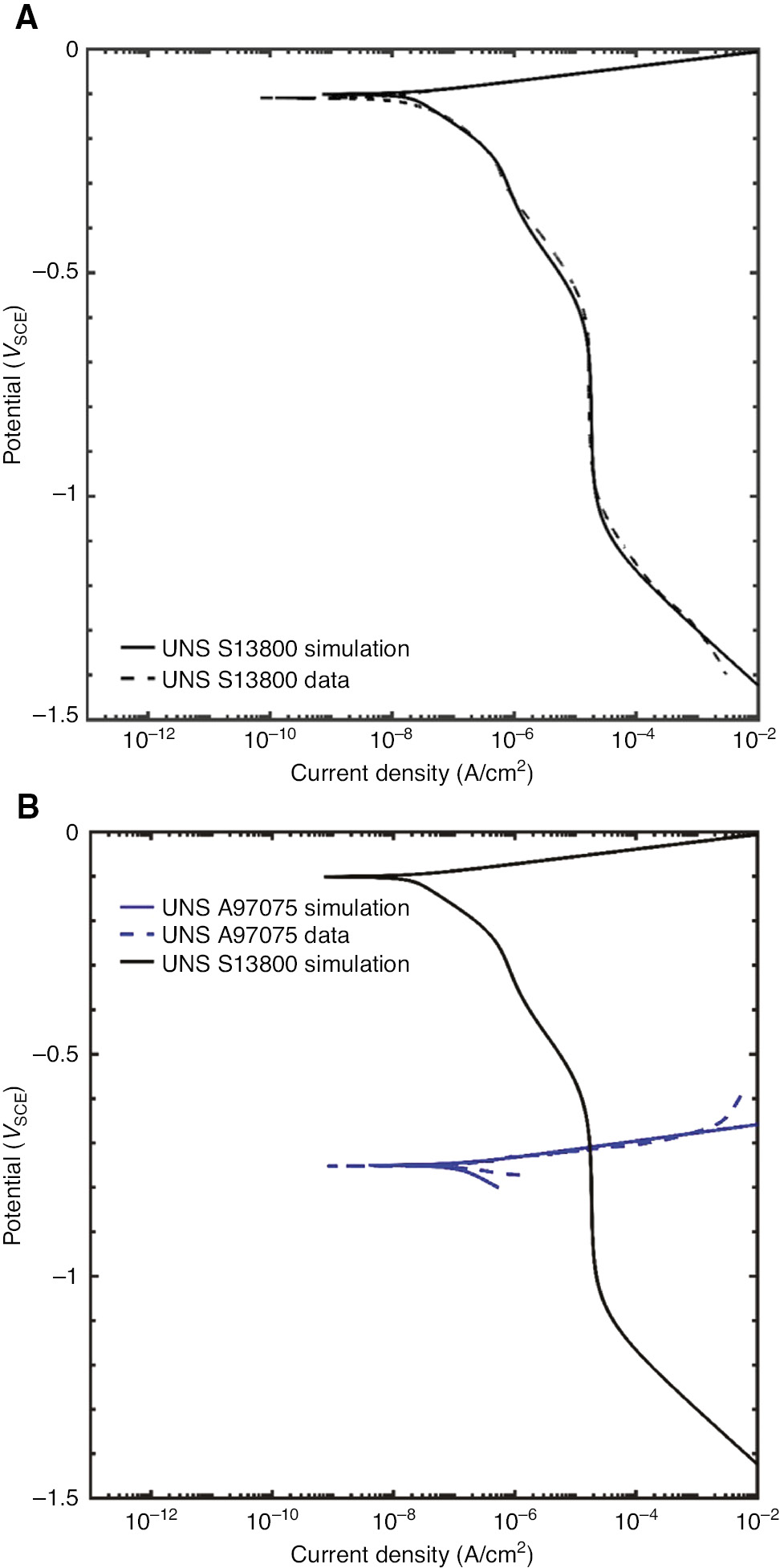
(A) Modeled cathodic polarization curve for UNS S13800 overlaid on experimental data obtained in a 0.6 m NaCl solution. The sample was exposed to the solution for 18 h, and then the potential was scanned from +0.02 V above Eoc to −1.5VSCE at a rate of 0.167 mV/s. (B) Modeled anodic polarization curve for UNS A97075 overlaid on experimental data obtained in a 0.6 m NaCl solution. The sample was exposed to the solution for 1 h, and then the potential was scanned from −0.02 V below Eoc to −0.6VSCE at a rate of 0.167 mV/s.
The electrochemical response of a material has been shown experimentally and through molecular dynamics modeling to be affected by surface stresses. Of interest to this work is how the rest potential of the aluminum alloy can be changed by the application of an applied stress. The modified Nernst potential given in equation (8) allows for the change in potential due to stress. An expression for the term, Eσ, is given in equation (23) (Ma et al., 2016).
where σ0 is the stress field at a given location and Vm is the molar volume of the electrode material. Assuming that the aluminum alloy, as the anode in the galvanic couple, acts as a semi-infinite plate with a hole in the center to accommodate the stainless steel cathode, then with the layout shown in Figure 4, a deformation along the x-axis results in the stress state given by equations (24)–(27).
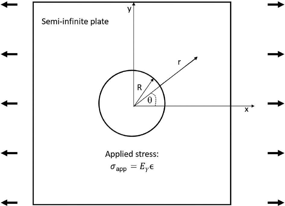
where EY is the Young’s modulus.
Assuming for UNS S97075 that EY=75 GPa, then for 0.1% and 0.2% elongations along the y axis, the calculated stresses and changes in the rest potential are shown in Figure 5A and B, respectively.
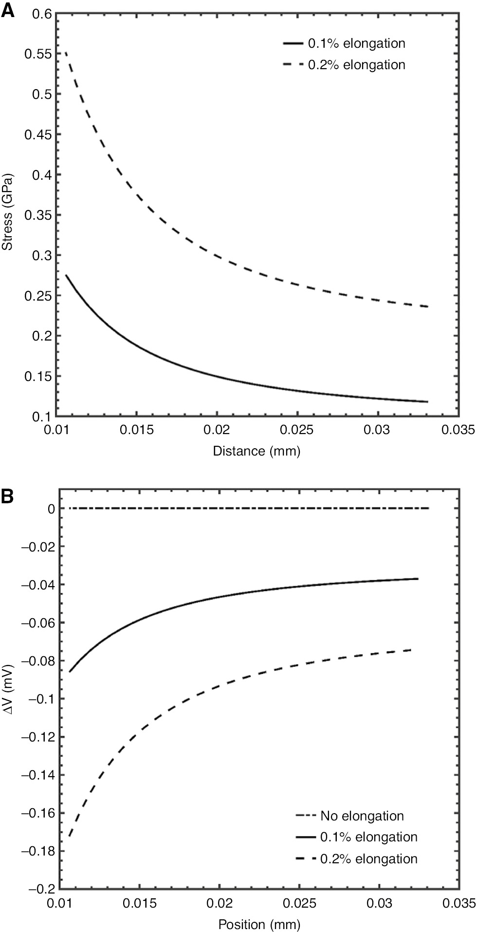
(A) Plot of stresses along the y-axis of the UNS A97075 alloy in the computational cell. (B) Plot of the changes in the rest potential as a function of the stress field.
3.2 Models of solution properties
The number of electrolyte species and chemical reactions included in this simplified solution model still required several additional assumptions and approximations. Water activity was modeled as a function of chloride ion concentration only, even though other solvated ions were present in solution. The dissolved oxygen concentration was assumed to depend only on temperature and dissolved Na+ and Cl− concentrations, and the diffusion coefficient was determined as a function of temperature only. Solution conductivity was modeled with dependencies on temperature and Cl− concentrations only.
Changes in water activity as a function of chloride ion concentration were modeled from data obtained from the literature (Robinson, 1945). Both a polynomial and rational functions provided exact fits to the data, as shown in Figure 6.
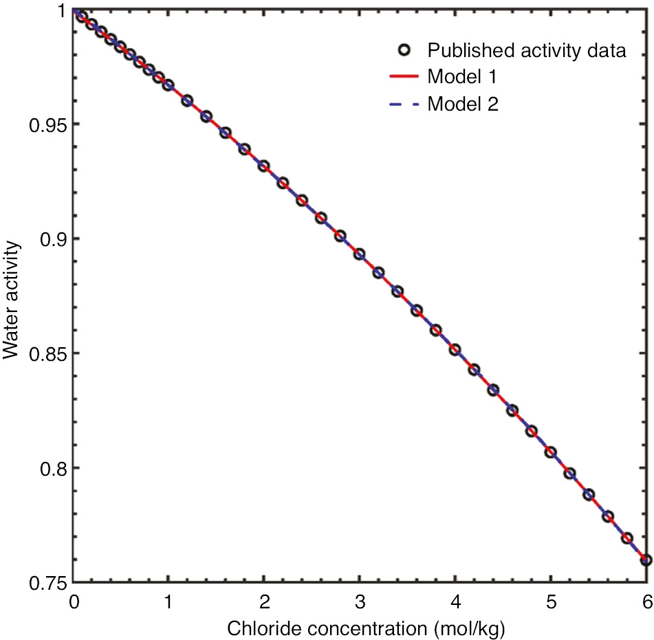
Plot of water activity data as a function of chloride ion concentration and examples of polynomial and rational function fits used for interpolation during the corrosion simulations.
The ambient dissolved oxygen concentration in solution as a function of chloride ion concentration and temperature was modeled using established phenomenological equations (Valderrama et al., 2016). Dissolved O2 concentrations across a range of temperatures and chloride ion concentrations are shown in Figure 7. The O2 diffusivity as a function of temperature is shown in Figure 8 (Han & Bartels, 1996).
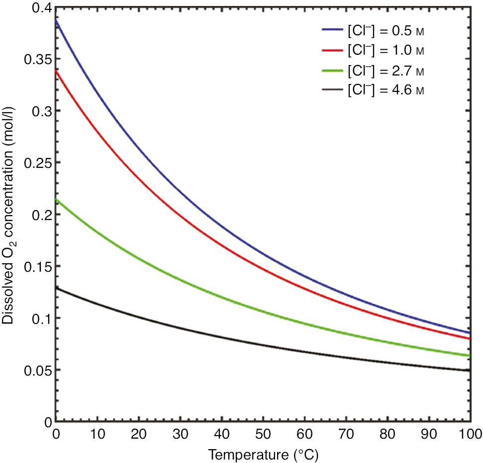
Plots of predicted dissolved oxygen concentrations as a function of chloride ion concentration and temperature.
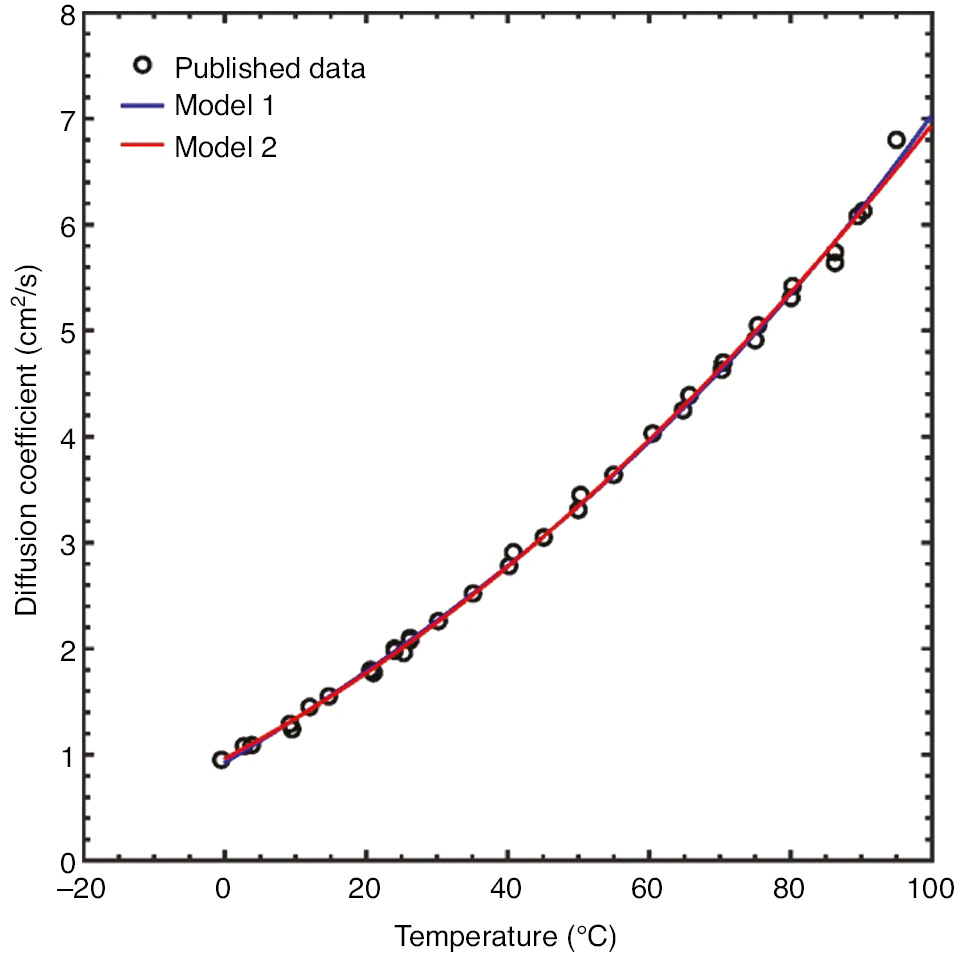
Plot of dissolved O2 diffusion data as a function of temperature overlaid with two fitted models. Model 1 was a rational function model. Model 2 was a polynomial model.
A solution conductivity model, using rational functions, was developed using literature data as a function of temperature and chloride concentration (Shedlovsky, 1932; McCleskey, 2011). Extrapolated conductivities for a range of chloride concentrations and temperatures are shown in Figure 9.
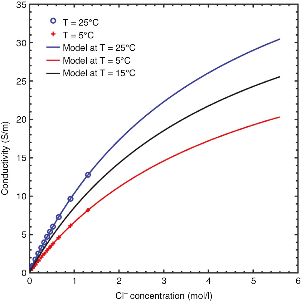
Plot of solution conductivity data at 5°C and 25°C over a range of chloride ion concentrations overlaid with a rational function model at those two temperatures and extrapolated to 15°C.
3.3 Effect of temperature and relative humidity on electrolyte film thickness
Figure 10 provides the range of values for temperature and relative humidity to determine how these factors affected the simulated water film. These values were held constant in time, and the simulated galvanic couple between UNS S13800 and UNS A97075 was initialized with a water film layer 10 μm thick and 65 mm long covering both materials with an initial chloride concentration of 0.5 m. The film was allowed to evolve for 100 s and, at the completion of the simulation, the film thickness values were extracted. A response surface model of the form given in equations (28)–(31) was developed to provide insight into the effect of temperature and relative humidity on the evolution of the water layer thickness, h.
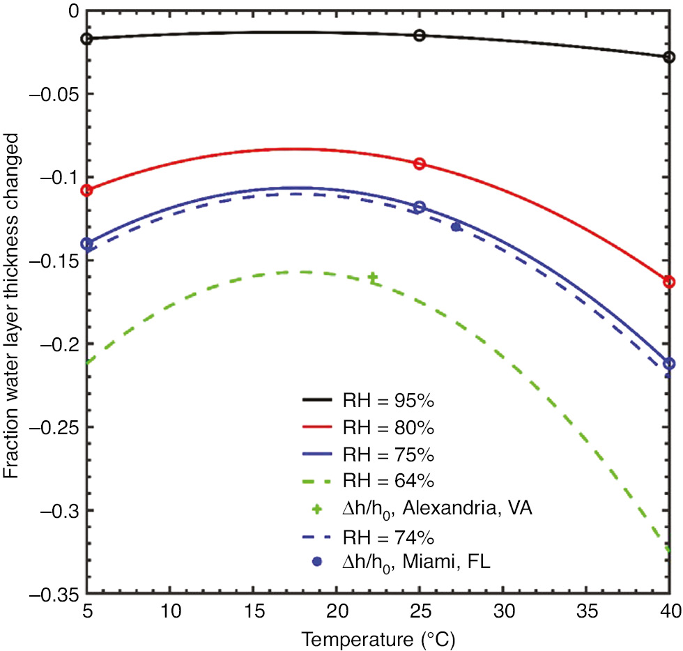
Response surface model of the water layer thickness change for constant temperature and relative humidity values (points) ranging from T=5°C to 40°C and RH values from 75% to 95% with the chloride concentration of 0.5 m. The cross indicates the projected change in water layer thickness for a thin film 0.5 m NaCl electrolyte exposed to the environment on June 27, 2018 in Alexandria, VA, and the filled circle for an identical electrolyte exposed at the same time in Miami, FL.
An examination of Figure 10 suggests that, as expected, the higher temperature, lower relative humidity values lead to the most evaporation, whereas the lower temperatures with higher relative humidity values lead to the least amount of evaporation. The single point values, indicated by the “+” and “*” characters in Figure 10, are the predicted change in water layer thicknesses for simulated electrolyte films exposed to the environmental conditions present in Alexandria, VA, and Miami, FL, on 27 June 2018 (Weather Underground, n.d.).
Plots of the predicted outcomes of galvanic corrosion simulations for these two locations, with the geometry given in Figure 11, are shown in Figure 12. As developed in the model, the interactions among temperature, relative humidity, changing water layer thickness, and changing chloride concentration to produce galvanic corrosion of the aluminum alloy from the stainless steel are quite complex. Even though the electrolyte layer was predicted to thin in both locations, resulting in an apparent increase in the Cl− concentration and thereby suppressing the amount of dissolved oxygen, which would tend to suppress the oxygen reduction reaction, the higher temperature in the Miami location resulted in a prediction of a higher corrosion rate than the Alexandria location.
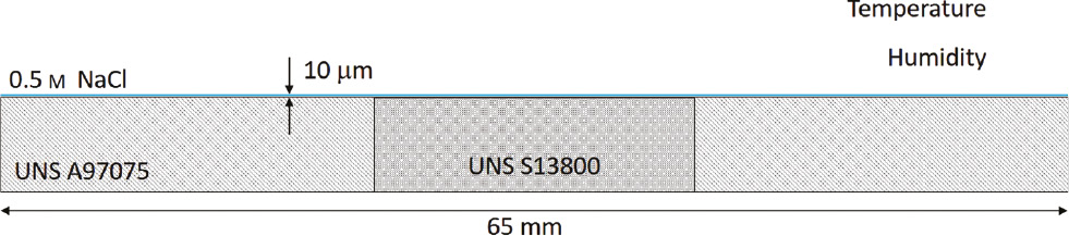
Schematic representation of the simulated galvanic couple exposed to the environmental conditions at two different geographic locations.
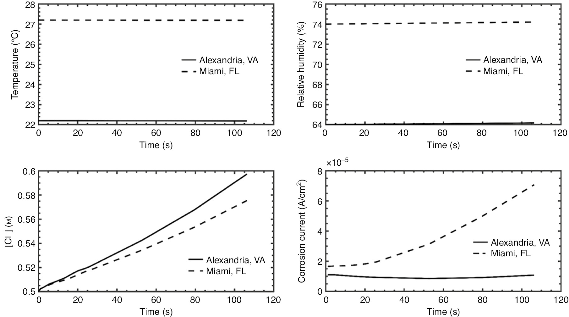
Comparison of temperature and relative humidity at two different locations (top row) with resulting predicted change in Cl− concentration and predicted galvanic corrosion currents (bottom row).
The addition of an elastic stress, resulting from a 0.2% elongation, was predicted to slightly suppress galvanic corrosion by shifting the potential slightly toward the rest potential of the aluminum alloy, and for the Alexandria and Miami locations, the predicted reduction in mass loss due to the applied stress was −0.5% and 0.06%, respectively.
3.4 Comparison with experimental estimates
In previous droplet experiments in a controlled environment chamber with the temperature at 27°C and the relative humidity at 80%, the galvanic corrosion current measured between UNS S13800 and UNS A97075 samples was 1.2×10⁻⁴ A/cm2 (Hangarter & Policastro, 2016). At this temperature and relative humidity combination, an aqueous solution of NaCl is expected to equilibrate to a concentration of 4.7 m. A comparison between simulations at Alexandria and Miami with the experimental values is shown in Figure 13. The simulations suggest that, as expected, the galvanic couple in the Miami environment most closely matched the experimental conditions in the test chamber.
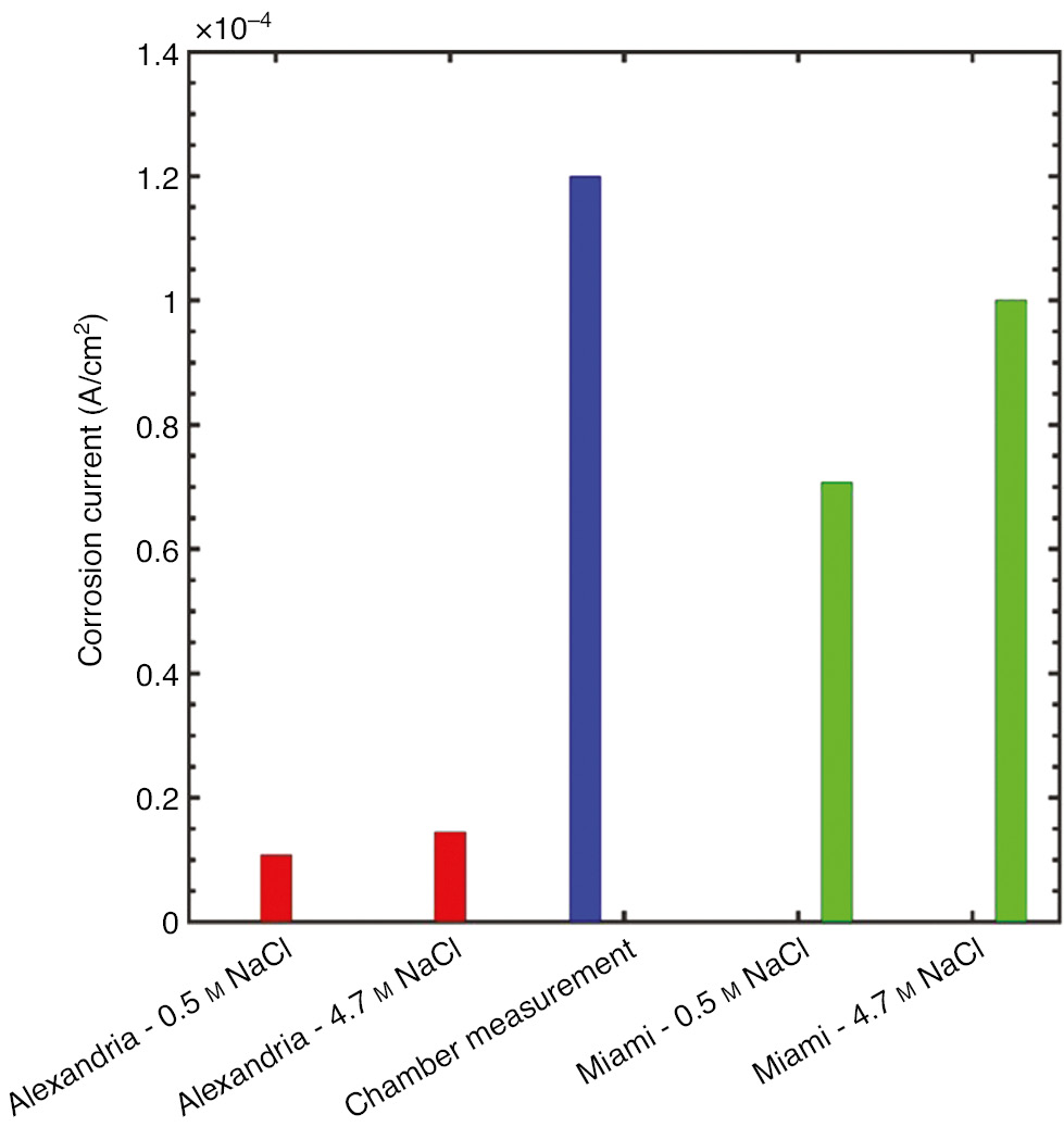
Comparison of simulated corrosion currents with measured corrosion current obtained from droplet measurements in a controlled environment chamber.
4 Conclusions
A new model for galvanic corrosion in relevant atmospheric conditions and with relevant solution chemistries has been developed and validated against experimental measurements obtained from bulk electrolytes and deliquesced droplets. The model, somewhat surprisingly, suggests that temperature plays a large role in driving atmospheric corrosion reactions in galvanic couples, even more so than relative humidity. As long as the chloride concentration is sufficiently high, the passive oxide on the aluminum becomes unstable and temperature effects dominated even as the solution became diluted from additional condensation. The corrosion simulation of the galvanic couple in the Miami environment was shown to match most closely with the chamber corrosion experiments in the lab. Stress effects were shown to have only a small effect on changing the rest potential of the aluminum alloy, but the loading was modeled as elastic deformation only.
While the current model is limited to two-dimensional geometries currently, the approach demonstrates a path forward to develop three-dimensional models that have the capability to predict galvanic corrosion over longer times.
Funding source: Office of Naval Research
Award Identifier / Grant number: N0001418WX00826
Funding statement: Portions of this work were sponsored by the Office of Naval Research, ONR, under Funder Id: http://dx.doi.org/10.13039/100000006, grant/contract no. N0001418WX00826 and under the U.S. Naval Research Laboratory core program. The views and conclusions contained herein are those of the authors and should not be interpreted as necessarily representing the official policies or endorsements, either expressed or implied, of the Office of Naval Research, the U.S. Navy, or the U.S. government.
-
Conflicts of interest: The authors declare to have no conflict of interests.
References
Cai JP, Lyon SB. A mechanistic study of initial atmospheric corrosion kinetics using electrical resistance sensors. Corros Sci 2005; 47: 2956–2973.10.1016/j.corsci.2005.04.011Search in Google Scholar
Cole IS, Paterson DA. Holistic model for atmospheric corrosion – part 5 – factors controlling deposition of salt aerosol on candles, plates and buildings. Corros Eng Sci Technol 2004; 39: 125–130.10.1179/147842204225016949Search in Google Scholar
Cole IS, Paterson DA. Holistic model for atmospheric corrosion – part 7 – cleaning of salt from metal surfaces. Corros Eng Sci Technol 2007; 42: 106–111.10.1179/174327807X196807Search in Google Scholar
Cole IS, Paterson DA, Ganther WD. Holistic model for atmospheric corrosion – part 1 – theoretical framework for production, transportation and deposition of marine salts. Corros Eng Sci Technol 2003; 38: 129–134.10.1179/147842203767789203Search in Google Scholar
Cole IS, Lau D, Paterson DA. Holistic model for atmospheric corrosion – part 6 – from wet aerosol to salt deposit. Corros Eng Sci Technol 2004; 39: 209–218.10.1179/147842204X2880Search in Google Scholar
Crank J, Nicolson P. A practical method for numerical evaluation of solutions of partial differential equations of the heat-conduction type. Adv Comput Math 1996; 6: 207–226.10.1007/BF02127704Search in Google Scholar
Feng Z, Frankel GS. Galvanic test panels for accelerated corrosion testing of coated Al alloys: part 2 – measurement of galvanic interaction. Corrosion 2013; 70: 95–106.10.5006/0907Search in Google Scholar
Gamry. ParaCell Kit for Flat Specimens, 2018. Retrieved from https://www.gamry.com/cells-and-accessories/electrochemical-cells/paracell-kit-for-flat-specimens/. Accessed 21 October, 2018.Search in Google Scholar
Ge X, Sumboja A, Wuu D, An T, Li B, Goh FWT, Andy Hor TS, Zong Y, Liu Z. Oxygen reduction in alkaline media: from mechanisms to recent advances of catalysts. ACS Catal 2015; 5: 4643–4667.10.1021/acscatal.5b00524Search in Google Scholar
Graedel TE. Corrosion-related aspects of the chemistry and frequency of occurrence of precipitation. J Electrochem Soc 1986; 133: 2476–2482.10.1149/1.2108453Search in Google Scholar
Graedel TE. Corrosion mechanisms for aluminum exposed to the atmosphere. J Electrochem Soc 1989; 136: 204C–212C.10.1149/1.2096869Search in Google Scholar
Guseva O, Schmutz P, Suter T, von Trzebiatowski O. Modelling of anodic dissolution of pure aluminium in sodium chloride. Electrochim Acta 2009; 54: 4514–4524.10.1016/j.electacta.2009.03.048Search in Google Scholar
Guseva O, DeRose JA, Schmutz P. Modelling the early stage time dependence of localised corrosion in aluminium alloys. Electrochim Acta 2013; 88: 821–831.10.1016/j.electacta.2012.10.059Search in Google Scholar
Han P, Bartels DM. Temperature dependence of oxygen diffusion in H2O and D2O. J Phys Chem 1996; 100: 5597–5602.10.1021/jp952903ySearch in Google Scholar
Hangarter CM, Policastro SA. Electrochemical characterization of galvanic couples under saline droplets in a simulated atmospheric environment. Corrosion 2016; 73: 268–280.10.5006/2254Search in Google Scholar
Henderson-Sellers B. A new formula for latent heat of vaporization of water as a function of temperature. Q J R Meteorol Soc 1984; 110: 1186–1190.10.1256/smsqj.46624Search in Google Scholar
Lehtinen KEJ, Kulmala M, Vesala T, Jokiniemi JK. Analytical methods to calculate condensation rates of a multicomponent droplet. J Aerosol Sci 1998; 29: 1035–1044.10.1016/S0021-8502(98)80001-3Search in Google Scholar
Liu C, Srinivasan J, Kelly RG. Electrolyte film thickness effects on the cathodic current availability in a galvanic couple. J Electrochem Soc 2017; 164: C845–C855.10.1149/2.1641713jesSearch in Google Scholar
Ma H, Xiong X, Gao P, Li X, Yan Y, Volinsky AA, Su Y. Eigenstress model for electrochemistry of solid surfaces. Sci Rep 2016; 6: 26897.10.1038/srep26897Search in Google Scholar PubMed PubMed Central
Matzdorf CA, Nickerson WC, Rincon Troconis BC, Frankel GS, Li L, Buchheit RG. Galvanic test panels for accelerated corrosion testing of coated Al alloys: part 1 – concept. Corrosion 2013; 69: 1240–1246.10.5006/0905Search in Google Scholar
McCleskey RB. Electrical conductivity of electrolytes found in natural waters from (5 to 90)°C. J Chem Eng Data 2011; 56: 317–327.10.1021/je101012nSearch in Google Scholar
Policastro S, Anderson R, Hangarter C, Horton DJ, Keith JA, Groenenboom MC. Galvanic corrosion of AA7075-T6 caused by doped titanium oxides in a controlled atmospheric environment. Corrosion (General) – 221st ECS Meeting, 2017; 80: 527–539.10.1149/08010.0527ecstSearch in Google Scholar
Robinson RA. The vapour pressures of solutions of potassium chloride and sodium chloride. Trans Proc R Soc N Z. Z. 1945; 75: 203–217.Search in Google Scholar
Shedlovsky T. The electrolytic conductivity of some uni-univalent electrolytes in water at 25°. J Am Chem Soc 1932; 54: 1411–1428.10.1021/ja01343a020Search in Google Scholar
Simillion H, Van den Steen N, Terryn H, Deconinck J. Geometry influence on corrosion in dynamic thin film electrolytes. Electrochim Acta 2016; 209: 149–158.10.1016/j.electacta.2016.04.072Search in Google Scholar
Soulie V, Karpitschka S, Lequien F, Prene P, Zemb T, Moehwald H, Riegler H. The evaporation behavior of sessile droplets from aqueous saline solutions. Phys Chem Chem Phys 2015; 17: 22296–22303.10.1039/C5CP02444GSearch in Google Scholar
Stratmann M. The investigation of the corrosion properties of metals, covered with adsorbed electrolyte layers – a new experimental technique. Corros Sci 1987; 27: 869–872.10.1016/0010-938X(87)90043-6Search in Google Scholar
Stratmann M, Streckel H. On the atmospheric corrosion of metals which are covered with thin electrolyte layers. 1. Verification of the experimental-technique. Corros Sci 1990a; 30: 681–696.10.1016/0010-938X(90)90032-ZSearch in Google Scholar
Stratmann M, Streckel H. On the atmospheric corrosion of metals which are covered with thin electrolyte layers. 2. Experimental results. Corros Sci 1990b; 30: 697–714.10.1016/0010-938X(90)90033-2Search in Google Scholar
Stratmann M, Streckel H, Kim KT, Crockett S. On the atmospheric corrosion of metals which are covered with thin electrolyte layers. 3. The measurement of polarization curves on metal-surfaces which are covered by thin electrolyte layers. Corros Sci 1990; 30: 715–734.10.1016/0010-938X(90)90034-3Search in Google Scholar
Tang IN, Tridico AC, Fung KH. Thermodynamic and optical properties of sea salt aerosols. J Geophys Res Atmos 1997; 102: 23269–23275.10.1029/97JD01806Search in Google Scholar
Valderrama JO, Campusano RA, Forero LA. A new generalized Henry-Setschenow equation for predicting the solubility of air gases (oxygen, nitrogen and argon) in seawater and saline solutions. J Mol Liq 2016; 222: 1218–1227.10.1016/j.molliq.2016.07.110Search in Google Scholar
Van den Steen N, Simillion H, Dolgikh O, Terryn H, Deconinck J. An integrated modeling approach for atmospheric corrosion in presence of a varying electrolyte film. Electrochim Acta 2016; 187: 714–723.10.1016/j.electacta.2015.11.010Search in Google Scholar
Weather Underground. n.d. Retrieved from www.weatherunderground.com. Accessed 29 June, 2018.Search in Google Scholar
Zhang SH, Lyon SB. The electrochemistry of iron, zinc and copper in thin-layer electrolytes. Corros Sci 1993; 35: 713–718.10.1016/0010-938X(93)90207-WSearch in Google Scholar
©2019 Walter de Gruyter GmbH, Berlin/Boston
Articles in the same Issue
- Frontmatter
- In this issue
- Editorial
- International Conference on Stress-Assisted Corrosion Damage V (Hernstein, Austria, July 15–20, 2018)
- General topics
- Building environmental history for Naval aircraft
- Discussion of some recent literature on hydrogen-embrittlement mechanisms: addressing common misunderstandings
- When do small fatigue cracks propagate and when are they arrested?
- Computational modeling of pitting corrosion
- Hydrogen-assisted cracking
- Hydrogen effects on mechanical performance of nodular cast iron
- Ductile-brittle transition temperature shift controlled by grain boundary decohesion and thermally activated energy in Ni-Cr steels
- Hydrogen diffusion in low alloy steels under cyclic loading
- Aluminum alloys
- Initiation and short crack growth behaviour of environmentally induced cracks in AA5083 H131 investigated across time and length scales
- Residual stress affecting environmental damage in 7075-T651 alloy
- Estimation of environment-induced crack growth rate as a function of stress intensity factors generated during slow strain rate testing of aluminum alloys
- Applied topics
- Corrosion modified fatigue analysis for next-generation damage-tolerant management
- Effect of confined electrolyte volumes on galvanic corrosion kinetics in statically loaded materials
- Quasi-static crack propagation in Ti-6Al-4V in inert and aggressive media