A coupled hygro-elastic 3D model for steady-state analysis of functionally graded plates and shells
-
Salvatore Brischetto
 und
Domenico Cesare
und
Domenico Cesare

Abstract
This 3D coupled hygro-elastic model proposes the three-dimensional (3D) equilibrium equations associated with the 3D Fick diffusion equation for spherical shells. The primary unknowns of the problem are the displacements and the moisture content. This coupled 3D exact shell model allows to understand the effects of the moisture field in relation with the elastic field on stresses and deformations in different plates and shells. This model is specifically developed for configurations including functionally graded material (FGM) layers. Four different geometries are analyzed using an orthogonal mixed curvilinear reference system. The main advantage of this reference system for spherical shells is the degeneration of the equations to those for simpler geometries. The solving method is the exponential matrix method in the thickness direction. The closed-form solution is possible because of simply supported sides and harmonic forms for displacements and moisture content. The moisture content amplitudes are directly applied at the top and bottom outer faces through steady-state hypotheses. The final system is based on a set of coupled homogeneous second-order differential equations. The moisture field effects are evaluated for the static analysis in terms of displacement, strain, and stress components. After preliminary validations, used to better understand how to properly define the calculation of the curvature-related terms and FGM properties, four new benchmarks are proposed for several thickness ratios, geometrical data, FGM configurations, and moisture values imposed at the external surfaces. From the results, it is clear the accordance between the uncoupled hygro-elastic model and this new coupled hygro-elastic model when the 3D Fick diffusion law is employed. Both effects connected with the thickness layer and the embedded material are included in the 3D hygro-elastic analyses proposed. The 3D coupled hygro-elastic model is simpler than the uncoupled one because the 3D Fick diffusion law does not have to be separately solved.
1 Introduction
In the framework of aerospace structural analyses, the external environmental conditions become extremely important to be analyzed. Severe temperature and humidity gradients are the classic conditions where these aircraft and spacecraft usually operate [1–4]. In particular, modern aerospace structures can have problems concerning the absorption of humidity from the external air. This phenomenon can create irreversible damages related to the debonding and the mechanical degradation of composite materials, with severe problems related to the safety of aircraft structures. For these reasons, the use of FGMs, whose peculiarity is the continuous variation of its own mechanical, thermal and hygroscopic properties along a given direction, can be relevant. These peculiarities of the FGMs can strongly mitigate all the aforementioned possible damages typical of composite materials.
The scientific and technical literature fulfills various features related to hygro-elastic models for plates and shells embedding FGM layers. Numerical and analytical models (1D, 2D, and 3D approaches) are deeply discussed in this section to better understand the originality of the new proposed model. In all the discussed papers, the moisture field is involved. Two different sections are proposed: in the first one, all the numerical models are deeply described; meanwhile, in the second one, analytical models are shown.
In the context of numerical models, Aria and Friswell [5] showed a hygro-thermal investigation of functionally graded (FG) sandwich microbeams based on Eringen nonlocal elasticity theory where motion equations are derived using Hamilton principle and the first order shear deformation theory (FSDT). The finite element (FE) procedure is based on a five-noded beam element. In the study by Garg et al. [6], the bending analysis of sandwich FGM beams under combined hygrothermomechanical loadings was evaluated. The study was carried out using a FE based on a high order zigzag theory (HOZT). Li and Tang [7] proposed three-directional FGMs to carry out the composition of slender beams. The nonlinear governing equations were developed using the principle of minimum for potential energy. Liu and Mohammadi [8] proposed the bending response of FG nanobeams under hygrothermomechanical loadings. The nonlocal strain gradient theory (NSGT) was implemented to consider both hardening and softening impacts on the system response. Nguyen et al. [9] discussed the hygro-thermal effects on vibration and buckling analyses of FG beams. This work was based on equations of motion obtained from Lagrange equations using a higher-order shear deformation theory. Tang and Ding [10] showed the nonlinear hygro-thermal dynamics of a bi-directionally FG beam where material and hygro-thermal properties gradually change along both thickness and length directions. Dastjerdi et al. [11] proposed a quasi three-dimensional approach for the bending analysis of plates embedding FGMs with porosities. The bending equations were developed using Hamilton principle, and the solution was obtained using a semi-analytical polynomial method. Lee and Kim [12] showed the postbuckling behaviors of FGM plates in hygrothermal environments. The model was based on the FSDT and the von Karman strain-displacement relations, and it was developed using the FE method and the Newton–Raphson technique. Sobhy [13] gave out the bending analysis of sandwich-curved beams with graphene platelets/aluminum (GPLs/Al) nanocomposite face sheets and aluminum honeycomb. The differential quadrature method (DQM), based on a new shear and normal deformation curved beam theory, was employed. Sobhy also [14] presented a three-dimensional asymmetric bending analysis of solid circular and annular plates, made of aluminum matrix reinforced with uniformly distributed GPLs, lying on an elastic medium with different boundary conditions. In-plane magnetic field, transverse external loads, thermal loads, and humid conditions were included. Zhao et al. [15] presented the dynamic analysis of GPL sandwich shallow shells reinforced with FG porous and embedding shape memory alloy (SMA) wires under hygrothermal loadings with general boundary conditions. Dai et al. [16] showed a mechanical model to investigate the coupling between temperature and moisture for a porous FG-carbon nanotube reinforced composite rotating annular plate with variable thickness. Numerical results were achieved by combining the DQM, the Runge–Kutta method, and the Newmark method. Saadaftar and Aghaie-Khafri [17] proposed a rotating FGM cylindrical shell with imperfect surfaces and piezoelectric layers subjected to an axisymmetric hygro-thermo-electro-mechanical loading. The Fourier series expansion method through the longitudinal direction and the DQM along the thickness direction were used to solve governing differential equations. Nie et al. [18] showed the hygro-thermo-electro-mechanical coupling problem of FG piezoelectric structures using the edge-based smoothed point interpolation method (ES-PIM). The basic equations for these structures were derived in the multi-physical field. The resolution of the coupled problem was obtained via ES-PIM and FE method under different hygrothermal conditions.
In the case of exact analytical models, Akbarzadeh and Chen [19] showed analytical solutions for hygrothermal stresses in 1D FG piezoelectric media where material properties varied through the thickness direction. The media were subjected to an external constant magnetic field. Governing equations were written in a unified form in cylindrical and spherical coordinates. Ebrahimi and Barati [20] presented an hygro-thermo-mechanical vibration analysis of FG size-dependent nanobeams exposed to various hygro-thermal loadings. The analysis was performed via a semi-analytical differential transform method. Three hygro-thermal loadings types (uniform, linear, and sinusoidal) were investigated. Ebrahimi and Barati also [21] proposed a study where the combined effects of moisture and temperature on free vibration characteristics of FG nanobeams resting on elastic foundation were investigated. Different refined beam theories, including shear deformations, were involved. Jouneghani et al. [22] investigated the bending behavior of FG nanobeams with internal porosity and subjected to a hygro-thermo-mechanical loading. Eringen nonlocal theory was applied for the numerical study considering a uniform porosity within the nanobeam. The bending response of porous FG Bernoulli–Euler nanobeams under hygrothermomechanical loadings was analyzed by Penna et al. [23]. The governing equations of the problem associated with the local/nonlocal stress and strain-driven gradient models of elasticity were derived using the principle of virtual work. Wang et al. [24] investigated the influence of hygrothermomechanical coupling loadings on buckling behaviors of porous bidirectional FG Timoshenko nanobeams. The governing equations and boundary conditions were derived using a two-phase local strain gradient theory/NSGT employing the principle of virtual work. A hygro-thermal stress analysis of rotating FG graphene/metal sandwich cylindrical shells embedding an auxetic honeycomb core was proposed the study by Allam et al. [25]. The simply supported sandwich shell was spinning about its axial axis with a constant angular speed. Arshid et al. proposed in [26] a study about the vibrational behavior of three-layered cylindrical shells embedding graphene nanoplatelets reinforced composite core and piezo-electro-magnetic face sheets. The whole structure was rested on the visco-Pasternak foundation, and it was exposed to hygro-magneto-electro-thermal loads. Karimiasl et al. [27] investigated the post-buckling behaviors of doubly curved composite shells in a hygro-thermal environment employing multiple scales perturbation methods. Three-phase composite shells with polymer/carbon nanotube/fiber and polymer/GPL/fiber and SMA/matrix were taken into consideration according to the Halpin–Tsai model. Zidi et al. [28] investigated the bending response of an FGM plate resting on elastic foundation and subjected to hygrothermomechanical loadings. Zenkour and Radwan [29] investigated the effects of moisture and temperature on the bending analysis of FG porous plates resting on two-parameter elastic foundation. The effects of transverse normal and shear strains were taken into account. Tang et al. [30] proposed a study where the influence of the hygrothermal effects on center deflections, fundamental natural frequencies, and vibration deflection amplitudes for shells were discussed to understand the service life of polymer matrix composites during operating conditions. In the study by Mudhaffar et al. [31], the bending behavior of an advanced FG ceramic-metal plate subjected to a hygrothermomechanical load and resting on a viscoelastic foundation was studied using a simple higher-order integral shear deformation theory.
All the proposed exact models are related to 1D or 2D theories. For this reason, a 3D hygro-elastic model was developed by Brischetto and Torre in [32] to understand the behavior of shells embedding FGM layers when external moisture conditions were imposed. The present work can be seen as a general extension of the works presented by Brischetto in [33–35] where the mechanical and free vibration analyses of FGM shells were proposed. In the present article, the important novelty with respect to the 3D hygro-elastic shell model proposed by Brischetto and Torre in [32,36] is the full coupling between the displacement field and the hygroscopic field. Therefore, the moisture content profile is directly obtained from the solution of the system, and it is not “a priori” defined. A similar procedure was already used by the authors in [37,38] in the case of full coupling between the displacement field and the thermal field for the 3D bending analysis of composite and FG plates and shells, and in the study by Brischetto and Cesare [39] for the case of full coupling between the displacement field and the hygroscopic field for the 3D bending analysis of classical multilayered composite plates and shells. The Fick diffusion equation [40,41] coupled with 3D equilibrium equations gives a system in mixed curvilinear orthogonal coordinates [42,43]. The system is solved via the exponential matrix method [44,45].
This article is organized in a section containing the theoretical formulation of the 3D coupled hygro-elastic model, a section about results (divided into preliminary validations and new benchmarks) and a section about conclusions where the achieved results are summarized.
2 3D coupled hygro-elastic model for FGM shells
The 3D formulation for full coupled exact hygro-elastic analyses of FGM plates and shells is here presented. This formulation allows hygro-elastic analyses of several geometries such as cylinders, plates, cylindrical panels, and spherical shells. The differences between these four geometries are highlighted in Figure 1. Figure 1 indicates also the mixed curvilinear orthogonal reference system with the origin point located in the left corner. The directions

Geometries in the mixed curvilinear orthogonal reference system.
2.1 Geometrical and constitutive equations
Geometrical relations written in matrix form are here proposed for the coupled 3D hygro-elastic model. The matrix equation is:
where
Each
The curvature shell terms are linear functions of the thickness coordinate
The moisture content
where
Stresses are linked with strains via the 3D Hooke law written for a generic
where the stress vector is
where
In Eq. (6), the six stress components are linked with displacements
2.2 3D equilibrium equations for spherical shells
The equilibrium equations and the 3D Fick diffusion equation for spherical shells are the basic equations of the present coupled formulation. The set of three equilibrium equations for spherical shells written in the matrix form using the mixed curvilinear orthogonal coordinates (
where
The final compact form is:
where subscripts
Eq. (9) is coupled with the 3D Fick diffusion equation for spherical shells in steady-state conditions:
where the diffusion coefficients
2.3 Solution procedure
The resolution of this coupled hygro-elastic problem in a closed form needs the imposition of the Navier conditions for all the main unknowns
Using the Navier form for the unknowns, the boundary conditions are simply-supported sides for all the investigated structures. The capital letters proposed in Eq. (12) are the amplitudes of the unknowns. The
All the primary variables expressed in Eq. (12) are 3D variables because they are functions of
Substituting the primary variables written in the harmonic forms as in Eq. (12), the geometrical relations as in Eq. (1) and the constitutive equations as in Eq. (5) into the governing Eqs. (9) and (10), a global set of four second-order differential equations is obtained. It can be properly transformed into a first-order differential equation system by redoubling the number of unknowns (as stated in [44] and [45]). After all these manipulations, the set of first-order differential equations can be written in a compact matrix form as follows:
where
where
The unknown amplitude vector
Further relationships must be included for interlaminar continuity conditions. They are useful to link the top of the
The interlaminar continuity conditions expressed in Eq. (19) can be easily imposed directly for the amplitudes
where
The boundary conditions for simply supported sides are satisfied for harmonic forms:
Load boundary conditions are imposed on the external faces as follows:
The matrix forms of Eq. (25) are as follows:
and they can be further compacted as follows:
Superscript
It is possible to write
Eq. (30) defines the
Eqs. (29) and (31) can be now compacted in an unique equation as follows:
Matrix
This mathematical formulation is implemented in a Matlab code to evaluate stresses, strains, and displacements along the thickness direction for all the structures presented in the next section and including different FGM configurations (sandwich and single-layered ones).
Once the unknown vector at the bottom of the first fictitious layer (
3 Results
This 3D coupled hygro-elastic shell model here developed is indicated with the acronym 3D-u-
This section is splitted in two different parts: the first subsection is devoted to the validation of the 3D coupled hygro-elastic model for FGM shells by means of comparisons with the past 3D(
Mechanical and hygroscopic properties for the two PVR and for benchmarks (B)
| FGM properties | |
|---|---|
|
|
227.24 |
|
|
65.55 |
|
|
|
|
|
|
|
|
125.83 |
|
|
58.077 |
|
|
|
|
|
|
The volume fraction of the ceramic phase for all the cases proposed (both assessments and benchmarks) is:
where
Bulk and shear moduli of the FGM layer vary in the thickness direction following the Mori-Tanaka model:
where
The moisture expansion coefficient
and the moisture diffusion coefficient
where the dependence on
3.1 Comparisons for validations
Two preliminary validation results (PVRs) are proposed for this new three-dimensional general exact coupled hygro-elastic shell model (3D-u-
Moisture contents, geometrical data, and lamination configurations for the two PVR
| PVR1 | PVR2 | |
|---|---|---|
| Square plate | Cylindrical shell | |
|
|
100 | 1 |
|
|
100 |
|
|
|
25, 10, 2 | 0.2, 0.01 |
|
|
|
|
|
|
|
10 |
|
|
+1.0 | +1.0 |
|
|
+0.5 | +0.5 |
|
|
1 | 1 |
|
|
1 | 1 |
|
|
2.0 | 2.0 |
| Configuration | Single FGM layer | Single FGM layer |
The first preliminary validation results (PVR1) propose a simply supported square plate composed by a single FGM layer. The hygro-elastic material properties are presented in Table 1, and the geometrical parameters are given in the first column of Table 2. Table 3 shows the results of the conducted analyses for different numbers of fictitious layers
Preliminary validation results (PVR1), square plate embedding a single FGM layer. Moisture content applied at the external surfaces. The reference solutions are the 3D uncoupled analytical model and the 3D FE model via Patran and Nastran proposed by Brischetto and Torre [32]
|
|
10 | 50 | 100 | 200 | 300 | |
|---|---|---|---|---|---|---|
|
w [
|
||||||
|
|
3D FEM [32] | 143.3 | 143.3 | 143.3 | 143.3 | 143.3 |
| 3D(
|
151.0 | 141.9 | 141.6 | 141.5 | 141.5 | |
| 3D-u-
|
152.0 | 142.0 | 141.6 | 141.5 | 141.5 | |
|
|
||||||
|
|
3D FEM [32] |
|
|
|
|
|
| 3D(
|
|
|
|
|
|
|
| 3D-u-
|
|
|
|
|
|
|
|
u [
|
||||||
|
|
3D FEM [32] |
|
|
|
|
|
| 3D(
|
|
|
|
|
|
|
| 3D-u-
|
|
|
|
|
|
|
|
|
||||||
|
|
3D FEM [32] |
|
|
|
|
|
| 3D(
|
|
|
|
|
|
|
| 3D-u-
|
|
|
|
|
|
|
|
u [
|
||||||
|
|
3D FEM [32] |
|
|
|
|
|
| 3D(
|
|
|
|
|
|
|
| 3D-u-
|
|
|
|
|
|
|
|
|
||||||
|
|
3D FEM [32] |
|
|
|
|
|
| 3D(
|
|
|
|
|
|
|
| 3D-u-
|
|
|
|
|
|
|
The second preliminary validation results (PVR2) show a simply supported cylindrical shell embedding a single FGM layer. The hygro-elastic material properties are collected in Table 1, and the geometrical parameters are given in the second column of Table 2. Table 4 proposes results for different numbers of fictitious layers
Preliminary validation results (PVR2), cylindrical shell embedding a single FGM layer. Moisture content applied at the external surfaces. The reference solutions are the 3D uncoupled analytical model and the 3D FE model via Patran and Nastran proposed by Brischetto and Torre [32]
|
|
10 | 50 | 100 | 200 | 300 | |
|---|---|---|---|---|---|---|
|
w [
|
||||||
|
|
3D FEM [32] | 411.97 | 411.97 | 411.97 | 411.97 | 411.97 |
| 3D(
|
417.06 | 398.20 | 397.51 | 397.34 | 397.31 | |
| 3D-u-
|
417.80 | 398.20 | 397.52 | 397.35 | 397.31 | |
|
w [
|
||||||
|
|
3D FEM [32] | 279.92 | 279.92 | 279.92 | 279.92 | 279.92 |
| 3D(
|
285.49 | 268.05 | 267.42 | 267.26 | 267.23 | |
| 3D-u-
|
286.30 | 268.06 | 267.42 | 267.26 | 267.23 | |
|
u [
|
||||||
|
|
3D FEM [32] |
|
|
|
|
|
| 3D(
|
|
|
|
|
|
|
| 3D-u-
|
|
|
|
|
|
|
|
u [
|
||||||
|
|
3D FEM [32] |
|
|
|
|
|
| 3D(
|
|
|
|
|
|
|
| 3D-u-
|
|
|
|
|
|
|
|
w [
|
||||||
|
|
3D FEM [32] | 10,128 | 10,128 | 10,128 | 10,128 | 10,128 |
| 3D(
|
10,149 | 10,064 | 10,061 | 10,060 | 10,060 | |
| 3D-u-
|
10,149 | 10,064 | 10,061 | 10,061 | 10,061 | |
|
w [
|
||||||
|
|
3D FEM [32] | 10,123 | 10,123 | 10,123 | 10,123 | 10,123 |
| 3D(
|
10,144 | 10,059 | 10,056 | 10,055 | 10,055 | |
| 3D-u-
|
10,144 | 10,059 | 10,056 | 10,056 | 10,056 | |
|
u [
|
||||||
|
|
3D FEM [32] |
|
|
|
|
|
| 3D(
|
|
|
|
|
|
|
| 3D-u-
|
|
|
|
|
|
|
|
u [
|
||||||
|
|
3D FEM [32] |
|
|
|
|
|
| 3D(
|
|
|
|
|
|
|
| 3D-u-
|
|
|
|
|
|
|
After these PVRs, a number of
3.2 New benchmarks
Four benchmark cases are here proposed. They take into account different characteristics for each case to have a global overview of all the peculiarities. The proposed four benchmarks consider the geometries given in Figure 1. The results obtained in this subsection consider different lamination schemes, FGM properties, and external moisture content impositions.
Moisture contents, geometrical data, and lamination configurations for the four Benchmarks (B).
| B1 | B2 | B3 | B4 | |
|---|---|---|---|---|
| Square plate | Cylinder | Cylindrical shell | Spherical shell | |
|
|
10 | 30 | 30 |
|
|
|
10 | 2
|
|
|
|
|
|
|
|
|
|
|
|
|
|
10 |
|
|
|
10 | 10 | 10 |
|
|
+1.0 | +1.0 | +1.0 | +1.0 |
|
|
0.0 | 0.0 | 0.0 | 0.0 |
|
|
1 | 1 | 0 | 2 |
|
|
1 | 2 | 2 | 2 |
|
|
1.0 | 2.0 | 0.5 | 0.5 |
| Scheme | Single FGM layer | Single FGM layer | Sandwich with FGM core | Sandwich with FGM core |
The first benchmark (B1) considers a square plate with a single FGM layer and simply supported sides. The top of the structure is fully ceramic, and the bottom is fully metallic. All the data used for the hygroelastic analysis are presented in the first column of Table 5. Several thickness ratios are considered to evaluate the effects of geometrical parameters. The thickness ratios vary from

Benchmark 1 (B1), bulk modulus, and volume fraction of the ceramic phase for a square plate embedding a single FGM layer (
Benchmark 1 (B1), square plate embedding a single FGM layer. 3D uncoupled hygro-elastic models [32] vs the 3D coupled hygro-elastic model
|
|
2 | 4 | 10 | 50 | 100 |
|---|---|---|---|---|---|
|
|
|||||
| 3D(
|
0.8000 | 0.8000 | 0.8000 | 0.8000 | 0.8000 |
| 3D(
|
0.5595 | 0.5595 | 0.5595 | 0.5595 | 0.5595 |
| 3D(
|
0.4351 | 0.5197 | 0.5525 | 0.5592 | 0.5594 |
| 3D-u-
|
0.4352 | 0.5197 | 0.5526 | 0.5592 | 0.5594 |
|
v [
|
|||||
| 3D(
|
|
|
|
|
|
| 3D(
|
|
|
|
|
|
| 3D(
|
|
|
|
|
|
| 3D-u-
|
|
|
|
|
|
|
w [
|
|||||
| 3D(
|
1.226 | 2.661 | 6.791 | 34.07 | 68.16 |
| 3D(
|
1.103 | 2.405 | 6.144 | 30.83 | 61.68 |
| 3D(
|
1.008 | 2.336 | 6.113 | 30.83 | 61.67 |
| 3D-u-
|
1.008 | 2.337 | 6.113 | 30.83 | 61.68 |
|
|
|||||
| 3D(
|
|
|
|
|
|
| 3D(
|
|
44.77 | 26.65 | 1.217 | 0.3054 |
| 3D(
|
515.5 | 173.0 | 30.09 | 1.222 | 0.3057 |
| 3D-u-
|
515.5 | 173.0 | 30.09 | 1.222 | 0.3057 |
|
|
|||||
| 3D(
|
|
|
|
|
|
| 3D(
|
|
|
|
|
|
| 3D(
|
|
|
|
|
|
| 3D-u-
|
|
|
|
|
|
|
|
|||||
| 3D(
|
|
|
|
|
|
| 3D(
|
|
3.440 | 4.709 | 1.072 | 0.5379 |
| 3D(
|
19.67 | 12.49 | 5.321 | 1.076 | 0.5384 |
| 3D-u-
|
19.67 | 12.49 | 5.324 | 1.077 | 0.5386 |
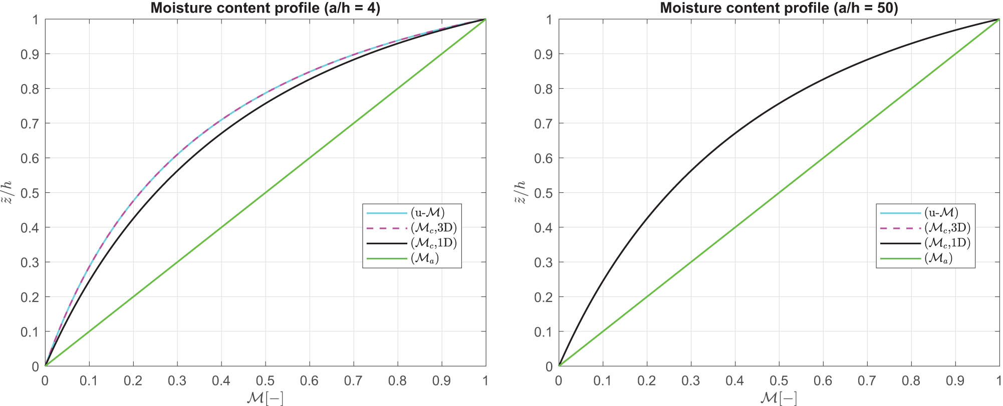
Benchmark 1 (B1), moisture content profile

Benchmark 1 (B1), displacement components, moisture content profile, and stress components for a thick (
The second benchmark (B2) is about a closed cylinder with a single FGM layer and simply supported sides. The metallic and ceramic phases and related mechanical and hygroelastic properties are the same seen in B1 and in Table 1. The geometrical data of the structure are shown in the second column of Table 5. Different thickness ratios are considered to better understand the effects of geometrical parameters. The thickness ratio varies from

Benchmark 2 (B2), bulk modulus and volume fraction of the ceramic phase for a circular cylinder embedding a single FGM layer (
Benchmark 2 (B2), closed cylinder embedding a single FGM layer. 3D uncoupled hygro-elastic models [32] vs the 3D coupled hygro-elastic model
|
|
2 | 4 | 10 | 50 | 100 |
|---|---|---|---|---|---|
|
|
|||||
| 3D(
|
0.5000 | 0.5000 | 0.5000 | 0.5000 | 0.5000 |
| 3D(
|
0.2627 | 0.2627 | 0.2627 | 0.2627 | 0.2627 |
| 3D(
|
0.2439 | 0.2577 | 0.2619 | 0.2627 | 0.2627 |
| 3D-u-
|
0.2439 | 0.2577 | 0.2619 | 0.2627 | 0.2627 |
|
u [
|
|||||
| 3D(
|
|
|
|
|
|
| 3D(
|
|
|
|
|
|
| 3D(
|
|
|
|
|
|
| 3D-u-
|
|
|
|
|
|
|
w [
|
|||||
| 3D(
|
14.96 | 15.14 | 14.73 | 14.33 | 14.27 |
| 3D(
|
9.600 | 9.488 | 9.056 | 8.715 | 8.667 |
| 3D(
|
9.187 | 9.372 | 9.037 | 8.714 | 8.667 |
| 3D-u-
|
9.187 | 9.372 | 9.037 | 8.714 | 8.667 |
|
|
|||||
| 3D(
|
4.442 | 4.370 | 2.346 | 0.5349 | 0.2716 |
| 3D(
|
7.308 | 5.035 | 2.383 | 0.5161 | 0.2605 |
| 3D(
|
7.578 | 5.055 | 2.384 | 0.5161 | 0.2605 |
| 3D-u-
|
7.578 | 5.055 | 2.384 | 0.5161 | 0.2605 |
|
|
|||||
| 3D(
|
12.32 |
|
|
|
|
| 3D(
|
|
|
|
|
|
| 3D(
|
|
|
|
|
|
| 3D-u-
|
|
|
|
|
|
|
|
|||||
| 3D(
|
516.7 | 292.5 | 119.2 | 23.61 | 11.78 |
| 3D(
|
390.8 | 209.0 | 82.62 | 16.12 | 8.025 |
| 3D(
|
381.8 | 207.4 | 82.50 | 16.11 | 8.025 |
| 3D-u-
|
381.8 | 207.4 | 82.50 | 16.11 | 8.025 |

Benchmark 2 (B2), moisture content profile

Benchmark 2 (B2), displacement components, moisture content profile, and stress components for a thick (
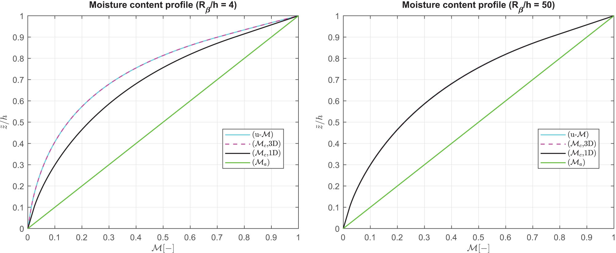
The third benchmark (B3) proposes a sandwich cylindrical shell panel with simply supported sides. The material configuration has a bottom face in Monel (thickness

Benchmarks 3 and 4 (B3–B4), bulk modulus and volume fraction of the ceramic phase for a sandwich cylindrical shell panel and a sandwich spherical shell panel embedding a FGM core (
Benchmark 3 (B3), sandwich cylindrical shell panel embedding a FGM core. 3D uncoupled hygro-elastic models [32] vs the 3D coupled hygro-elastic model
|
|
2 | 4 | 10 | 50 | 100 |
|---|---|---|---|---|---|
|
|
|||||
| 3D(
|
0.5000 | 0.5000 | 0.5000 | 0.5000 | 0.5000 |
| 3D(
|
0.2263 | 0.2263 | 0.2263 | 0.2263 | 0.2263 |
| 3D(
|
0.1100 | 0.1813 | 0.2178 | 0.2260 | 0.2263 |
| 3D-u-
|
0.1100 | 0.1813 | 0.2178 | 0.2260 | 0.2263 |
|
u [
|
|||||
| 3D(
|
0.000 | 0.000 | 0.000 | 0.000 | 0.0000 |
| 3D(
|
0.000 | 0.000 | 0.000 | 0.000 | 0.0000 |
| 3D(
|
0.000 | 0.000 | 0.000 | 0.000 | 0.0000 |
| 3D-u-
|
0.000 | 0.000 | 0.000 | 0.000 | 0.0000 |
|
w [
|
|||||
| 3D(
|
52.486 | 111.71 | 313.64 | 1670.1 | 3364.9 |
| 3D(
|
50.442 | 116.57 | 318.37 | 1653.2 | 3320.1 |
| 3D(
|
47.154 | 113.37 | 316.31 | 1652.8 | 3319.8 |
| 3D-u-
|
47.154 | 113.37 | 316.31 | 1652.8 | 3319.8 |
|
|
|||||
| 3D(
|
|
|
66.489 | 47.729 | 26.056 |
| 3D(
|
|
321.95 |
|
|
|
| 3D(
|
2422.9 | 480.71 |
|
|
|
| 3D-u-
|
2422.9 | 480.71 |
|
|
|
|
|
|||||
| 3D(
|
10,924 | 61,711 | 44,781 | 42,437 | 42,487 |
| 3D(
|
11,090 |
|
|
|
|
| 3D(
|
|
|
|
|
|
| 3D-u-
|
|
|
|
|
|
|
|
|||||
| 3D(
|
0.000 | 0.000 | 0.000 | 0.000 | 0.0000 |
| 3D(
|
0.000 | 0.000 | 0.000 | 0.000 | 0.0000 |
| 3D(
|
0.000 | 0.000 | 0.000 | 0.000 | 0.0000 |
| 3D-u-
|
0.000 | 0.000 | 0.000 | 0.000 | 0.0000 |

Benchmark 3 (B3), moisture content profile

Benchmark 3 (B3), displacement components, moisture content profile, and stress components for a thick (
The last benchmark (B4) considers a sandwich spherical shell panel with simply supported sides. The sandwich lamination, the thickness values of the three layers, and the FGM law are the same seen in B3 (see also Figure 8). The hygro-elastic properties are given in Table 1, and the geometrical data are proposed in the fourth column of Table 5. Table 9 presents some results for different thickness ratios and for different variables. The considerations discussed for the B3 are the same. In Figure 11, it is possible to see the moisture content profile for a moderately thick and a moderately thin sandwich spherical shell configuration. It may be easily noted the fact that the (
Benchmark 4 (B4), sandwich spherical shell panel embedding a FGM core. 3D uncoupled hygro-elastic models [32] vs the 3D coupled hygro-elastic model
|
|
2 | 4 | 10 | 50 | 100 |
|---|---|---|---|---|---|
|
|
|||||
| 3D(
|
0.5000 | 0.5000 | 0.5000 | 0.5000 | 0.5000 |
| 3D(
|
0.2263 | 0.2263 | 0.2263 | 0.2263 | 0.2263 |
| 3D(
|
0.0664 | 0.1492 | 0.2097 | 0.2256 | 0.2262 |
| 3D-u-
|
0.0664 | 0.1492 | 0.2097 | 0.2256 | 0.2262 |
|
v [
|
|||||
| 3D(
|
|
|
|
165.5 | 116.4 |
| 3D(
|
|
|
22.91 | 166.0 | 104.0 |
| 3D(
|
8.931 |
|
30.36 | 165.9 | 104.0 |
| 3D-u-
|
8.931 |
|
30.36 | 165.9 | 104.0 |
|
w [
|
|||||
| 3D(
|
451.5 | 909.6 | 2,454 | 6,323 | 6,380 |
| 3D(
|
348.0 | 763.5 | 1,972 | 4,188 | 3,983 |
| 3D(
|
293.3 | 694.9 | 1,926 | 4,182 | 3,981 |
| 3D-u-
|
293.3 | 694.9 | 1,926 | 4,182 | 3,981 |
|
|
|||||
| 3D(
|
|
|
|
586.86 | 426.57 |
| 3D(
|
|
2494.6 | 897.29 | 620.14 | 390.30 |
| 3D(
|
7524.4 | 3999.2 | 932.31 | 619.62 | 390.19 |
| 3D-u-
|
7524.3 | 3999.2 | 932.31 | 619.62 | 390.19 |
|
|
|||||
| 3D(
|
28,381 | 15,367 | 7733.1 |
|
|
| 3D(
|
11,029 | 4217.1 | 1656.3 |
|
|
| 3D(
|
1946.1 | 1388.9 | 1339.1 |
|
|
| 3D-u-
|
1946.0 | 1388.9 | 1339.1 |
|
|
|
|
|||||
| 3D(
|
89.66 |
|
|
|
|
| 3D(
|
|
|
|
|
|
| 3D(
|
|
|
|
|
|
| 3D-u-
|
|
|
|
|
|
Benchmark 4 (B4), moisture content profile

Benchmark 4 (B4), displacement components, moisture content profile and stress components for a thick (
4 Conclusion
A full coupled hygro-elastic 3D exact shell model for the static analysis of FGM structures has been shown. The moisture content along the thickness direction is evaluated in steady-state conditions. The moisture content profile is a primary variable of the problem together with the displacement components. The 3D Fick diffusion equation for spherical shells allows a moisture content profile that takes into account both thickness layer and material layer effects. The coupled system is solved in a closed form using the exponential matrix method and a layer wise approach. Different results, in terms of displacements, stresses, and moisture content profiles, have been discussed for several thickness ratios, geometrical properties, FGM configurations (sandwich or single layer), and moisture content impositions. These analyses showed a very comforting match between the past 3D uncoupled model that separately solved the 3D Fick diffusion equation and the present 3D full coupled model. The main advantage of this new coupled formulation is the introduction of both thickness and material layer effects using a simpler and more elegant mathematical formulation having a faster convergence: in fact, a reduced number of fictitious layers
-
Funding information: This research received no external funding.
-
Author contributions: Methodology, S.B.; software, S.B.; validation, D.C.; formal analysis, D.C.; investigation, D.C.; data curation, S.B.; writing – original draft, D.C.; writing – review and editing, S.B. All authors have read and agreed to the published version of the manuscript.
-
Conflict of interest: The authors declare no conflict of interest.
References
[1] Bouadi H. Hygrothermal effects on complex moduli of composite laminates [dissertation]. Gainesville (FL): University of Florida; 1998.Suche in Google Scholar
[2] Vodicka R. Accelerated environmental testing of composite materials. DSTO - Aeronautical and Maritime Research Laboratory. DSTOTR-0657. Commonwealth of Australia: Melbourne; 1997. Suche in Google Scholar
[3] Tabrez S, Mitra M, Gopalakrishnan S. Modeling of degraded composite beam due to moisture absorption for wave based detection. CMES - Comput Model Eng Sci. 2007;22(1):77–90. Suche in Google Scholar
[4] Gawin D, Sanavia L. A unified approach to numerical modeling of fully and partially saturated porous materials by considering air dissolved in water. CMES - Comput Model Eng Sci. 2009;53(3):255–302. Suche in Google Scholar
[5] Aria AI, Friswell MI. Computational hygro-thermal vibration and buckling analysis of functionally graded sandwich microbeams. Compos Part B. 2019;165:785–97. 10.1016/j.compositesb.2019.02.028Suche in Google Scholar
[6] Garg A, Chalak HD, Belarbi MO, Zenkour AM. Hygro-thermo-mechanical based bending analysis of symmetric and unsymmetric power-law, exponential and sigmoidal FG sandwich beams. Mechanics Adv Mater Struct. 2022;29(25):4523–45. 10.1080/15376494.2021.1931993Suche in Google Scholar
[7] Li Y, Tang Y. Application of Galerkin iterative technique to nonlinear bending response of three-directional functionally graded slender beams subjected tohygro-thermal loads. Compos Struct. 2022;115481:290. 10.1016/j.compstruct.2022.115481Suche in Google Scholar
[8] Liu B, Mohammadi R. Effects of nonlinear hygro-thermo-mechanical loading on the bending response of nanobeams using nonlocal strain gradient theory. Waves Random Complex Media. 2022:1–17. 10.1080/17455030.2022.2072529Suche in Google Scholar
[9] Nguyen TK, Nguyen BD, Vo TP, Thai HT. Hygro-thermal effects on vibration and thermal buckling behaviors of functionally graded beams. Compos Struct. 2017;176:1050–60. 10.1016/j.compstruct.2017.06.036Suche in Google Scholar
[10] Tang Y, Ding Q. Nonlinear vibration analysis of a bi-directional functionally graded beam under hygro-thermal loads. Compos Struct. 2019;225:111076. 10.1016/j.compstruct.2019.111076Suche in Google Scholar
[11] Dastjerdi S, Malikan M, Dimitri R, Tornabene F. Nonlocal elasticity analysis of moderately thick porous functionally graded plates in a hygro-thermal environment. Compos Struct. 2021;255:112925. 10.1016/j.compstruct.2020.112925Suche in Google Scholar
[12] Lee CY, Kim JH. Hygrothermal postbuckling behavior of functionally graded plates. Compos Struct. 2013;95:278–82. 10.1016/j.compstruct.2012.07.010Suche in Google Scholar
[13] Sobhy M. Differential quadrature method for magneto-hygrothermal bending of functionally graded graphene/Al sandwich-curved beams with honeycomb core via a new higher-order theory. J Sandw Struct Mater. 2021;23:1662–700. 10.1177/1099636219900668Suche in Google Scholar
[14] Sobhy M. 3-D elasticity numerical solution for magneto-hygrothermal bending of FG graphene/metal circular and annular plates on an elastic medium. Eur J MechA Solids. 2021;88:104265. 10.1016/j.euromechsol.2021.104265Suche in Google Scholar
[15] Zhao J, Hu J, Wang T, Li H, Guan J, Liu J, et al. A unified modeling method for dynamic analysis of GPLs-FGP sandwich shallow shell embedded SMA wires with general boundary conditions under hygrothermal loading. Eng Struct. 2022;250:113439. 10.1016/j.engstruct.2021.113439Suche in Google Scholar
[16] Daia T, Yanga Y, Daia HL, Tang H, Lina ZY. Hygrothermal mechanical behaviors of a porous FG-CRC annular plate with variable thickness considering aggregation of CNTs. Compos Struct. 2019;215:198–213. 10.1016/j.compstruct.2019.02.061Suche in Google Scholar
[17] Saadatfar M, Aghaie-Khafri M. Hygrothermal analysis of a rotating smart exponentially graded cylindrical shell with imperfect bonding supported by an elastic foundation. Aerosp Sci Technol. 2015;43:37–50. 10.1016/j.ast.2015.02.012Suche in Google Scholar
[18] Nie B, Ren S, Li W, Zhou L, Liu C. The hygro-thermo-electro-mechanical coupling edge-based smoothed point interpolation method for the response of functionally graded piezoelectric structure under hygrothermal environment. Eng Anal Bound Elem. 2021;130;29–39. 10.1016/j.enganabound.2021.05.004Suche in Google Scholar
[19] Akbarzadeh AH, Chen ZT. Hygrothermal stresses in one-dimensional functionally graded piezoelectric media in constant magnetic field. Compos Struct. 2013;97:317–31. 10.1016/j.compstruct.2012.09.058Suche in Google Scholar
[20] Ebrahimi F, Barati MR. Small-scale effects on hygro-thermo-mechanical vibration of temperature-dependent nonhomogeneous nanoscale beams. Mech Adv Mater Struct. 2017;24:924–36. 10.1080/15376494.2016.1196795Suche in Google Scholar
[21] Ebrahimi F, Barati MR. A unified formulation for dynamic analysis of nonlocal heterogeneous nanobeams in hygro-thermal environment. Appl Phys A. 2016;122:792. 10.1007/s00339-016-0322-2Suche in Google Scholar
[22] Jouneghani FZ, Dimitri R, Tornabene F. Structural response of porous FG nanobeams under hygro-thermo-mechanical loadings. Compos Part B. 2018;152:71–8. 10.1016/j.compositesb.2018.06.023Suche in Google Scholar
[23] Penna R, Feo L, Lovisi G. Hygro-thermal bending behavior of porous FG nano-beams via local/nonlocal strain and stress gradient theories of elasticity. Compos Struct. 2021;263:113627. 10.1016/j.compstruct.2021.113627Suche in Google Scholar
[24] Wang S, Kang W, Yang W, Zhang Z, Li Q, Liu M, et al. Hygrothermal effects on buckling behaviors of porous bi-directional functionally graded micro-/nanobeams using two-phase local/nonlocal strain gradient theory. Eur J Mech/A Solids. 2022;94;104554. 10.1016/j.euromechsol.2022.104554Suche in Google Scholar
[25] Allam MNM, Radwan AF, Sobhy M. Hygrothermal deformation of spinning FG graphene sandwich cylindrical shells having an auxetic core. Eng Struct. 2022;251:113433. 10.1016/j.engstruct.2021.113433Suche in Google Scholar
[26] Arshid E, Soleimani-Javid Z, Amir S, DinhDuc N. Higher-order hygro-magneto-electro-thermo-mechanical analysis of FG-GNPs reinforced composite cylindrical shells embedded in PEM layers. Aerosp Sci Tech. 2022;126:107573. 10.1016/j.ast.2022.107573Suche in Google Scholar
[27] Karimiasla M, Ebrahimia F, Akgözb B. Buckling and post-buckling responses of smart doubly curved composite shallow shells embedded in SMA fiber under hygro-thermal loading. Compos Struct. 2019;223:110988. 10.1016/j.compstruct.2019.110988Suche in Google Scholar
[28] Zidi M, Tounsi A, Houari MSA, Bedia EAA, AnwarBég O. Bending analysis of FGM plates under hygro-thermo-mechanical loading using a four variable refined plate theory. Aerosp Sci Tech. 2014;34:24–34. 10.1016/j.ast.2014.02.001Suche in Google Scholar
[29] Zenkour AM, Radwanc AF. Bending response of FG plates resting on elastic foundations in hygrothermal environment with porosities. Compos Struct. 2019;213:133–43. 10.1016/j.compstruct.2019.01.065Suche in Google Scholar
[30] Tang H, Dai HL, Du Y. Effect of hygrothermal load on amplitude frequency response for CFRP spherical shell panel. Compos Struct. 2022;281:114978. 10.1016/j.compstruct.2021.114978Suche in Google Scholar
[31] Mudhaffar IM, Tounsi A, Chikh A, Al-Osta MA, Al-Zahrani MM, Al-Dulaijan SU. Hygro-thermo-mechanical bending behavior of advanced functionally graded ceramic metal plate resting on a viscoelastic foundation. Structures. 2021;33:2177–89. 10.1016/j.istruc.2021.05.090Suche in Google Scholar
[32] Brischetto S, Torre R. 3D stress analysis of multilayered functionally graded plates and shells under moisture conditions. Appl Sci. 2022;12:512. 10.3390/app12010512Suche in Google Scholar
[33] Brischetto S. A general exact elastic shell solution for bending analysis of funcionally graded structures. Compos Struct. 2017;175:70–85. 10.1016/j.compstruct.2017.04.002Suche in Google Scholar
[34] Brischetto S. A 3D layer-wise model for the correct imposition of transverse shear/normal load conditions in FGM shells. Int J Mech Sci. 2018;136:50–66. 10.1016/j.ijmecsci.2017.12.013Suche in Google Scholar
[35] Brischetto S. Exact elasticity solution for natural frequencies of functionally graded simply-supported structures. CMES - Comput Model Eng Sci. 2013;95:391–430. Suche in Google Scholar
[36] Brischetto S, Torre R. 3D hygro-elastic shell model for the analysis of composite and sandwichstructures. Compos Struct. 2022;285:115162. 10.1016/j.compstruct.2021.115162Suche in Google Scholar
[37] Brischetto S, Torre R, Cesare D. Three dimensional coupling between elastic and thermal fields in the static analysis of multilayered composite shells. CMES Comput Model Eng Sci. 2023;136:2551–94. 10.32604/cmes.2023.026312Suche in Google Scholar
[38] Brischetto S, Cesare D, Torre R. A layer-wise coupled thermo-elastic shell model for three-dimensional stress analysis of functionally graded material structures. Technologies. 2023;11:35. 10.3390/technologies11020035Suche in Google Scholar
[39] Brischetto S, Cesare D. Hygro-elastic coupling in a 3D exact shell model for bending analysis of layered composite structures. J Compos Sci. 2023;7:1–27. 10.3390/jcs7050183Suche in Google Scholar
[40] Özişik MN. Heat conduction. New York (NY), USA: John Wiley & Sons, Inc; 1993. Suche in Google Scholar
[41] Povstenko Y. Fractional thermoelasticity. Cham, Switzerland: Springer International Publishing; 2015. 10.1007/978-3-319-15335-3Suche in Google Scholar
[42] Moon P, Spencer DE. Field Theory Handbook. Including Coordinate Systems, Differential Equations and Their Solutions. Berlin, Germany: Springer-Verlag; 1988. 10.1007/978-3-642-83243-7Suche in Google Scholar
[43] Mikhailov MD, Özişik MN. Unified analysis and solutions of heat and mass diffusion. New York (NY), USA: Dover Publications Inc.; 1984. Suche in Google Scholar
[44] Boyce WE, DiPrima RC. Elementary differential equations and boundary value problems. New York (NY), USA: John Wiley & Sons, Ltd.; 2001. Suche in Google Scholar
[45] Open document. Systems of differential equations. [Internet]. http://www.math.utah.edu/gustafso/. [Accessed on 30 May 2013].Suche in Google Scholar
[46] Reddy JN, Cheng ZQ. Three-dimensional thermomechanical deformations of functionally graded rectangular plates. Eur J Mech/A Solids. 2001;20:841–55. 10.1016/S0997-7538(01)01174-3Suche in Google Scholar
© 2023 the author(s), published by De Gruyter
This work is licensed under the Creative Commons Attribution 4.0 International License.
Artikel in diesem Heft
- Research Articles
- Investigation of differential shrinkage stresses in a revolution shell structure due to the evolving parameters of concrete
- Multiphysics analysis for fluid–structure interaction of blood biological flow inside three-dimensional artery
- MD-based study on the deformation process of engineered Ni–Al core–shell nanowires: Toward an understanding underlying deformation mechanisms
- Experimental measurement and numerical predictions of thickness variation and transverse stresses in a concrete ring
- Studying the effect of embedded length strength of concrete and diameter of anchor on shear performance between old and new concrete
- Evaluation of static responses for layered composite arches
- Nonlocal state-space strain gradient wave propagation of magneto thermo piezoelectric functionally graded nanobeam
- Numerical study of the FRP-concrete bond behavior under thermal variations
- Parametric study of retrofitted reinforced concrete columns with steel cages and predicting load distribution and compressive stress in columns using machine learning algorithms
- Application of soft computing in estimating primary crack spacing of reinforced concrete structures
- Identification of crack location in metallic biomaterial cantilever beam subjected to moving load base on central difference approximation
- Numerical investigations of two vibrating cylinders in uniform flow using overset mesh
- Performance analysis on the structure of the bracket mounting for hybrid converter kit: Finite-element approach
- A new finite-element procedure for vibration analysis of FGP sandwich plates resting on Kerr foundation
- Strength analysis of marine biaxial warp-knitted glass fabrics as composite laminations for ship material
- Analysis of a thick cylindrical FGM pressure vessel with variable parameters using thermoelasticity
- Structural function analysis of shear walls in sustainable assembled buildings under finite element model
- In-plane nonlinear postbuckling and buckling analysis of Lee’s frame using absolute nodal coordinate formulation
- Optimization of structural parameters and numerical simulation of stress field of composite crucible based on the indirect coupling method
- Numerical study on crushing damage and energy absorption of multi-cell glass fibre-reinforced composite panel: Application to the crash absorber design of tsunami lifeboat
- Stripped and layered fabrication of minimal surface tectonics using parametric algorithms
- A methodological approach for detecting multiple faults in wind turbine blades based on vibration signals and machine learning
- Influence of the selection of different construction materials on the stress–strain state of the track
- A coupled hygro-elastic 3D model for steady-state analysis of functionally graded plates and shells
- Comparative study of shell element formulations as NLFE parameters to forecast structural crashworthiness
- A size-dependent 3D solution of functionally graded shallow nanoshells
- Special Issue: The 2nd Thematic Symposium - Integrity of Mechanical Structure and Material - Part I
- Correlation between lamina directions and the mechanical characteristics of laminated bamboo composite for ship structure
- Reliability-based assessment of ship hull girder ultimate strength
- Finite element method on topology optimization applied to laminate composite of fuselage structure
- Dynamic response of high-speed craft bottom panels subjected to slamming loadings
- Effect of pitting corrosion position to the strength of ship bottom plate in grounding incident
- Antiballistic material, testing, and procedures of curved-layered objects: A systematic review and current milestone
- Thin-walled cylindrical shells in engineering designs and critical infrastructures: A systematic review based on the loading response
- Laminar Rayleigh–Benard convection in a closed square field with meshless radial basis function method
- Determination of cryogenic temperature loads for finite-element model of LNG bunkering ship under LNG release accident
- Roundness and slenderness effects on the dynamic characteristics of spar-type floating offshore wind turbine