In-plane nonlinear postbuckling and buckling analysis of Lee’s frame using absolute nodal coordinate formulation

3.1 Omar-Shabana beam element (OmSh)

The standard two-dimensional shear deformable ANCF beam element in which elastic forces are derived using the GCM approach is abbreviated as “OmSh” in this study [47]. For this OmSh element, the assumed displacement field in the global coordinate system is defined as follows:

Then, the position vector of an arbitrary point on the beam is obtained by r = S ( x ) e , where x is the material coordinate vector in the straight configuration and e is the vector of nodal coordinates given by

The element has two nodes, while the position vector r i and the two gradient vectors r x i = ∂ r i / ∂ x and r y i = ∂ r i / ∂ y , i = 1 , 2 are used as DOFs, where x and y are the material coordinates in the straight configuration. The matrix of shape functions is given by

where I is the identity matrix and s i ( i = 1 , 2 , … , 6 ) are shape functions:

where ξ and η are the dimensionless bi-normalized element coordinates and l is the length of the beam element in the initial reference configuration. The bi-normalized coordinates are ξ = x / l and η = y / l , where 0 ≤ x ≤ l and − h / 2 ≤ y ≤ h / 2 , h is the height of the element. According to the GCM approach, the matrix of the position vector gradients (Jacobian matrix) or the deformation gradient is given by

where X = S ( x ) e 0 represents the element parameters in the initial reference configuration, J e = ∂ r / ∂ x and J 0 = ∂ X / ∂ x . The Green–Lagrange strain matrix is obtained as follows:

where I is the identity matrix and the strain in Voigt is written as follows:

where ε x x , ε y y , and ε x y represent the axial, transverse, and shear strains, respectively. For the linearly elastic material, the strain energy is calculated using the following relation:

where det ( J 0 ) indicates the determinant of J 0 , V indicates straight configuration volume, and E m is the matrix of elastic coefficients. The plane stress assumption is adopted as follows:

where E is Young’s modulus and ν is Poisson’s ratio. The stress vector from the mechanics definition is calculated as follows:

The elastic force can be obtained by differentiating the elastic energy with respect to the nodal vector as follows:

Then, the tangential stiffness matrix will be obtained by derivation of elastic force by the nodal coordinate vector as follows:

where the numbers represent the position of stress and strain component in the corresponding vectors.

3.2 Omar–Shabana beam element with Strain Split Method (OS-SSM)

SSM was originally proposed by Patel and Shabana in order to alleviate the locking problem present in the standard Omar–Shabana ANCF beam element [48]. For the SSM approach, the assumed displacement field equations remain as shown in Eq. (1). This approach is abbreviated as “OS-SSM” in this study. Locking alleviation was achieved by decoupling the higher-order strain terms found in the axial strain and the transverse strain. In this approach, the position field of the beam element is defined as follows:

where the superscript c represents the centerline of the beam and the matrix of the position vector gradients is defined as follows:

where J c represents terms belonging to the centerline of the beam and J k represents terms belonging to higher-order terms associated with the shear deformation and curvature of the beam element. The Green–Lagrange strain tensor is defined as ε = ε c + ε k , and the two strains are given as follows:

The second Piola–Kirchoff stress in the Voigt form is expressed as σ v = E c ε v c + E k ε v k , where strains are also written in Voigt form. In addition, E k = diag ( E , E , μ k s ) while utilizing the plane strain assumption E c is defined as follows:

where λ and μ are Lamé parameters, E is Young’s modulus, and ν is Poisson’s ratio, whereas k s = 10 ( 1 + ν ) / ( 12 + 11 ν ) is the shear correction coefficient. The strain energy is given by

The strain energy in the form of stress and strain vector is shown in the above equation. Then, the elastic force and tangential stiffness matrix are calculated using the formulation shown in Section 3.1. Complete derivation for SSM and further details about how to use it for curved geometries can be found in the study of Patel and Shabana [48].

3.3 Enhanced continuum mechanics formulation (OS-EnCM)

The standard Omar–Shabana (OmSh) beam element has been found to have Poisson locking because of the axial strain and transverse strain coupling in the energy formulation. To avoid this, Gerstmayr et al. [49] proposed the method known as enhanced continuum mechanics formulation in which the strain energy is calculated in two parts. In this way, the Poisson effect is excluded in the transverse direction, and the Poisson effect is included only in the beam centerline. This approach is utilized in the Omar–Shabana beam element framework, hence, abbreviated as “OS-EnCM.” The assumed displacement field equation for this approach is shown in Eq. (1). The formulation for strain energy is as follows:

where b is the thickness of the element; the first part excludes the Poisson effect with the help of the modified matrix of elastic coefficients given as follows:

where G = E / 2 ( 1 + ν ) is the shear modulus. And, the matrix of elastic coefficients for the second part is formulated as follows:

which includes the Poisson effect in the transverse direction. Then, the elastic force vector is given as follows:

where σ 0 = D 0 ε and σ v = D v ε . The tangential stiffness matrix is given as follows:

where the numbers show the components in the corresponding vectors. The total tangential stiffness matrix is the sum of the two as follows:

3.4 Higher order beam element (HOBE)

In the locking alleviation article, Patel and Shabana also proposed a new two-dimensional HOBE with 16 DOFs [48]. The HOBE adopts cubic interpolation in the longitudinal direction and quadratic interpolation in the transverse direction. The higher order interpolation allows capturing the complex deformation modes and also allows curvature level continuity on the elemental nodes. The transverse strain does not remain constant, thus allowing the easing of the Poisson locking, especially in the large deformation analysis. This element can also be directly derived as a two-dimensional subset from the three-dimensional HOBE proposed by Shen et al. [50], which was later found to be useful in the study of lateral buckling by Orzechowski and Shabana [51]. For HOBEs, the assumed displacement field in the global coordinate system is defined as follows:

The element nodal coordinate vector for the HOBE is defined as follows:

Correspondingly, the element has the second-order gradient r yy i = ∂ 2 r i / ∂ y 2 , i = 1 , 2 , as the nodal DOFs, besides r i , r x i , r y i i = 1 , 2 as in the standard element (OmSh). The matrix of shape functions is defined as follows:

where I is the identity matrix and s i , i = 1 , 2 , … , 8 , are shape functions given as follows:

The strain energy, elastic force, and stiffness matrix derivation follow the GCM-based approach. The strain energy for HOBE is given by

Furthermore, elastic force and tangential stiffness matrix are calculated, as shown in Section 3.1.

3.5 Slope discontinuity modeling using ANCF

As the gradient is not continuous at the rigid joint of Lee’s frame, it requires special attention. Therefore, the technique to model the slope discontinuity using ANCF finite element is briefly described here. The utilization of a constant coordinate transformation matrix to deal with the slope discontinuity in the ANCF modeling was demonstrated by Shabana and Mikkola [52]. Specifically, an additional global parameterization is introduced to unify the gradients on the intersection node k, where the gradients e i k and e j k in the associated elements i and j are transformed to the unified structural gradient p k via the transformation matrix T ^ik and T ^jk as follows:

where the transformation matrix T ^mk at node k in the element m is obtained as follows:

where the transformation coefficients c l , n mk l , n = 1 , 2 , are

where x _n , n = 1, 2, represent the first and second element coordinates, S _l is the lth row of the shape function matrix, ξ m k and η m k are the bi-normalized coordinates of node k in element m, and e 0 m is the coordinate of element m in the initial configuration. It should be noted that the transformation matrix is obtained in the initial reference configuration. As a result, T ^mk is a constant matrix which is the valuable property provided by the ANCF. Complete details can be found in the original article referenced here [52].

3.6 Boundary conditions

For the boundary conditions used throughout this study, the following expressions are used. For the pinned boundary condition, the x and y components of the absolute nodal coordinate positions are constraints, so that it is pinned but can rotate:

where n is the number of components in the nodal coordinate vector; for OmSh, OS-SSM, and OS-EnCM, its value is 12, whereas for HOBE, it is 16. For the fixed boundary condition, all the components of the nodal coordinate vector at that node are constraints, so that neither it can move nor can rotate as shown below:

where m is half the number of components in the nodal coordinate vector m = n/2.

3.7 ANCF finite-element formulation for the framed structure

The nodal coordinate vector obtained from the different elements, as presented in the previous section, should be transformed. First, to incorporate the boundary conditions and secondly, to include the slope discontinuity in the right angle frame as shown:

Similarly, for the elastic force calculation, the two effects are included as follows:

And, the tangential stiffness matrix is shown below:

The equation of the virtual work of stresses according to the GCM theory can be obtained by utilizing the Green–Lagrange strain and the second Piola–Kirchoff stress as shown below:

The virtual strain can be expressed as the virtual changes in the position vector gradients as follows:

The second Piola–Kirchoff stresses are calculated from the Green–Lagrange strains as follows:

where E is the matrix of the elastic coefficient used to define the constitutive relationship. Hence, the virtual work in Eq. (38) can be written as follows:

where Q _s is the vector of the elastics forces. The virtual work of an external force F acting at a point on the nodal coordinate vector can be found as follows:

Hence, utilizing the principle of virtual work for the static analysis, one can write

After incorporating the boundary conditions and slope discontinuity, it can be expressed as follows:

Which for the equation of the static equilibrium can be written as follows:

The above equation describes the static equilibrium, which can be solved using the nonlinear solver such as the Newton–Raphson method or arc-length method. In this study for the nonlinear postbuckling analysis, it is solved using Crisfield’s arc-length method.

4.1 Nonlinear postbuckling analysis with arc-length method

In nonlinear FEM, the load–deflection response of arches is studied by using the nonlinear static solvers such as the Newton–Raphson method. In the 1970s, the arc-length method was proposed by Wempner in which the generalized arc-length constraint in the load–deflection space is used to solve the algebraic equations of the discrete system. These equations are derived from the differential equations of the nonlinear continuous system to overcome the limit points in incremental computations [53]. In the 1980s, Riks proposed a numerical method similar to Wempner’s method; however, the nonlinear equilibrium path is obtained using the incremental procedure, which uses the length of the equilibrium path as a control parameter [54]. Crisfield proposed the modified form of Rik’s method, sometimes known as Crisfield’s arc-length method. In this method, the tangential stiffness matrix required to solve the nonlinear algebraic equations of the discretized form of system equations is identical to the one utilized in the full Newton–Raphson iteration method. The equation for the nonlinear static equilibrium is written in the following in the continuation method, usually called as the arc-length method [55]:

where λ ext is the variable scalar loading parameter for the external force, q ext is the constant directional vector for the external force F ext = λ ext q ext , and Q in ( e ) is the vector for the internal elastic force, which is the nonlinear function of the nodal coordinate vector. The above equation is different from the equation used in the full Newton–Raphson iteration method in the way that an additional scalar loading parameter λ ext is introduced [56]. Therefore, the dimension of the variable displacement space N, now, turns into N + 1 variable load--displacement space. Using the benefit of the additional field available, the following equation of constraint was introduced by Crisfield:

In the arc-length method implemented in this article, the incremental arc-length parameter Δ l is kept constant throughout the computation of the whole equilibrium path, whereas Δ u is the incremental displacement vector. The solution in the iteration step is found by following the arc defined by the arc-length parameter Δ l in the variable load–displacement space. But, the constraint in the displacement space does not allow the solution to deviate from the overall cylindrical curve being followed. Hence, this method is sometimes called as “cylindrical arc-length method.” The algorithm utilized in this article is presented in detail in the study of Shaukat et al. [19].

The value of arc-length parameter Δ l = 0.2 was used as a constant in the algorithm for each case being studied. If the algorithm fails to follow the whole equilibrium path, the constant value was reduced by half, and the nonlinear postbuckling analysis was simulated again.

4.2 Buckling analysis using energy criterion

Wang and Wang applied the energy criterion to find the relative minimum of the total potential energy of the system in order to find the critical buckling load. They effectively used the nonlinear iterative algorithm based on the dichotomy scheme to find the critical buckling load of the structure using ANCF beam elements.

The energy criteria can be utilized to find the critical buckling load, as we can seek to find the condition where the static equilibrium does not exist by continuously updating the applied load. Hence, all the loading conditions where the change in the total potential energy is positive definite corresponds to the equilibrium position [57]. The total potential energy expressed in the form of Taylor’s series is

Since, at the static equilibrium position, the first derivative remains zero. There will be no change in the initial configuration with respect to the applied load:

Rearranging Eq. (48), putting the value of the first derivative, and ignoring all the higher-order terms in the Taylor series, we can arrive at the following expression:

where the tangential stiffness matrix corresponds to the term in the above expression as follows:

The energy criterion states that the homogenous quadratic form of Eq. (50) remains positive definite for the stable equilibrium to exist. It can occur if and only if the determinant of the tangential stiffness matrix is all positive, which can be expressed as follows:

From the above discussion, it occurs that as the system moves toward instability, the value of the determinant tends to seek zero value. As soon as it becomes zero, the system is no more stable. Hence, the instability condition becomes

While the determinant of the tangential stiffness matrix can be calculated utilizing eigenvalues as follows:

where the determinant is the product of all the eigenvalues of the matrix. Hence, the critical point can be found by carefully monitoring the sign of the eigenvalue of the tangent stiffness matrix by applying the delicate dichotomy scheme, which iterates the solution closer and closer to zero against the varying compressive load. In this way, the first, second, or third buckling loads, along with the buckling mode shapes, can be extracted. Further details and discussion can be found in the study of Wang and Wang [20].

5.1 Case 1: Snap-back of Lee’s frame

Lee’s frame with the length of each arm L = 0.120 m , cross-sectional height h = 0.002 m , and cross-sectional width b = 0.003 m is considered. The material properties, i.e., Young’s modulus E = 7.2 × 10 6 N/m 2 and Poisson’s ratio ν = 0.3 , are used. In this case, pinned–pinned boundary conditions at the frame ends are assumed. The arc-length parameters used are Δ l = 0.2 m with proscribed minimum and maximum load limits − 0.025 ≤ P ≤ 0.025 N .

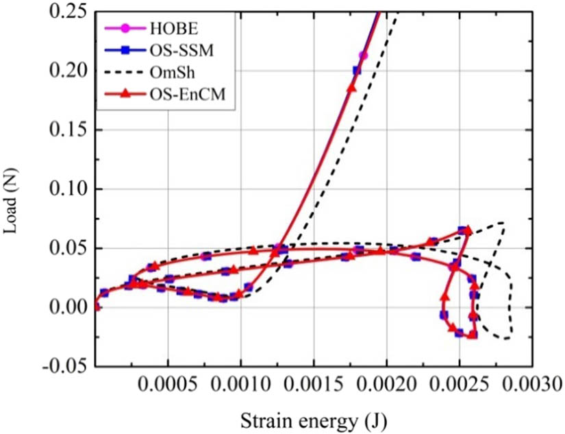
The total number of iterations and the number of load steps utilized to reach the maximum proscribed load when tracing the complete nonlinear equilibrium path for the OmSh, OS-SSM, OS-EnCM, and HOBE are shown in Table 1. The simulated deflection of Lee’s frame can be seen in Figure 3, whereas x-deflection and y-deflection can be seen in Figures 4 and 5, respectively. The variation of strain energy according to the change in applied load is shown in Figure 6. The whole 3D equilibrium path using HOBE can be found in Figure 7. It can be observed that the OmSh slightly overpredicts the limit point postbuckling load as compared to the ANSYS BEAM188 reference solution. The results produced by the OS-SSM, OS-EnCM, and HOBE agree well with the reference solution. The complete snap-back nonlinear postbuckling response of Lee’s frame with pinned–pinned boundary conditions is successfully predicted by ANCF-based approaches. However, it is found that the total number of iterations required to complete the path is minimum for the OmSh and then OS-EnCM. It is slightly higher for the OS-SSM and much higher for the HOBE. It should be further noted that the HOBE required only two iterations per incremental load step to reach the equilibrium state and does not present any convergence-related issues.

Figure 3

Lee’s frame with pinned–pinned boundary conditions and contour represents von Mises stress (Case 1).

Figure 4

Snap-back of Lee’s frame showing x-deflection (Case 1).

Figure 5

Snap-back of Lee’s frame showing y-deflection (Case 1).

Figure 6

Strain energy of snap-back of Lee’s frame (Case 1).

Figure 7

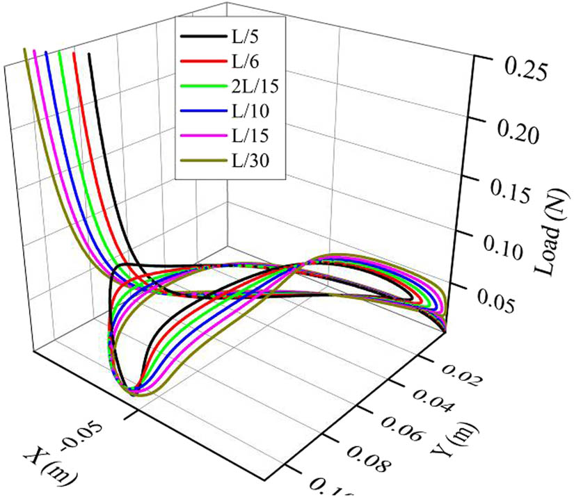
Complete 3D equilibrium path of snap-back of Lee’s frame (Case 1) with varying offset load points.

The buckling analysis based on the energy criterion utilizing the HOBE, OS-EnCM, and OmSh approaches is successfully conducted for Lee’s frame with pinned–pinned boundary conditions. It is found that the OS-SSM failed to converge to the solution. Therefore, it is not included in Table 2. For comparison with the reference solution, 200 ANSYS BEAM188 elements are used to calculate the critical buckling load, and the obtained results are presented in Table 2. It can be seen that the ANCF-based HOBE and OS-EnCM results for the first, second, and third buckling loads are in good agreement with the reference, whereas the OmSh overpredicts the three buckling loads. The three buckling mode shapes simulated using the HOBE are shown in Figure 8.

Figure 8

Buckling mode shapes for Lee’s frame with pinned–pinned BCs (Case 1).

It should be noted that the energy criterion-based buckling analysis is done when the load is applied in the vertically downward direction at the rigid joint of Lee’s frame, not offsetting by L/5, as in the nonlinear postbuckling analysis. Because the concept for using the buckling analysis is to model the perfect initial geometry with loading conditions of the structure without any imperfection, i.e., without any introduction of small perturbation load or eccentric displacement in the form of a small offset. On the contrary, for the nonlinear postbuckling analysis, the nonlinear large deformation analysis is done by allowing the imperfection so that the whole nonlinear equilibrium path can be traced and the limit point postbuckling loads can be found. In further investigation, the HOBE approach is utilized while the offset point of the load is varied to find the lowest limit load, but L/5 is found to give the lowest value. Hence, we can see that the 0.0138 N critical buckling load is less than the 0.018 N limit point postbuckling load given by the L/5 offset. Therefore, the critical buckling load obtained by the energy criterion-based buckling analysis should be used as the maximum allowed load.

5.2 Case 2: Snap-through of Lee’s frame

The whole nonlinear equilibrium path in the form of the snap-through response for Lee’s frame with pinned-fixed boundary conditions is traced. The deflected frame after equal intervals can be seen in Figure 9, while the deflection in the x- and y-axis against load can be observed in Figures 10 and 11, respectively. The variation of strain energy according to the change in applied load is shown in Figure 12. The complete 3D equilibrium path using HOBE can be seen in Figure 13. The numerical results are presented in Table 3. It is observed from the data that the OmSh predicts a slightly higher limit load than the reference ANSYS BEAM188 solution due to the presence of the locking. Whereas the other ANCF-based approaches, i.e., OS-SSM, OS-EnCM, and HOBE, have no considerable difference. The number of load steps and the total number of iterations required to complete the path are highest for the HOBE, high for the OS-SSM, while it is least for the OmSh and OS-EnCM. Additionally, it is important to notice that the OmSh, OS-EnCM, and HOBE only require two iterations per incremental load step to converge to the equilibrium state. The OS-SSM, in this case of snap-through buckling of Lee’s frame, sometimes requires a higher number of iterations than two per incremental load step.

Figure 9

Lee’s frame with pinned-fixed boundary conditions where contour represents von Mises stress (Case 2).

Figure 10

Snap-through of Lee’s frame showing x-deflection (Case 2).

Figure 11

Snap-through of Lee’s frame showing y-deflection (Case 2).

Figure 12

Strain energy graph of snap-through of Lee’s frame (hinged-fixed).

Figure 13

Complete 3D equilibrium path of snap-through of Lee’s frame (Case 2) with varying offset load points.

Similarly, as in the previous case, for the energy criterion-based buckling analysis OS-SSM failed to converge. But, the ANCF-based HOBE, OS-EnCm, and OmSh approaches converged, and the obtained solutions are shown in Table 4. The mode shapes obtained utilizing the HOBE approach are shown in Figure 14. The HOBE and OS-EnCM results for all three critical buckling loads match well with the ANSYS BEAM188 results, whereas, due to the locking phenomenon present in the OmSh element, the predicted critical load is higher.

Figure 14

Buckling mode shapes for Lee’s frame with pinned-fixed BCs (Case 2).

While using the HOBE approach, the offset point of the load is varied in the range of L/5 to L/30, but it was found that the L/5 offset gives the lowest value for the first limit load. After, the energy criterion-based buckling analysis and nonlinear postbuckling analysis results are compared. It is found that the first critical buckling load 0.027 N is higher than the postbuckling limit load 0.018 N, which means that the chance of limit point buckling occurring is higher. Therefore, the limit point postbuckling load should be used as the maximum allowed load.

5.3 Case 3: Lee’s frame with looping phenomenon (fixed–fixed)

The first limit points of the nonlinear equilibrium path of Lee’s frame with fixed–fixed boundary conditions are presented in Table 5. From the comparison of the OmSh, OS-EnCM, OS-SSM, and HOBE results against the ANSYS BEAM188, it can be seen that the OS-SSM failed to complete the whole nonlinear equilibrium path. Lee’s frame deflections are simulated in Figure 15, while the x-deflection and y-deflection can be observed in Figures 16 and 17, respectively. The variation of strain energy according to the change in applied load is shown in Figure 18. The whole nonlinear equilibrium path is shown in Figure 19. The whole nonlinear equilibrium path using HOBE is shown in Figure 16. The HOBE results are produced using the arc-length parameter Δ l = 0.2 , whereas OmSh and OS-EnCM Δ l = 0.1 are used. For OS-SSM arc-length parameter is further lowered to Δ l = 0.05 even then it did not produce the whole path. For the OS-SSM approach, the first limit point is successfully attained, but the postbuckling behavior present in the form of the looping phenomenon is not captured. As in the previous cases, it can be observed that the OmSh slightly overpredicts the limit point postbuckling load. And, the ANCF-based HOBE and OS-EnCM predicted loads are in good agreement with the reference. On the contrary, it should be noted that the HOBE requires only two iterations per incremental load step to converge to the equilibrium state and successfully completes the whole equilibrium path without having any convergence issues.

Figure 15

Lee’s frame with fixed–fixed boundary conditions where contour represents von Mises stress (Case 3).

Figure 16

Lee’s frame with looping phenomenon showing x-deflection (Case 3).

Figure 17

Lee’s frame with looping phenomenon showing y-deflection (Case 3).

Figure 18

Strain energy graph of looping phenomenon of Lee’s frame (Case 3).

Figure 19

Complete 3D equilibrium path of looping phenomenon of Lee’s frame (Case 3) with varying offset load points.

During the energy criterion-based buckling analysis, for Lee’s frame with fixed–fixed boundary conditions, the ANCF-based OS-SSM element failed to converge. On the other hand, the ANCF-based OmSh, OS-EnCM, and HOBE give a result that agrees well with the ANSYS BEAM188-produced solution, as shown in Table 6. It can be seen that OmSh overpredicts the critical buckling loads. Hence, the three critical buckling loads and corresponding mode shapes are successfully extracted using HOBE. Three mode shapes obtained using the HOBE approach can be seen in Figure 20. While investigating the various offset load points, using the HOBE approach, it is found that the L/6 offset point gives the lowest first limit point load as 0.03395 N. As the lowest critical buckling load is 0.028 N which is less than the postbuckling limit load of the concern, the critical buckling load based on energy criterion should be used as the maximum allowed load.

Figure 20

Buckling mode shapes for Lee’s frame with fixed–fixed BCs (Case 3).

5.4 Case 4: Lee’s frame with looping phenomenon (fixed-pinned)

During the nonlinear postbuckling analysis, the looping behavior of Lee’s frame with fixed-pinned boundary conditions is simulated, and numerical results are presented in Table 7. The deflected Lee’s frame under loading is shown in Figure 21, whereas deflection graphs in the x- and y-axis can be observed in Figures 22 and 23, respectively. The variation of strain energy according to the change in applied load is shown in Figure 24. The complete 3D nonlinear equilibrium path obtained using HOBE is shown in Figure 25. The HOBE results are produced using the arc-length parameter as Δ l = 0.2 , whereas for OmSh and OS-EnCM Δ l = 0.1 is used. For, the OS-SSM approach, arc-length parameter was further lowered to Δ l = 0.05 in order to produce the whole path and it successfully traced the whole path. Nonetheless, the first limit points for the OmSh, OS-SSM, OS-EnCM, and HOBE are obtained and compared against the ANSYS BEAM188 reference solution. As, in the previous three cases, the OmSh approach slightly overpredicts the limit load due to the presence of locking. OS-SSM, OS-EnCM, and HOBE are found to be in good agreement with the reference ANSYS BEAM188 solution. On the contrary, it should be noted that the HOBE and OS-EnCM needed only two iterations per incremental load step while tracing the whole complex looping path and successfully completed it without presenting any convergence related issues.

Figure 21

Lee’s frame with fixed-pinned boundary conditions where contour represents von Mises stress (Case 4).

Figure 22

Lee’s frame with looping phenomenon showing x-deflection (Case 4).

Figure 23

Lee’s frame with looping phenomenon showing y-deflection (Case 4).

Figure 24

Strain energy graph of looping phenomenon of Lee’s frame (Case 4).

Figure 25

Complete 3D equilibrium path of looping phenomenon of Lee’s frame (Case 4) with varying offset load points.

In this case, the energy criterion-based buckling analysis for the OS-SSM element failed to converge. But, the ANCF-based HOBE, OS-EnCM, and OmSh approaches converged to the solution which is shown in Table 8. The result produced by the HOBE and OS-EnCM are found to be in good agreement with the ANSYS BEAM188 result for the three critical buckling loads. The three mode shapes using the HOBE approach are shown in Figure 26. Upon varying the offset load points and tracing the whole equilibrium path using the HOBE approach, it is found that the L/15 gives the lowest first limit load value as 0.04015 N. It is observed that the postbuckling limit load of concern is many times higher than the lowest critical buckling load of 0.014 N. Therefore, the maximum allowed load should not exceed the critical buckling load obtained by the energy criterion.

Figure 26

Buckling mode shapes for Lee’s frame with fixed-pinned BCs (Case 4).

5.5 Case 5: Roorda’s frame

As it can be seen from the previous numerical problems, the ANCF-based HOBE approach is the best approach among the studied ANCF approaches for the nonlinear frame analysis. For further verification and validation, comparison with the experimental result is a must. Hence, the L-frame from Roorda’s experiment is studied here.

Koiter, in his landmark thesis, applied the perturbation-based numerical technique to estimate the buckling load of the L-frame, which is given by the formula P / P c r = 1 − 0.3805 θ . And, the buckling load is given by P c r = 1.407 π 2 E I / L 2 . Rizzi et al. used a more sophisticated analytical approach incorporating up to fourth-order terms; the solution produced by them is P / P c r = 1 − 0.3805 θ + 0.4638 θ 2 . Further, Galvão et al. utilized an efficient nonlinear finite element formulation for the analysis of planar elastic frames together with a nonlinear solution methodology. In Figures 27, amd 28 and data from Galvão’s publication are used as a reference, which already contains Rizzi et al., Koiter and Roorda results [43]. These reference results are then compared with 60 elements using the ANCF-based HOBE approach.

Figure 27

Postbuckling solution for the Roorda’s frame.

Figure 28

Comparison between ANCF based HOBE, Roorda’s experiment, Koiter’s perturbation technique, Rizzi’s analytical solution and Galvão’s nonlinear solution.

Rizzi et al. conducted a thorough parametric analysis of the two-bar frame problem by using the modified potential energy approach. This analysis was profound yet simple, allowing us to incorporate the fourth-order terms in the analytical solution. But, from Figures 27 and 28, when the analytical results of Rizzi, Roorda’s experimental, and Koiter’s perturbation approach are compared, it can be seen that Galvão’s nonlinear solution and ANCF HOBE solution are much better.

References

[1] Shabana AA. Definition of the slopes and the finite element absolute nodal coordinate formulation. Multibody Syst Dyn. 1997;1(3):339–48.10.1023/A:1009740800463Search in Google Scholar
[2] Shabana AA. Definition of ANCF finite elements. J Comput Nonlinear Dyn. 2015;10(5):054506(1–5).10.1115/1.4030369Search in Google Scholar
[3] Shabana AA. Computational continuum mechanics. 3rd ed. Hoboken (NJ), USA: John Wiley & Sons Ltd; 2018. p. 363.10.1002/9781119293248Search in Google Scholar
[4] Shabana AA. ANCF tire assembly model for multibody system applications. J Comput Nonlinear Dyn. 2015;10(2):024504(1–4).10.1115/1.4028479Search in Google Scholar
[5] Yu Z, Liu Y, Tinsley B, Shabana AA. Integration of geometry and analysis for vehicle system applications: Continuum-based leaf spring and tire assembly. J Comput Nonlinear Dyn. 2016;11(3):031011(1–11).10.1115/1.4031151Search in Google Scholar
[6] Wang T, Tinsley B, Patel MD, Shabana AA. Nonlinear dynamic analysis of parabolic leaf springs using ANCF geometry and data acquisition. Nonlinear Dyn. 2018;93:2487–515. 10.1007/s11071-018-4338-3.Search in Google Scholar
[7] Cui Y, Lan P, Zhou H, Yu Z. The rigid-flexible-thermal coupled analysis for spacecraft carrying large-aperture paraboloid antenna. J Comput Nonlinear Dyn. 2020;15(3):031003(1–13).10.1115/1.4045890Search in Google Scholar
[8] Liu C, Tian Q, Yan D, Hu H. Dynamic analysis of membrane systems undergoing overall motions, large deformations and wrinkles via thin shell elements of ANCF. Comput Methods Appl Mech Eng. 2013;258:81–95. 10.1016/j.cma.2013.02.006.Search in Google Scholar
[9] Li K, Tian Q, Shi J, Liu D. Assembly dynamics of a large space modular satellite antenna. Mech Mach Theory. 2019;142(103601):1–18.10.1016/j.mechmachtheory.2019.103601Search in Google Scholar
[10] Shabana AA, Eldeeb AE. Motion and shape control of soft robots and materials. Nonlinear Dyn. 2021;104:165–89. 10.1007/s11071-021-06272-y.Search in Google Scholar
[11] Huang X, Zou J, Gu G. Kinematic modeling and control of variable curvature soft continuum robots. IEEE/ASME Trans. Mechatronics. 2021;26:1–11.10.1109/TMECH.2021.3055339Search in Google Scholar
[12] Hu H, Tian Q, Liu C. Computational dynamics of soft machines. Acta Mech Sin. 2017;33:516–28.10.1007/s10409-017-0660-0Search in Google Scholar
[13] Yoo W-S, Dmitrochenko O, Pogorelov DY. Review of finite elements using absolute nodal coordinates for large-deformation problems and matching physical experiments. ASME 2005 International design Engineering Technical Conferences and Computers and Information in Engineering Conference. 2005 Sep 24–28; Long Beach (CA), USA. ASME, 2005.10.1115/DETC2005-84720Search in Google Scholar
[14] Gerstmayr J, Hiroyuki S, Aki M. Review on the absolute nodal coordinate formulation for large deformation analysis of multibody systems. J Comput Nonlinear Dyn. 2013;8(3):031016(1–12).10.1115/1.4023487Search in Google Scholar
[15] Dmitrochenko O, Mikkola A. Digital nomenclature code for topology and kinematics of finite elements based on the absolute nodal co-ordinate formulation. Proc Inst Mech Eng Part K J Multi-body Dyn. 2011;225(1):34–51.10.1177/2041306810392115Search in Google Scholar
[16] Luo K, Liu C, Tian Q, Hu H. Nonlinear static and dynamic analysis of hyper-elastic thin shells via the absolute nodal coordinate formulation. Nonlinear Dyn. 2016;85:949–71.10.1007/s11071-016-2735-zSearch in Google Scholar
[17] Li J, Liu C, Hu H, Zhang S. Analysis of elasto-plastic thin-shell structures using layered plastic modeling and absolute nodal coordinate formulation. Nonlinear Dyn. 2021;105:2899–920.10.1007/s11071-021-06766-9Search in Google Scholar
[18] Nachbagauer K, Gerstmayr J. Structural and continuum mechanics approaches for a 3D shear deformable ANCF beam finite element: Application to buckling and nonlinear dynamic examples. J Comput Nonlinear Dyn. 2013;9(1):1–8. 10.1115/1.4025282.Search in Google Scholar
[19] Shaukat AR, Lan P, Wang J, Wang T. In-plane nonlinear postbuckling analysis of circular arches using absolute nodal coordinate formulation with arc-length method. Proc Inst Mech Eng Part K J Multi-body Dyn. 2021 Sep;235(3):297–311.10.1177/1464419320971412Search in Google Scholar
[20] Wang J, Wang T. Buckling analysis of beam structure with absolute nodal coordinate formulation. Proc Inst Mech Eng Part C J Mech Eng Sci. 2021 May;235(9):1585–92.10.1177/0954406220947117Search in Google Scholar
[21] Reis PM. A perspective on the revival of structural (In)stability with novel opportunities for function: From Buckliphobia to Buckliphilia. J Appl Mech. 2016;82(11):1–4.10.1115/1.4031456Search in Google Scholar
[22] Cox BS, Groh RMJ, Avitabile D, Pirrera A. Exploring the design space of nonlinear shallow arches with generalised path-following. Finite Elem Anal Des. 2018;143:1–10.10.1016/j.finel.2018.01.004Search in Google Scholar
[23] Hunt G, Champneys A, Dodwell T, Groh R, Neville R, Pirrera A, et al. Happy Catastrophe: recent progress in analysis and exploitation of elastic instability. Front Appl Math Stat. 2019;5:34.10.3389/fams.2019.00034Search in Google Scholar
[24] Pal A, Restrepo V, Goswami D, Martinez RV. Exploiting mechanical instabilities in soft robotics: Control, sensing, and actuation. Adv Mater. 2021;33(19):1–18.10.1002/adma.202006939Search in Google Scholar PubMed
[25] Shabana AA, Gantoi FM, Brown MA. Integration of finite element and multibody system algorithms for the analysis of human body motion. Procedia IUTAM. 2011;2:233–40.10.1016/j.piutam.2011.04.022Search in Google Scholar
[26] Orzechowski G, Fraczek J. Nearly incompressible nonlinear material models in the large deformation analysis of beams using ANCF. Nonlinear Dyn. 2015;82:451–64.10.1007/s11071-015-2167-1Search in Google Scholar
[27] Maqueda LG, Mohamed AA, Shabana AA. Use of General Nonlinear Material Models in Beam Problems: Application to Belts. J Comput Nonlinear Dyn. 2010;5:021003.10.1115/1.4000795Search in Google Scholar
[28] Pil Jung S, Won Park T, Sun Chung W. Dynamic analysis of rubber-like material using absolute nodal coordinate formulation based on the non-linear constitutive law. Nonlinear Dyn. 2011;63:149–57.10.1007/s11071-010-9792-5Search in Google Scholar
[29] Karl-Eugen K. The history of the theory of structures – from arch analysis to computational mechanics. Berlin, Germany: Ernst & Sohn Verlag; 2008.Search in Google Scholar
[30] Timoshenko SP, Gere JM. Theory of elastic stability. 17th ed. London, UK: McGraw; 1963. p. 541Search in Google Scholar
[31] Koiter WT. Post-Buckling Analysis of a Simple Two-Bar Frame. Almquist and Wiksell Stockholm, Sweden: 1967. p. 337–54.Search in Google Scholar
[32] Roorda J, Chilver AH. Frame buckling: An illustration of the perturbation technique. Int J Non Linear Mech. 1970;5(2):235–46.10.1016/0020-7462(70)90021-1Search in Google Scholar
[33] Lee S-L, Manuel FS, Rossow EC. Large deflections and stability of elastic frame. J Eng Mech Div. 1968;94(2):521–48.10.1061/JMCEA3.0000966Search in Google Scholar
[34] Akkoush EA, Toridis TG, Khozeimeh K, Huang HK. Bifurcation, pre- and post-buckling analysis of frame structures. Comput Struct. 1978;8(6):667–78.10.1016/0045-7949(78)90143-8Search in Google Scholar
[35] Simitses GJ, Giri J, Kounadis ANE. Nonlinear analysis of portal frames. Int J Numer Methods Eng. 1981;17:123–32.10.1002/nme.1620170110Search in Google Scholar
[36] Simitses GJ, Giri J. Asymmetrically loaded portal frames. Comput Struct. 1984;19(4):555–8.10.1016/0045-7949(84)90102-0Search in Google Scholar
[37] Kounadis AN, Giri J, Simitses GJ. Nonlinear stability analysis of an eccentrically loaded two-bar frame. J Appl Mech Trans ASME. 1977;44(4):701–6.10.1115/1.3424160Search in Google Scholar
[38] Pignataro M, Rizzi N. The effect of multiple buckling modes on the postbuckling behavior of plane elastic frames. Part I. Symmetric Frames. J Struct Mech. 1982;10(4):437–58.10.1080/03601218208907423Search in Google Scholar
[39] Rizzi N, Pignataro M. The effect of multiple buckling modes on the postbuckling behavior of plane elastic frames. Part II. Symmetric frames. J Struct Mech. 1982;10(4):459–74.10.1080/03601218208907424Search in Google Scholar
[40] Pignataro M, Rizzi N. On the interaction between local and overall buckling of an asymmetric portal frame. Meccanica. 1983;18(2):92–6.10.1007/BF02128349Search in Google Scholar
[41] Pacoste C, Eriksson A. Beam elements in instability problems. Comput Methods Appl Mech Eng. 1997;144(1–2):163–97.10.1016/S0045-7825(96)01165-6Search in Google Scholar
[42] Waszczyszyn Z, Janus-Michalska M. Numerical approach to the “exact” finite element analysis of in-plane finite displacements of framed structures. Comput Struct. 1998;69(4):525–35.10.1016/S0045-7949(98)00115-1Search in Google Scholar
[43] Galvão AS, Gonçalves PB, Silveira RAM. Post-buckling behavior and imperfection sensitivity of L-frames. Int J Struct Stab Dyn. 2005;5(1):19–35.10.1142/S021945540500143XSearch in Google Scholar
[44] Basaglia C, Camotim D, Silvestre N. Post-buckling analysis of thin-walled steel frames using generalised beam theory (GBT). Thin-Walled Struct. 2013;62:229–42. 10.1016/j.tws.2012.07.003.Search in Google Scholar
[45] Yeong-Bin Y, Shyh-Rong K. Theory and analysis of nonlinear framed structures. 1st ed. Upper Saddle River (NJ), USA: Prentice Hall; 1994. p. 569.Search in Google Scholar
[46] Yeong-Bin Y, Anquan C, Song H. Research on nonlinear, postbuckling and elasto-plastic analyses of framed structures and curved beams. Meccanica. 2020;56:1587–612. 10.1007/s11012-020-01182-6.Search in Google Scholar
[47] Omar MA, Shabana AA. A two-dimensional shear deformable beam for large rotation and deformation problems. J Sound Vib. 2001;243(3):565–76.10.1006/jsvi.2000.3416Search in Google Scholar
[48] Patel M, Shabana AA. Locking alleviation in the large displacement analysis of beam elements: the strain split method. Acta Mech. 2018;229:2923–46.10.1007/s00707-018-2131-5Search in Google Scholar
[49] Gerstmayr J, Matikainen MK, Mikkola AM. A geometrically exact beam element based on the absolute nodal coordinate formulation. Multibody Syst Dyn. 2008;20(4):359–84.10.1007/s11044-008-9125-3Search in Google Scholar
[50] Shen Z, Li P, Liu C, Hu G. A finite element beam model including cross-section distortion in the absolute nodal coordinate formulation. Nonlinear Dyn. 2014;77:1019–33.10.1007/s11071-014-1360-ySearch in Google Scholar
[51] Orzechowski G, Shabana AA. Analysis of warping deformation modes using higher order ANCF beam element. J Sound Vib. 2016;363:428–45.10.1016/j.jsv.2015.10.013Search in Google Scholar
[52] Shabana AA, Mikkola AM. Use of the finite element absolute nodal coordinate formulation in modeling slope discontinuity. J Mech Des Trans ASME. 2003;125(2):342–50.10.1115/1.1564569Search in Google Scholar
[53] Wempner GA. Discrete approximations related to nonlinear theories of solids. Int J Solids Struct. 1971;7(11):1581–99.10.1016/0020-7683(71)90038-2Search in Google Scholar
[54] Riks E. An incremental approach to the solution of snapping and buckling problems. Int J Solids Struct. 1978;15(7):529–51.10.1016/0020-7683(79)90081-7Search in Google Scholar
[55] Crisfield MA. A fast incremental/iterative solution procedure that handles “Snap-through”. Comput Struct. 1981;13(1–3):55–62.10.1016/0045-7949(81)90108-5Search in Google Scholar
[56] de Borst R, Crisfield MA, Remmers JJC, Verhoosel CV. Non-linear finite element analysis of solids and structures. Chichester, UK: John Wiley & Sons; 2012.10.1002/9781118375938Search in Google Scholar
[57] Simitses G, Hodges DH. Fundamentals of structural stability. 1st ed. Oxford, UK: Butterworth-Heinemann; 2006.Search in Google Scholar
© 2023 the author(s), published by De Gruyter
This work is licensed under the Creative Commons Attribution 4.0 International License.
Articles in the same Issue
- Research Articles
- Investigation of differential shrinkage stresses in a revolution shell structure due to the evolving parameters of concrete
- Multiphysics analysis for fluid–structure interaction of blood biological flow inside three-dimensional artery
- MD-based study on the deformation process of engineered Ni–Al core–shell nanowires: Toward an understanding underlying deformation mechanisms
- Experimental measurement and numerical predictions of thickness variation and transverse stresses in a concrete ring
- Studying the effect of embedded length strength of concrete and diameter of anchor on shear performance between old and new concrete
- Evaluation of static responses for layered composite arches
- Nonlocal state-space strain gradient wave propagation of magneto thermo piezoelectric functionally graded nanobeam
- Numerical study of the FRP-concrete bond behavior under thermal variations
- Parametric study of retrofitted reinforced concrete columns with steel cages and predicting load distribution and compressive stress in columns using machine learning algorithms
- Application of soft computing in estimating primary crack spacing of reinforced concrete structures
- Identification of crack location in metallic biomaterial cantilever beam subjected to moving load base on central difference approximation
- Numerical investigations of two vibrating cylinders in uniform flow using overset mesh
- Performance analysis on the structure of the bracket mounting for hybrid converter kit: Finite-element approach
- A new finite-element procedure for vibration analysis of FGP sandwich plates resting on Kerr foundation
- Strength analysis of marine biaxial warp-knitted glass fabrics as composite laminations for ship material
- Analysis of a thick cylindrical FGM pressure vessel with variable parameters using thermoelasticity
- Structural function analysis of shear walls in sustainable assembled buildings under finite element model