Reliability-based assessment of ship hull girder ultimate strength
-
Ristiyanto Adiputra
 ,
Takao Yoshikawa
,
Takao Yoshikawa

Abstract
A reliability-based approach is presented to investigate the effects of structural and load uncertainties on the reliability estimation of ship hull girders. Structural uncertainties included randomness in material properties, geometric properties, initial geometric imperfections, and corrosion behavior. Load uncertainties included statistical uncertainties, model uncertainties, environmental uncertainties, and uncertainties related to nonlinearity. The hull girder ultimate strength was calculated using Smith’s method, and the probabilistic density function was evaluated by employing Monte Carlo simulations. In the load estimation, the still water bending moment and wave-induced bending moment were calculated using a simplified formula of the International Association of Classification Societies-Common Structural Rules code and then modified with load parameters. The reliability index was estimated using a first-order reliability method considering the operating time, the duration of the ship in the alternate hold loading condition, and the severity of the corrosion rate. As a result, sagging conditions dominated the collapse mode. The reliability indexes were obtained for the observed cases, and the viability of the ship was assessed accordingly.
Nomenclature
List of symbols
-
-
net sectional area, in cm2, of attached plating
-
-
effective area of the plate, in cm2
-
-
net sectional area, in cm2, of stiffener
-
-
ordinary stiffener spacing, in m
-
-
breadth of the ship, in m
-
-
maximum amplitude of initial imperfection for column and torsional buckling mode
-
-
distance of the transverse stiffener, in m
-
-
effective width of the stiffener, in mm
-
-
correction factor due to randomness in yield stress
-
-
correction factor for yield stress reduction due to initial imperfection
-
-
block coefficient of the ship
-
-
cumulative distribution of peak value of WIBM
-
-
cumulative probability function of SWBM in one voyage
-
-
cumulative probability function of WIBM in the given period
-
-
probability density function of SWBM in one voyage
-
-
net web height, in mm
-
-
effective height of the stiffener, in mm
-
-
length of the ship, in m
-
-
length of the FEM model of stiffened panel
-
-
bending moment in still water condition (SWBM)
-
-
the characteristic value of SWBM
-
-
total vertical bending moment
-
-
wave-induced bending moment (WIBM)
-
-
the characteristic value of WIBM
-
-
number of wave cycles encountered by the ship in the given period
-
-
number of voyages in a particular period
-
-
minimum yield stress, in N/mm2, of the plate
-
-
minimum yield stress, in N/mm2, of the stiffener
-
-
thickness of the flange, in mm
-
-
thickness of base plate, in mm
-
-
thickness of the web, in mm
-
-
maximum amplitude of initial imperfection for local buckling mode
-
-
model uncertainty in SWBM estimation
-
-
statistical uncertainty in SWBM estimation
-
-
environmental uncertainty in WIBM estimation
-
-
model uncertainty in WIBM estimation
-
-
uncertainty due to nonlinearity in WIBM estimation
-
-
statistical uncertainty in WIBM estimation
List of Greek symbols
-
-
reliability index
-
-
effective plate slenderness
-
-
shape parameter of the extreme value distribution of SWBM
-
-
scale parameter of the extreme value distribution of SWBM
-
-
scale parameter of the Weibull distribution of WIBM in each cycle
-
-
shape parameter of the Weibull distribution of WIBM in each cycle
-
-
mean value of statistical uncertainty of SWBM
-
-
mean value of statistical uncertainty of WIBM
-
-
standard deviation of statistical uncertainty of SWBM
-
-
standard deviation of statistical uncertainty of WIBM
-
-
critical stress in N/mm2 for each respective buckling mode
-
-
buckling stress of attached plate in N/mm2
-
-
ultimate strength of stiffened panel under column buckling
-
-
ultimate strength of stiffened panel under torsional buckling
-
-
ultimate strength of stiffened panel made of flanged profiles under web local buckling
-
-
ultimate strength of stiffened panel made of flat bars under web local buckling
-
-
ultimate strength of plate buckling
-
-
edge function
-
-
load combination factor
List of abbreviations
- CSR
-
Common Structural Rules
- HGUS
-
hull girder ultimate strength
- IACS
-
International Association of Classification Societies
- ISSC
-
International Ship and Offshore Structures Congress
- SWBM
-
still water bending moment
- WIBM
-
wave-induced bending moment
1 Introduction
Sea transport is the most efficient way to deliver cargo worldwide, with bulk carriers transporting over 30% of ocean cargo globally [1]. Despite this, a study on the safety assessment of bulk carriers [2] reported that from 1975 to 1996, there were more than 500 casualties, where the first event was a structural failure. For additional consideration, Lloyd’s records indicated that more than 500 bulk carriers were involved in accidents between 1980 and 2010 [3]. In the recent record by the International Association of Dry Cargo Shipowners, between 2009 and 2018, 48 bulk carriers carrying over 10,000 dead weight tonnage suffered casualties that caused over 100 deaths [4]. Although bulk carrier safety has progressed in recent decades, the above data suggest that a more detailed and advanced study should be conducted to ensure that the structural capabilities of the ship can withstand the loads under various conditions.
Conventionally, the ship is considered safe when the hull girder ultimate strength (HGUS) exceeds its total bending moment by a certain margin. However, in reality, the parameters of HGUS and load calculation are random [5]. So, instead of a deterministic value, the value of HGUS and total load naturally follow a type of distribution. Failure and fatality may happen when the extreme minimum condition of HGUS meets the severe maximum condition of the total bending moment. Therefore, the crucial parameter of HGUS analysis is not only the mean value but also the standard distribution of the HGUS and total bending moment, where a significant standard deviation indicates an increase in the probability of failure.
Since the early introduction of the reliability method by Mansour [6], substantial and significant improvements have been made in the past decades, taking into account the inclusion of various uncertainties in the strength [7,8,9,10,11], loads [1,12,13,14], and methods [15,16]. Concerning the reliability assessment of bulk carriers, Guedes Soares and Teixeira [17] analyzed the feasibility of converting a single-hull bulk carrier to a double-hull structure. The analysis was focused on the effect of double-hull installation on the reliability index. The effect of corrosion had been considered, yet its corrosion rate was assumed to be constant for particular stiffened elements. Considering the importance of the alternate hold loading (AHL) condition, Shu and Moan calculated the reliability index of bulk carriers focusing on the hogging and AHL conditions but without considering the effects of corrosion [1]. Vhanmane and Bhattacharya included the effects of initial geometric imperfection in the HGUS analysis [18], with the amplitude of initial geometric imperfection introduced based on assumptions.
Efforts have been made to determine the statistical parameters of uncertainties in HGUS and load calculations based on actual data. For example, the proposed data in ref. [19] show the randomness of the initial geometric imperfection, and the data in ref. [20] predict the corrosion wastage based on the actual inspection. Despite the significant effects of these uncertainties on the HGUS, the Smith’s method commonly used to calculate the HGUS does not explicitly account for corrosion and initial geometric imperfection in the load-shortening equations of the stiffened panels [21,22,23].
Corrosion can be accounted for simply by justifying the net thickness of the plate as the gross thickness minus the corrosion wastage for specific years of service. However, introducing the initial geometric imperfection into the hull girder is time-consuming and requires high computational resources. Moreover, in the reliability analysis, the HGUS must be evaluated for hundreds of data sets generated from the probabilistic parameters of each uncertainty by Monte Carlo simulation [24,25,26].
To simplify the calculation, in this work, the effect of the initial geometric imperfection on the ultimate strength of all stiffened panels is calculated and then transferred to the HGUS calculation in the form of a reduction in yield stress. In other words, the effect of the initial geometric imperfection corresponds to the reduction in yield strength and the effect of corrosion behavior corresponds to the decrease in thickness of the stiffened panel. As a reference, the ISSC-2000 Capesize bulk carrier [27] was used. The procedure to model its stiffened panels in the finite element method was adapted from [28,29], with the continuous boundary conditions following [29,30].
In the case of load calculation, [1,31,32,33] had stated the uncertainties in a detailed manner, including statistical uncertainty, model uncertainty, environmental uncertainty, and uncertainty due to nonlinearity, where the International Association of Classification Societies-Common Structural Rules (IACS-CSR) code [21] was used to initially calculate the characteristic values of both the still water bending moment (SWBM) and the wave-induced bending moment (WIBM). To bear the undesirable condition and obtain a more rational design bending moment and a suitable load density function [22,34,35] adjusted the analysis to severe environmental and loading conditions and [1,36] introduced a proper load combination factor.
In the reliability assessment, the more uncertainties are considered more accurate the analysis becomes. However, accounting for all uncertainties can be time-consuming and inefficient. It is necessary to focus on the uncertainties that may have more significant impacts on the computational results as conducted in this study. In addition, to obtain a more accurate analysis, this study evaluates the capability of hull girders to withstand the applied bending moment by considering the uncertainties in both HGUS and load calculations, in which the use of randomness parameters is based on actual data [19,20]. The reliability index is estimated using a first-order reliability method (FORM) [37,38,39], and the viability of the ship is carefully evaluated based on the target reliability index [38,40].
2 Analysis environment
2.1 Reference model
The bulk carrier used for this present study was the ISSC-2000 Capesize bulk carrier [27]. The cross-section of its hull girder is shown in Figure 1. This type of bulk carrier has longitudinal strengthening except for the side shell between the top side tank and the bilge hopper tank, which is transversely stiffened [1].
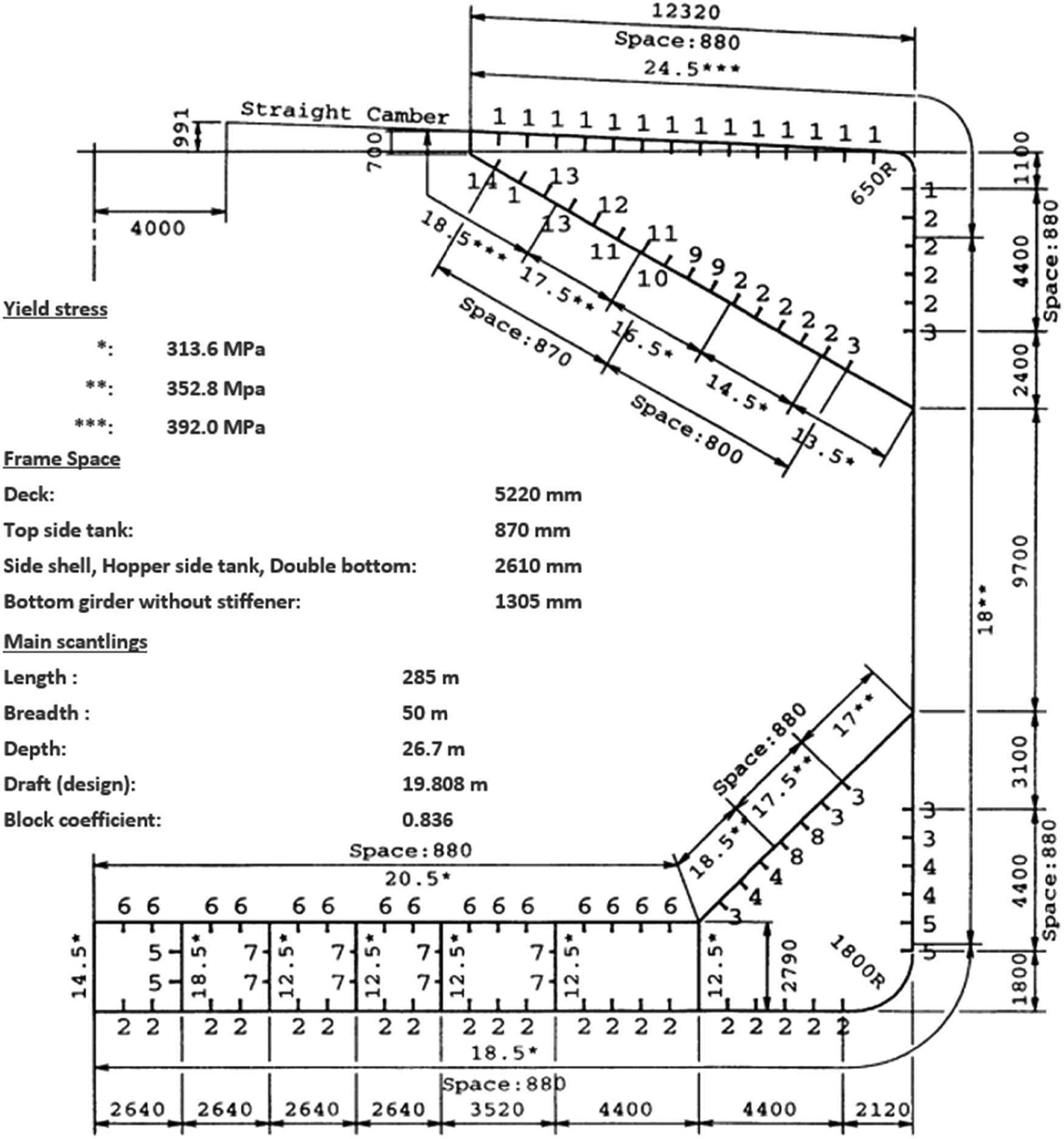
Hull girder cross-section of the ISSC-2000 bulk carrier.
2.2 Case configuration
Mainly, the loading conditions of the bulk carriers are homogenous hold loading, AHL conditions, and cargo in two or more adjoining holds [21]. Among those loading conditions, the alternate loading condition is the most critical for the safe design of bulk carriers [1]. The alternate loading condition is applied for carrying high-density cargos in odd-numbered cargo holds, as shown in Figure 2. When the cargo is distributed in odd-numbered cargo holds, it gives double the cargo weight per hold of homogenous loading, precipitating the maximum shearing force of the hull girder caused by the opposite-acting vertical force of the hull/cargo weight vs buoyancy.
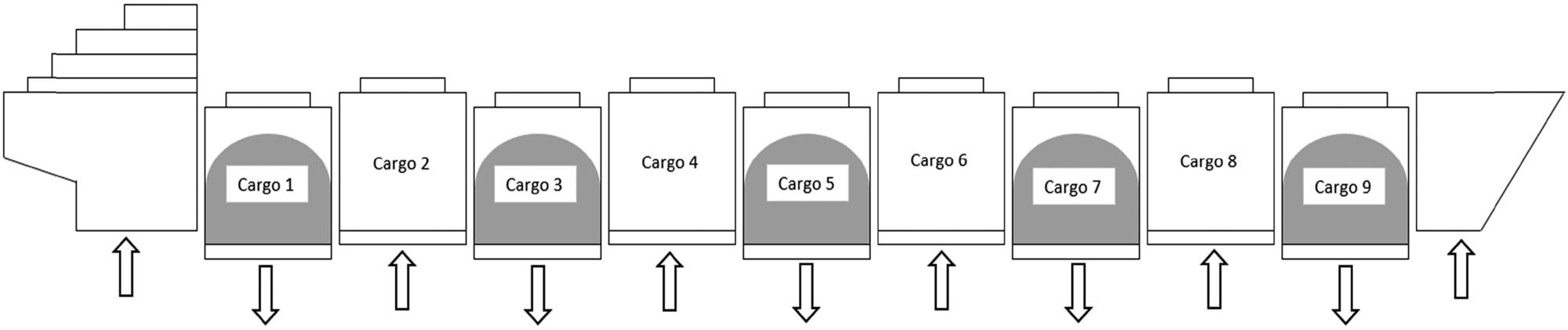
Cargo placement and shearing force direction in AHL condition.
The bulk carrier was assumed to be operated by crossing the North Atlantic and spending 23.5 days finishing 1 voyage [1]. Sea areas in the North Atlantic given by global wave statistics were used to evaluate the WIBM during operation [22], covering world sea areas 8, 9, 11, 15, 16, and 17, as shown in Figure 3 [34].
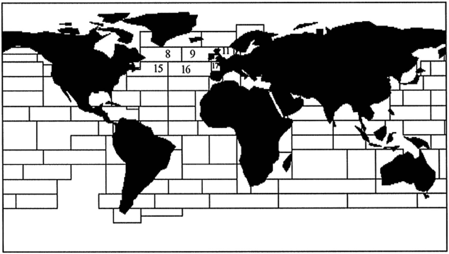
North Atlantic wave scatter data.
When conducting time-dependent reliability analysis, the case configuration was built from two parameters. The first was the duration of the operation, and the second was the duration of the ship spending in AHL condition. The ship operation duration was divided into short-term (1 voyage and 1 year) analysis and long-term (5–25 years with 5 years increments) analysis. The AHL condition was focused on two assumptions. First, the ship was assumed to be in AHL condition for 50% of voyages, and second, the ship was assumed to be in AHL condition for 20% of voyages. The first assumption was that the ship only had one port for unloading at its final destination. The second was to cover the possibility of the ship having two ports for unloading. From the loading port to the first unloading port, the ship was in homogenous loading condition. From the first unloading port to the last unloading port, indicating 20% of the voyage, the ship was in AHL condition. The duration of the ship in the AHL condition affects the number of waves encountered by the ship during operation and then influences the statistical uncertainty of the WIBM. The case configuration is shown in Table 1 and analyzed in both sagging and hogging conditions.
Case configuration
| Case No. | Duration of voyage | AHL duration (%) |
|---|---|---|
| 1 | 1 voyage | 20 |
| 2 | 1 voyage | 50 |
| 3 | 1 year | 20 |
| 4 | 1 year | 50 |
| 5 | 5 years | 20 |
| 6 | 5 years | 50 |
| 7 | 10 years | 20 |
| 8 | 10 years | 50 |
| 9 | 15 years | 20 |
| 10 | 15 years | 50 |
| 11 | 20 years | 20 |
| 12 | 20 years | 50 |
| 13 | 25 years | 20 |
| 14 | 25 years | 50 |
3 Probability study on HGUS
3.1 Incremental-iterative method (Smith’s method)
In Smith’s method, the ultimate strength of the hull girder is calculated at the transverse sections between adjacent transverse webs. A hull girder cross-section is first divided into a set of independent elements. In each incremental step, the incremental curvature is imposed, and the bending moment is generated. Curvature increments correspond to rotation angles of the transverse section of hull girders around their horizontal neutral axis. Then, the corresponding strain and stress are calculated for each element. This procedure is repeated for every step with an updated neutral axis by establishing force equilibrium over the whole transverse section. The corresponding moment is calculated by summing the contributions of all elements. Finally, the maximum HGUS is obtained from the peak value of the curve plotting the vertical bending moment vs the curvature [28]. In the hogging condition, the structural elements above the neutral axis are lengthened while the elements below the neutral axis are shortened, and vice-versa in the sagging condition.
In order to calculate the HGUS, the hull girder cross-section is divided into particular members, where each member contributes to the hull girder strength. The structural members are categorized into stiffener elements, stiffened plate elements, and hard corner elements. The details on this structural element classification and the formulations describing the load-shortening curve for each failure mode of the structural elements are referred to in [21] as listed in Eqs. (1)–(5).
Eq. (1) calculates the stiffener element’s load shortening curve in the column buckling mode, Eq. (2) in the torsional buckling mode, and Eqs. (3) and (4) in the web local buckling mode for flanged profiles and flat bars. These three load-shortening curves are computed for each stiffener element. The maximum stress values for the various failure modes are compared, and the ultimate strength of the stiffener element is determined as the minimum value. In the case of a stiffened plate element, the plate buckling mode of Eq. (5) is used. More in-depth explanations can be found in the IACS-CSR code [21].
Considering its stochastic behavior, the yield stress input data for
3.2 Uncertainties in HGUS
3.2.1 Material and geometric properties
The uncertainties parameter in geometric properties was adopted from [8] as listed in Table 2. Taking into account the quality of the fabrication process and the permissible tolerance, the coefficient of variance for geometric properties was varied between 0.02 and 0.05 and defined following normal distributions.
Randomness in material scantlings
| Variable | Type of distribution | Parameter 1 | Parameter 2 |
|---|---|---|---|
| t p (mm) | Normal | Mean value = Design value | COV = 0.05 |
| t w (mm) | COV = 0.05 | ||
| d w (mm) | COV = 0.02 | ||
| t f (mm) | COV = 0.05 | ||
| b f (mm) | COV = 0.02 |
The stochastic parameter for Young’s modulus was referred from [8] as log–normal distribution with coefficient of variation (COV) of 10% and a bias of 1.00. For randomness in yield strength, which is defined as
Probabilistic parameters of yield strength distribution
| Type of distribution | Design value | Mean value | COV |
|---|---|---|---|
| Log–normal distribution | 313.6 | 348 | 0.06 |
| 352.8 | 390 | 0.06 | |
| 392 | 434 | 0.06 |
3.2.2 Initial geometric imperfection
The proposed scatter data of initial geometric imperfection in ref. [19] was adapted as shown in Figure 4.
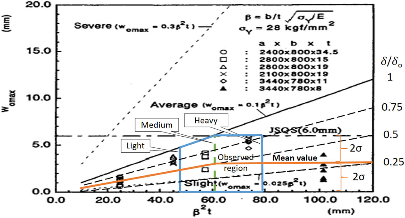
Analyzed scatter data of initial imperfection.
The maximum amplitude of the initial geometric imperfection was calculated as follows:
The maximum amplitude of initial geometric imperfection was defined as a function of the slenderness of plating, calculated as
As stated in Eq. (6), the effect of initial geometric imperfection on the ultimate strength of a hull girder was imposed in terms of yield strength reduction of the respective elements. For this purpose, finite element method (FEM) was first employed to determine the effect of initial geometric imperfection on stiffener elements. However, using FEM to analyze all sizes of the stiffeners attached to the hull girder is time-consuming. It is necessary to obtain a simplified formula for forecasting the decrease in elements’ yield strength due to geometric imperfection for various values of element inertia.
In this calculation stage, it is convenient to introduce idealized models for representing the rest of the stiffener elements. Calculation accuracy depends heavily on how representative the calculation models are of all stiffener elements in the cross-section of the hull girder. Concerning this matter, the outer borders of the area inside the blue line in Figure 4 were set to be the idealized models. Furthermore, the stiffener with a value of β 2 t near 60 was also chosen as another idealized model. Thus, three idealized models were selected, namely the light model, the medium model, and the heavy model, respectively. The scantlings of these idealized models are shown in Figure 5.
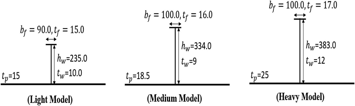
Scantlings of idealized models.
The effect of initial geometric imperfection on the ultimate strength of the stiffened panel is influenced by not only the maximum amplitude of initial imperfection but also the buckling modes of failure, including the column buckling mode, the lateral-torsional buckling mode, and the web buckling mode [21,22]. Thus, the initial geometric imperfection should be imposed concerning all possible buckling modes. Following this, the total initial geometric imperfection was defined as the sum of all the imperfections of the buckling modes, as shown in Figure 6.
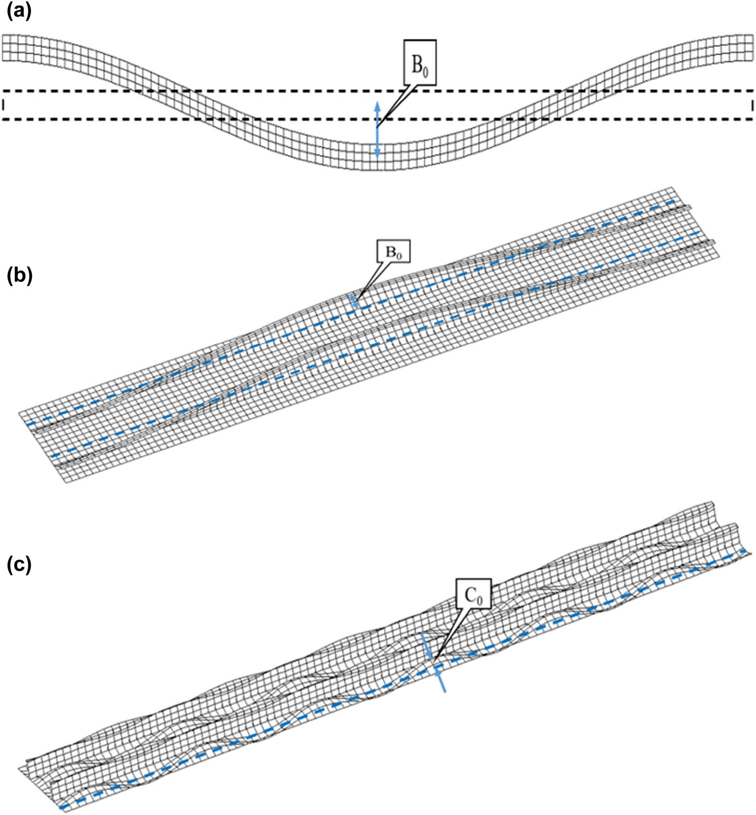
Imperfection modes: (a) column buckling mode; (b) torsional buckling mode; and (c) local buckling mode.
The formulations for generating the initial geometric imperfection are listed in Table 4.
Deformation of initial geometric imperfection
| Imperfection mode | Formulation |
|---|---|
| Column buckling |
|
| Torsional buckling |
|
| Local buckling |
|
To ensure the accuracy of the ultimate strength calculation of stiffened panels using FEM, the boundary conditions and the extent of the model must be carefully considered. The model proposed by Yao et al. [28], also used in [29], was adopted. The model is referred to as the 1/2 + 1 + 1/2 bay and 1/2 + 1 + 1/2 span model based on the covered bay and span (Figure 7).
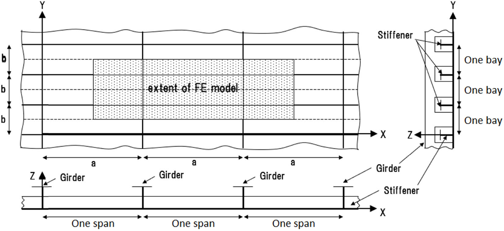
1/2 + 1 + 1/2 bay and 1/2 + 1 + 1/2 span model.
For the boundary condition, the periodic continuous condition was considered for both longitudinal and transverse edges by setting the displacements along all edges uniform, as shown in Figure 8. To simplify the calculation, the transverse frames were not modeled. Instead, their role was considered as a deflection constraint applying to the plate and the stiffener along the line of the transverse frames [29,30].
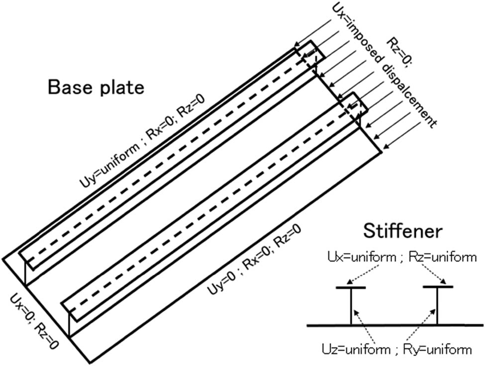
Boundary condition of FEM.
3.2.3 Corrosion
Corrosion was incorporated into the HGUS calculation as a gross thickness reduction. In reality, corrosion severity varies depending on the registered classification, country service, and cargo type. In addressing this problem, the corrosion behavior of the material was divided into two assumptions. There were a standard corrosion rate and a severe corrosion rate. The probabilistic parameters of the standard corrosion rate were calculated using all collected data from corrosion inspections up to ship ages of 25 years, while the severe corrosion rate was calculated using 95% and the above band of the total data [20]. The probabilistic parameters were described by the mean and standard deviation of corrosion rate, following a Weibull distribution for standard corrosion rate and a normal distribution for severe corrosion rate. The mean and standard deviation are listed in Table 5.
Mean value and standard distribution of corrosion rate
| No. | Member group | Standard corrosion rate (mm/year) | Severe corrosion rate (mm/year) | ||
|---|---|---|---|---|---|
| Mean | COV | Mean | COV | ||
| 1 | Bottom plate | 0.03 | 0.04 | 0.16 | 0.25 |
| 2 | Inner bottom plate | 0.13 | 0.11 | 0.33 | 0.21 |
| 3 | Lower sloping plate | 0.08 | 0.08 | 0.29 | 0.21 |
| 4 | Lower wing tank side shells | 0.04 | 0.04 | 0.15 | 0.25 |
| 5 | Side shells | 0.05 | 0.07 | 0.15 | 0.23 |
| 6 | Upper wing tank side shells | 0.04 | 0.05 | 0.17 | 0.23 |
| 7 | Upper sloping plate | 0.04 | 0.03 | 0.16 | 0.23 |
| 8 | Upper deck plates | 0.09 | 0.10 | 0.29 | 0.22 |
| 9 | Bottom girders | 0.03 | 0.05 | 0.18 | 0.23 |
| 10 | Outer bottom longitudinal – web | 0.03 | 0.02 | 0.11 | 0.22 |
| 11 | Outer bottom longitudinal – flange | 0.03 | 0.02 | 0.15 | 0.24 |
| 12 | Inner bottom longitudinal – web | 0.03 | 0.04 | 0.14 | 0.20 |
| 13 | Inner bottom longitudinal – flange | 0.03 | 0.04 | 0.17 | 0.19 |
| 14 | Upper wing tank side longitudinal – web | 0.03 | 0.06 | 0.14 | 0.21 |
| 15 | Upper wing tank side longitudinal – flange | 0.03 | 0.06 | 0.19 | 0.22 |
| 16 | Upper sloping longitudinal – web | 0.03 | 0.04 | 0.15 | 0.24 |
| 17 | Upper sloping longitudinal – flange | 0.03 | 0.04 | 0.20 | 0.23 |
| 18 | Upper deck longitudinal – web | 0.05 | 0.07 | 0.24 | 0.24 |
| 19 | Upper deck longitudinal – flange | 0.05 | 0.07 | 0.07 | 0.23 |
| 20 | Lower wing tank side longitudinal – web | 0.02 | 0.03 | 0.07 | 0.18 |
| 21 | Lower wing tank side longitudinal – flange | 0.02 | 0.03 | 0.13 | 0.18 |
| 22 | Lower sloping longitudinal – web | 0.01 | 0.02 | 0.12 | 0.18 |
| 23 | Lower sloping longitudinal – flange | 0.01 | 0.02 | 0.14 | 0.21 |
3.3 HGUS calculation results
3.3.1 Results of the initial geometric imperfection
This section aims to obtain the relationship between the inertia of the area of stiffened panel and its normalized ultimate strength for various initial imperfection conditions. The normalized ultimate strength refers to the comparison value between the ultimate strength obtained by FEA and IACS-CSR. For the first step, the load-shortening curve for all idealized models was calculated using Eqs. (1)–(4), resulting in Figures 9–11.
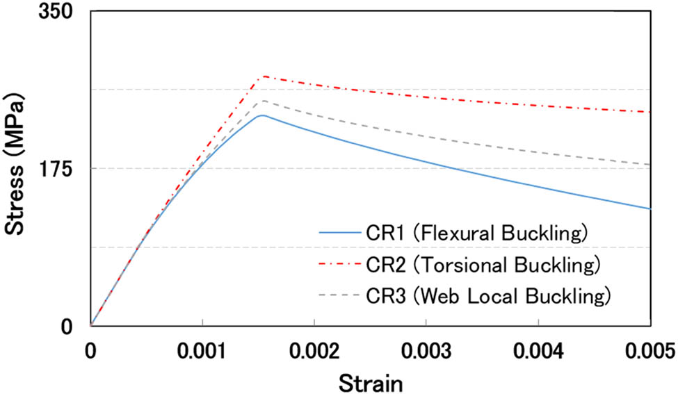
The load-shortening curve of the light model based on IACS-CSR.
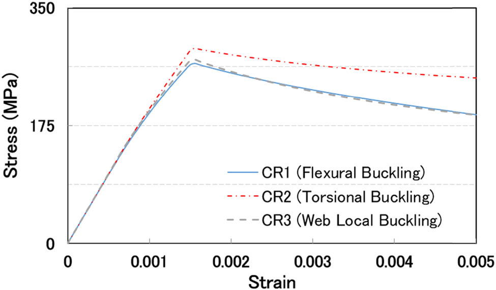
The load-shortening curve of the medium model based on IACS-CSR.
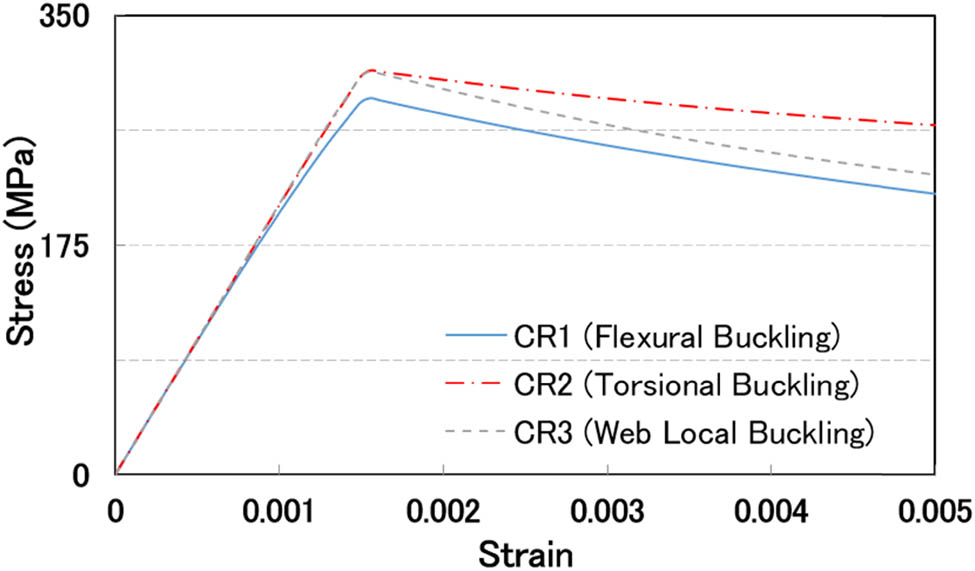
The load-shortening curve of the heavy model based on IACS-CSR.
The calculation results for all buckling modes were compared, and the ultimate strength of stiffened panels was determined as its minimum value. From Figures 9–11, it is shown that all idealized models collapsed in column buckling mode. After obtaining the ultimate strength of a stiffened panel using IACS-CSR, the ultimate strength for various initial imperfection conditions was calculated using the finite element method. The results of FEM are shown in Figure 12.
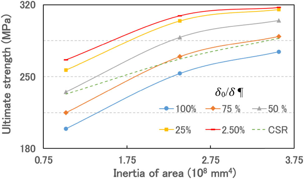
Ultimate strength for various conditions of initial imperfection by FEM.
δ is the maximum calculated initial geometric imperfection (
The next step was normalizing the FEM results in Figure 12 with the IACS-CSR results (σ/σ
CSR). The normalized value was then used as a correction factor
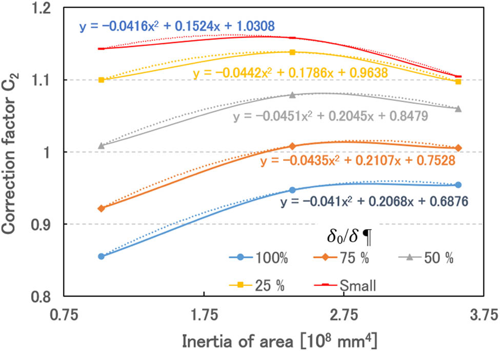
Correction factor due to initial geometric imperfection.
3.3.2 HGUS
Considering the uncertainties in material properties, geometric properties, initial geometric imperfection, and corrosion behavior and applying Monte Carlo simulation for 500 simulations per case, the distribution of HGUS versus the operation years was plotted in Figure 14 for hogging and in Figure 15 for sagging conditions, respectively. Roughly, HGUS decreases linearly in the case of a standard corrosion rate but follows a polynomial trend line in the case of a severe corrosion rate. In severe conditions, after 15 years of operation, some stiffeners had already exceeded the corrosion allowance. As stiffeners were being replaced, the decrease in HGUS for the following years slowed down.
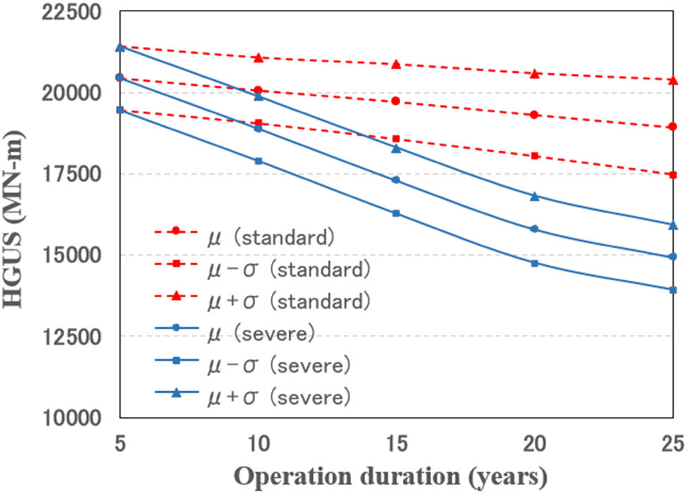
HGUS vs operation years in hogging condition.
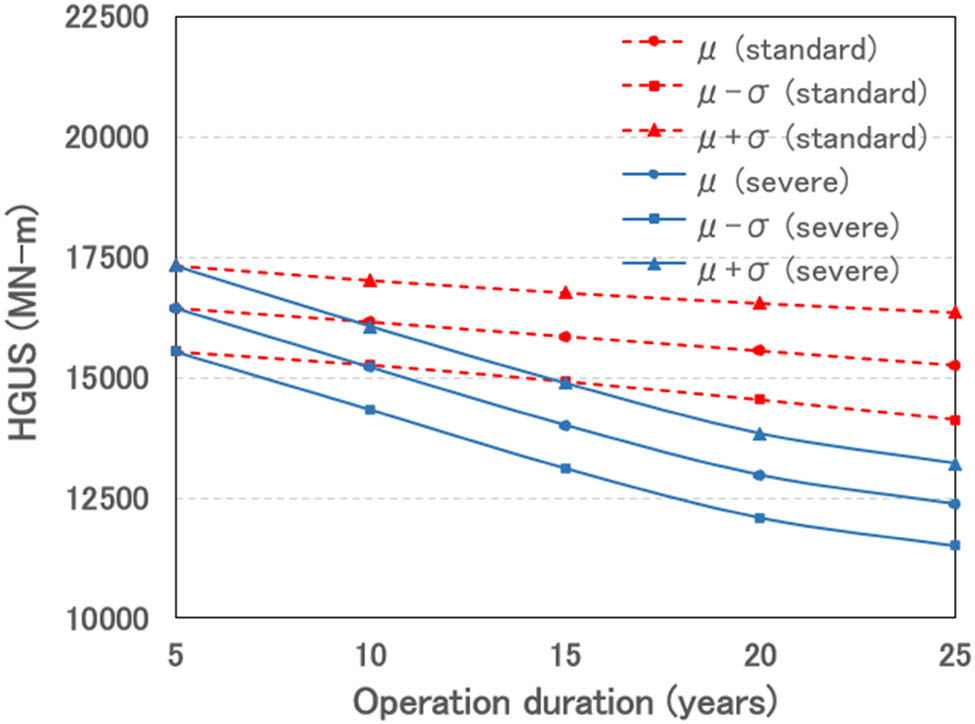
HGUS vs operation years in sagging condition.
4 Probability study on loads
4.1 Statistical description and load combination
The uncertainties associated with SWBM are caused by various factors, including loading patterns, trade routes, cargo density, and human factors. In conventional ships, SWBM generally follows a normal distribution [1]. The SWBM is defined as follows:
where
In the assessment of WIBM, the considered uncertainties are statistical uncertainties, model uncertainties, environmental uncertainties, and uncertainty due to the nonlinearity effect, which can be mathematically described as follows:
where the peaks in each wave cycle distribute according to the Weibull distribution:
where
Because SWBM and WIBM are random, their maximum values rarely coincide. As a result, the total vertical bending moment is less than the sum of SWBM and WIBM. To deal with this phenomenon, the total bending moment was calculated as Eq. (17), with the load combination factor
4.2 Uncertainties in SWBM
As Eq. (8), there are two uncertainties in SWBM calculation: model and statistical uncertainties.
where
where
4.3 Uncertainties in WIBM
The first is the statistical uncertainty
where
where
The second is the model uncertainty
Environmental uncertainty
The last is uncertainty due to the nonlinearity effect
4.4 Calculation result
In order to analyze how the total loads change over the operation period, the relationship between the increase in loads and the years of operation was plotted (see Figure 16 for the hogging condition and Figure 17 for the sagging condition).
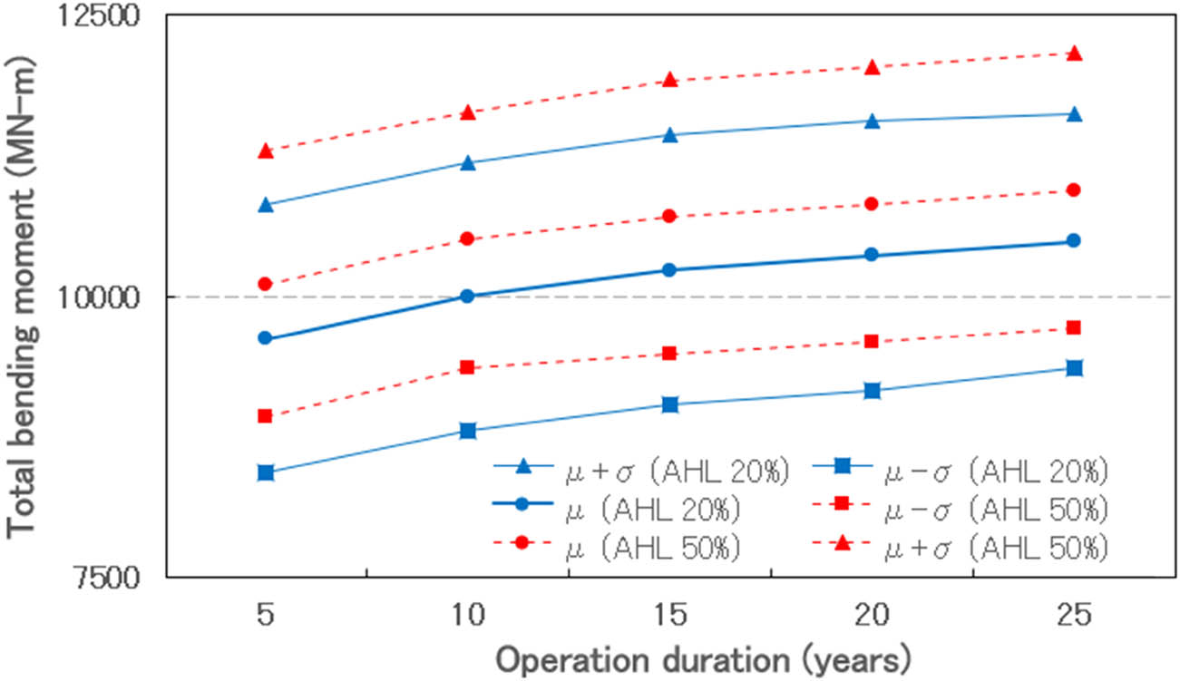
Total loads vs operation year in hogging condition.
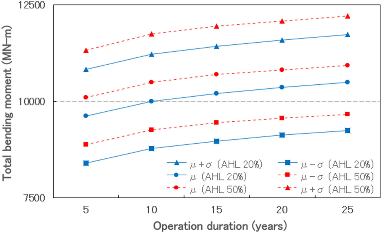
Total loads vs operation year in sagging condition.
The dashed line indicates the mean value of the total loads in the hogging and sagging conditions for an AHL duration of 50% and the straight line for an AHL duration of 20%. The lines marked with a triangle and a square show the range of majority occurrences. From Figures 16 and 17, the difference in the mean value of the total loads between the AHL duration of 20% and the AHL duration of 50% is relatively constant for all years of operation in both hogging and sagging conditions.
5 Reliability index calculation
The final step of the calculation was to determine the reliability index for each case of loading conditions. For example, Figure 18 shows the probability density function of HGUS and total loads in the hogging condition (severe corrosion rate, AHL of 50%, and 25 years of operation). The shaded area indicates the probability of failure.
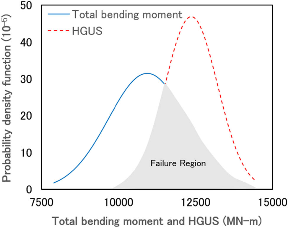
The probability density function of HGUS and total loads at severe corrosion rate, AHL 50%, and 25 years of operation.
In this regard, the reliability index is defined as follows [37,38,39]:
where
where
The reliability indexes were calculated for both hogging and sagging conditions. The results were divided into Figure 19 for the short-term duration and Figure 10 for the long-term duration, plotting the relationship between the reliability indexes vs the operation years. A short-term duration corresponds to the condition before corrosion begins (0–5 years), while a long-term duration corresponds to the condition after corrosion occurs (5 years). The blue line corresponds to the hogging condition, and the red line to the sagging condition. The straight line indicates the AHL 20%, and the dotted line indicates the AHL 50%. Figures 19 and 20 show that AHL condition and operation time reduce reliability indexes.
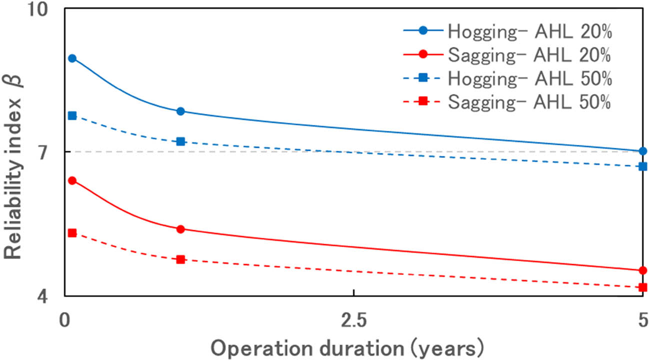
Reliability index for the short-term duration.
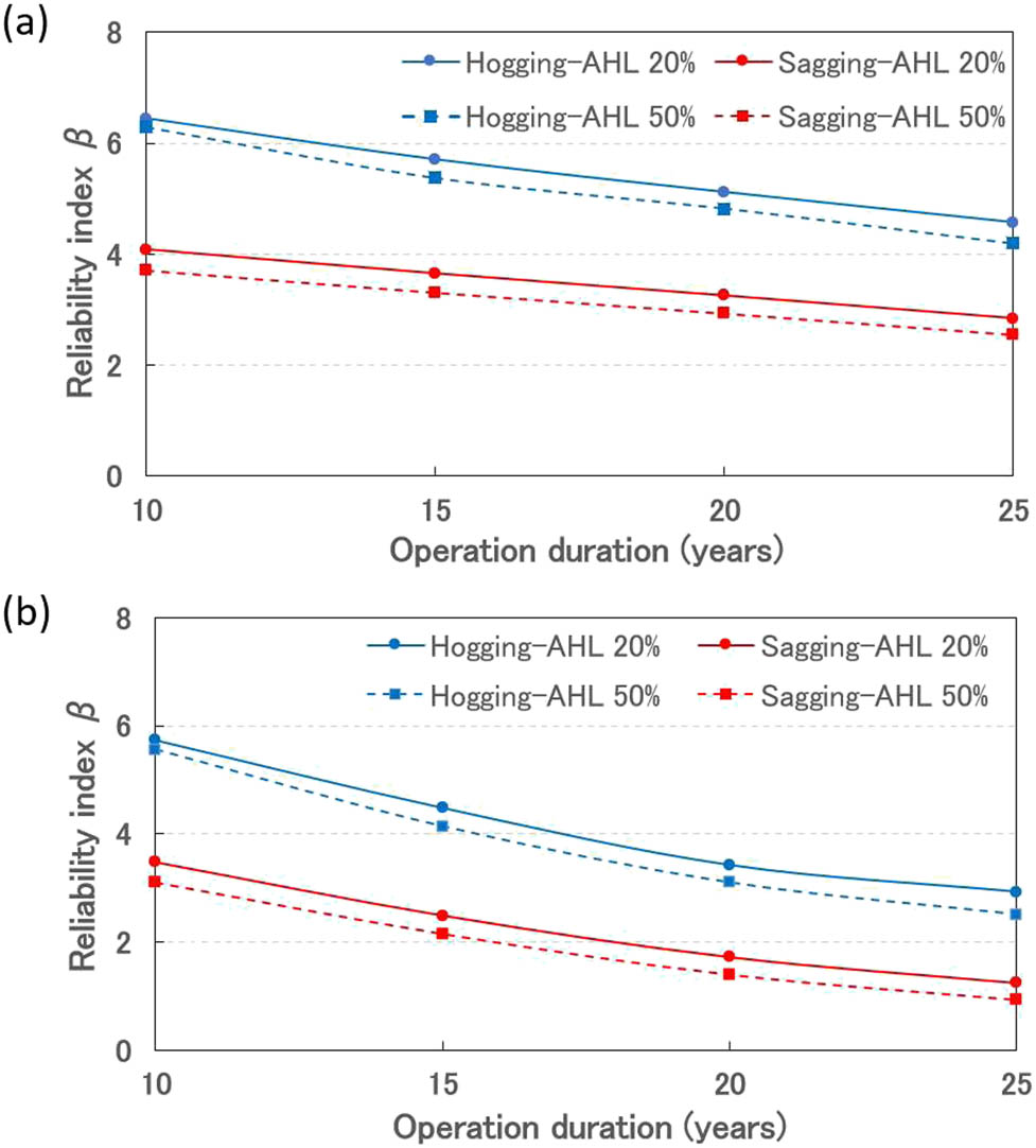
Reliability index for the long-term duration in (a) standard corrosion rate and (b) severe corrosion rate.
In Figure 19, the reliability index decreases polynomially between 1 voyage duration (23.5 days) and 1 year duration. This is because, for 1 voyage duration, the statistical uncertainty for both SWBM and WIBM was assumed to follow a normal distribution, but for operations lasting more than 1 year, they were assumed to follow the Gumbel distribution as calculated in Eqs. (19), (23), and (24) [1].
As shown in Figure 20, the reliability index for the long-term duration decreases linearly with time in the case of the standard corrosion rate, but in the case of the severe corrosion rate, the reliability index decreases along a polynomial trend line. These are the consequences of the trend of HGUS decrease, as shown in Figures 14 and 15. It can also be concluded that the effect of corrosion rate on reliability assessment is more prominent than the effect of AHL duration. Comparing the results of hogging and sagging conditions, it can be concluded that the sagging condition dominates the failure mode for bulk carriers. Thus, the hull girder’s reliability index to determine the ship’s viability is based on the reliability index in the sagging condition.
Based on ref. [40], the ideal standard reliability index for typical ship structures in the long-term duration is 2.5–3. In a condition below the target reliability index, the hull girder is in a dangerous and critical state, but if the value is much higher, the structure is overdesigned and uneconomic. According to Figure 20, after 25 years of operation, the reliability indexes of hull girders with the standard corrosion rate are 2.85 for an AHL duration of 20% and 2.55 for an AHL duration of 50%. Thus, for the standard corrosion rate, compared with a standard value of reliability index of 2.5–3, the ship could be operated for 25 years. Nevertheless, in the case of severe corrosion rate, after 15 years, the reliability index already drops below 2.5, which means that in this scenario, the ship must be maintained.
6 Conclusion
In this study, the effects of the randomness of plate thickness, stiffener size, yield strength, Young’s modulus, initial geometric imperfection, and corrosion behavior on the HGUS were analyzed for both hogging and sagging conditions. The load distribution analysis was also performed by taking into account the statistical uncertainty, model uncertainty, nonlinear uncertainty, and environmental uncertainty of the characteristic value proposed by IACS-CSR.
In the case of the HGUS calculation, the calculation was performed for the short-term duration, referring to the condition before the corrosion, and the long-term duration, corresponding to the condition after the corrosion. The corrosion behavior was also divided into two cases. The first was the standard corrosion rate and the second was the severe corrosion rate. For load analysis, there were two considerations. The first was the reference period, which was divided into short-term duration (one trip and 1 year) and long-term duration (5–25 years). The second assumption was that the duration of the ship spent in AHL condition during voyages, between 20% and 50% of voyages.
To include the effect of the initial geometric imperfection in the HGUS, equations relating the ultimate strength of a stiffened panel with the inertia of area for the various conditions of the initial geometric imperfection have been proposed. As the main results, the reliability indexes show that the sagging condition is more vulnerable than the hogging condition, and the ship could be safely operated for 25 years in the standard corrosion rate scenario but only for 15 years in the severe corrosion rate scenario.
In this analysis, the equations predicting the yield stress reduction due to initial imperfection were generated by three idealized models of stiffener elements. To increase confidence, the number of stiffener elements will be increased in future works, taking into account variations in plate slenderness, stiffener inertia, and web height. The considered type of initial imperfection will be advanced by including the initial imperfection caused by welding. Furthermore, in the reliability estimation, the higher-order reliability index will be employed to predict the structural integrity of HGUS.
Acknowledgements
This work is part of the research activity conducted by the Research Center for Hydrodynamics Technology, National Research and Innovation Agency.
-
Funding information: This research is under research grant DIPA No. 124.01.KB.6693.SDB.001.051.A. “Crashworthiness Analysis in a Fishery Patrol Vessel Collision as an Accident Mitigation During an Ambush Mission.”
-
Author contributions: Ristiyanto Adiputra (main contributor): conceptualization, methodology, calculations, formal analysis, writing – original draft, writing – review & editing, visualization.; Takao Yoshikawa (member): conceptualization, methodology, writing – review & editing; Erwandi Erwandi (member): writing – review & editing, budget acquisition.
-
Conflict of interest: The authors state that there is no conflict of interest.
-
Data availability statement: The authors declare that the data supporting the findings of this study are available within the article.
References
[1] Shu Z, Moan T. Reliability analysis of a bulk carrier in ultimate limit state under combined global and local loads in the hogging and alternate hold loading condition. Mar Struct. 2011;24(1):1–22.10.1016/j.marstruc.2010.11.002Search in Google Scholar
[2] Japan Ministry of Land, Infrastructure, Transport and Tourism. Historical data analysis in formal safety assessment of bulk carrier safety. Tokyo: MILT; 2002. Annex 3.Search in Google Scholar
[3] Roberts SE, Pettit SJ, Marlow PB. Casualties and loss of life in bulk carriers from 1980 to 2010. Mar Policy. 2013;42:223–35.10.1016/j.marpol.2013.02.011Search in Google Scholar
[4] International Association of Dry Cargo Shipowners. Bulk carrier casualty report: Years 2009 to 2018 and trends. London; 2019.Search in Google Scholar
[5] Chen N. Hull girder reliability assessment for FPSOs. Eng Struct. 2016;114:135–47.10.1201/b15120-73Search in Google Scholar
[6] Mansour A. Approximate probabilistic method of calculating ship longitudinal strength. J Ship Res. 1974;18:203–13.10.5957/jsr.1974.18.3.203Search in Google Scholar
[7] Paik JK, Kim BJ, Seo JK. Methods for ultimate limit state assessment of ships and ship-shaped offshore structures: Part I-Unstiffened plates. Ocean Eng. 2008;35(2):261–70.10.1016/j.oceaneng.2007.08.004Search in Google Scholar
[8] Gaspar B, Guedes Soares C, Teixeria AP, Wang G. Assessment of IACS-CSR implicit safety levels for buckling strength of stiffened panels for double hull tankers. Mar Struct. 2011;24:478–502.10.1016/j.marstruc.2011.06.003Search in Google Scholar
[9] Lenggana B, Prabowo A, Ubaidillah U, Imaduddin F, Surojo E, Nubli H, et al. Effects of mechanical vibration on designed steel-based plate geometries: Behavioral estimation subjected to applied material classes using finite-element method. Curved Layer Struct. 2021;8(1):225–40.10.1515/cls-2021-0021Search in Google Scholar
[10] Fajri A, Prabowo AR, Surojo E, Imaduddin F, Sohn JM, Adiputra R. Validation and verification of fatigue assessment using FE analysis: A study case on the notched cantilever beam. Procedia Struct Integr. 2021;33(C):11–8.10.1016/j.prostr.2021.10.003Search in Google Scholar
[11] Kim DK, Li S, Yoo K, Danasakaran K, Cho NK. An empirical formula to assess ultimate strength of initially deflected plate: Part 2 = combined longitudinal compression and lateral pressure. Ocean Eng. 2022;252:111112.10.1016/j.oceaneng.2022.111112Search in Google Scholar
[12] Omidali M, Khedmati MR. Reliability-based design of stiffened plates in ship structures subject to wheel patch loading. Thin-Walled Struct. 2018;127:416–24.10.1016/j.tws.2018.02.022Search in Google Scholar
[13] Seyffert HC, Kana AA, Troesch AW. Numerical investigation of response-conditioning wave techniques for short-term rare combined loading scenarios. Ocean Eng. 2020;213:107719.10.1016/j.oceaneng.2020.107719Search in Google Scholar
[14] He W, Cui X, Hu Z, Liu J, Wang C, Yao L. Probabilistic residual ultimate strength assessment of cracked unstiffened and stiffened plates under uniaxial compression. Ocean Eng. 2020;216:108197.10.1016/j.oceaneng.2020.108197Search in Google Scholar
[15] Faravelli L. Response‐surface approach for reliability analysis. J Eng Mech. 1989;115(12):2763–81.10.1061/(ASCE)0733-9399(1989)115:12(2763)Search in Google Scholar
[16] Garbatov Y, Teixeria AP. Methods of structural reliability applied to design and maintenance planning of ship hulls and floating platforms. In: Guedes Soares C, editor. Safety and reliability of industrial products, systems and structures. Milton Park, UK: Taylor & Francis; 2010. p. 191–206.10.1201/b10572-21Search in Google Scholar
[17] Guedes Soares C, Teixeria AP. Structural reliability of two bulk carrier designs. Mar Struct. 2000;13:107–28.10.1016/S0951-8339(00)00004-6Search in Google Scholar
[18] Vhanmane S, Bhattacharya B. Ultimate strength analysis of ship hull girder under random material and geometric properties. J Offshore Mech Arct Eng. 2011;133(3):031602.10.1115/OMAE2009-79887Search in Google Scholar
[19] Adiputra R, Yoshikawa T. A probability study on hull girder ultimate strength of bulk carrier considering structural uncertainties. Proceedings of the 30th Asian-Pacific Technical Exchange and Advisory Meeting on Marine Structures; 2016 Oct 10–13; Mokpo, Korea. SyDLab, 2016. p. 9–17.Search in Google Scholar
[20] Paik JK, Thayambali AK, Hwang JS. A time-dependent corrosion wastage model for bulk carrier structures. Int J Marit Eng. 2003;145:61–87.10.3940/rina.ijme.2003.a2.18031Search in Google Scholar
[21] IACS CSR. Common Structural Rules bulk carriers and oil tankers. UK: International Association of Classification Societies; 2022.Search in Google Scholar
[22] IACS CSR. Common Structural Rules, background documents. UK: International Association of Classification Societies; 2000.Search in Google Scholar
[23] Gaspar B, Teixeira AP, Guedes, Soares C. Effect of the nonlinear vertical wave-induced bending moments on the ship hull girder reliability. Ocean Eng. 2016;119:193–207.10.1016/j.oceaneng.2015.12.005Search in Google Scholar
[24] Gaspar B, Guedes Soares C. Hull girder reliability using a Monte Carlo based simulation method. Probab Eng Mech. 2013;31:65–75.10.1016/j.probengmech.2012.10.002Search in Google Scholar
[25] Gong C, Frangopol DM. Time-variant hull girder reliability considering spatial dependence of corrosion growth, geometric and material properties. Reliab Eng Syst Saf. 2020;193:106612.10.1016/j.ress.2019.106612Search in Google Scholar
[26] Piscopo V, Scamardella A. Sensitivity analysis of hull girder reliability in intact condition based on different load combination methods. Mar Struct. 2019;64:18–34.10.1016/j.marstruc.2018.10.009Search in Google Scholar
[27] Yao T, Astrup OC, Caridis P, Chen YN, Cho S-R, Dow RS, et al. Special task committee VI.2: Ultimate hull girder strength. Proceedings of the 14th International Ship and Offshore Structures Congress; 2000 Oct 2–6; Nagasaki, Japan. Elsevier, 2000. p. 321–88.Search in Google Scholar
[28] Yao T, Fujikubo M, Yanagihara D. On loading and boundary conditions for buckling/plastic collapse analysis of continuous stiffened plate by FEM. Proceedings of the 12th Asian Technical Exchange and Advisory Meeting on Marine Structures; 1998 Jul 6–9; Kanazawa, Japan. p. 305–14.Search in Google Scholar
[29] Ranji AR, Niamir N, Zarookian A. Ultimate strength of stiffened plates with pitting corrosion. Int J Nav Archit Ocean Eng. 2015;7:509–25.10.1515/ijnaoe-2015-0037Search in Google Scholar
[30] Paik JK, Kim BJ. Ultimate strength formulations for stiffened panels under combined axial load, in-plane bending and lateral pressure: a benchmark study. Thin-Walled Struct. 2002;40(1):45–83.10.1016/S0263-8231(01)00043-XSearch in Google Scholar
[31] Xu MC, Teixeira AP, Soares CG. Reliability assessment of a tanker using the model correction factor method based on the IACS-CSR requirement for hull girder ultimate strength. Probab Eng Mech. 2015;42:42–53.10.1016/j.probengmech.2015.09.003Search in Google Scholar
[32] Guedes Soares C. Stochastic models of load effects for the primary ship structure. Struct Saf. 1990;8(1–4):353–68.10.1016/0167-4730(90)90052-QSearch in Google Scholar
[33] Wirsching PH, Ferensic J, Thaymballi A. Reliability with respect to ultimate strength of a corroding ship hull. Mar Struct. 1997;10:501–18.10.1016/S0951-8339(97)00009-9Search in Google Scholar
[34] Hogben N, Dacunha NM, Olliver F. Global wave statistics. London, UK: Unwin Brothers Limited; 1986.Search in Google Scholar
[35] IACS. Standard wave data. UK: International Association of Classification Societies; 2001.Search in Google Scholar
[36] Huang W, Moan T. Analytical method of combining global longitudinal loads for ocean-going ships. Probab Eng Mech. 2008;23(1):64–75.10.1016/j.probengmech.2007.10.005Search in Google Scholar
[37] Arteaga E, Soubra A. Reliability Analysis Methods. Nantes, France: University of Nantes-GeM Laboratory; 2014.Search in Google Scholar
[38] Bai Y, Jin WL. Basics of Structural Reliability. In Marine structural design. Oxford: Elsevier Butterworth-Heinemann; 2016. p. 581–602.10.1016/B978-0-08-099997-5.00031-9Search in Google Scholar
[39] Haldar A. Fundamentals of reliability analysis. In Handbook of Probabilistic Models. Oxford: Elsevier Butterworth-Heinemann; 2019. p. 1–35.10.1016/B978-0-12-816514-0.00001-1Search in Google Scholar
[40] Mansour A. An introduction to structural reliability theory. Washington: Mansour Engineering; 1990.Search in Google Scholar
© 2023 the author(s), published by De Gruyter
This work is licensed under the Creative Commons Attribution 4.0 International License.
Articles in the same Issue
- Research Articles
- Investigation of differential shrinkage stresses in a revolution shell structure due to the evolving parameters of concrete
- Multiphysics analysis for fluid–structure interaction of blood biological flow inside three-dimensional artery
- MD-based study on the deformation process of engineered Ni–Al core–shell nanowires: Toward an understanding underlying deformation mechanisms
- Experimental measurement and numerical predictions of thickness variation and transverse stresses in a concrete ring
- Studying the effect of embedded length strength of concrete and diameter of anchor on shear performance between old and new concrete
- Evaluation of static responses for layered composite arches
- Nonlocal state-space strain gradient wave propagation of magneto thermo piezoelectric functionally graded nanobeam
- Numerical study of the FRP-concrete bond behavior under thermal variations
- Parametric study of retrofitted reinforced concrete columns with steel cages and predicting load distribution and compressive stress in columns using machine learning algorithms
- Application of soft computing in estimating primary crack spacing of reinforced concrete structures
- Identification of crack location in metallic biomaterial cantilever beam subjected to moving load base on central difference approximation
- Numerical investigations of two vibrating cylinders in uniform flow using overset mesh
- Performance analysis on the structure of the bracket mounting for hybrid converter kit: Finite-element approach
- A new finite-element procedure for vibration analysis of FGP sandwich plates resting on Kerr foundation
- Strength analysis of marine biaxial warp-knitted glass fabrics as composite laminations for ship material
- Analysis of a thick cylindrical FGM pressure vessel with variable parameters using thermoelasticity
- Structural function analysis of shear walls in sustainable assembled buildings under finite element model
- In-plane nonlinear postbuckling and buckling analysis of Lee’s frame using absolute nodal coordinate formulation
- Optimization of structural parameters and numerical simulation of stress field of composite crucible based on the indirect coupling method
- Numerical study on crushing damage and energy absorption of multi-cell glass fibre-reinforced composite panel: Application to the crash absorber design of tsunami lifeboat
- Stripped and layered fabrication of minimal surface tectonics using parametric algorithms
- A methodological approach for detecting multiple faults in wind turbine blades based on vibration signals and machine learning
- Influence of the selection of different construction materials on the stress–strain state of the track
- A coupled hygro-elastic 3D model for steady-state analysis of functionally graded plates and shells
- Comparative study of shell element formulations as NLFE parameters to forecast structural crashworthiness
- A size-dependent 3D solution of functionally graded shallow nanoshells
- Special Issue: The 2nd Thematic Symposium - Integrity of Mechanical Structure and Material - Part I
- Correlation between lamina directions and the mechanical characteristics of laminated bamboo composite for ship structure
- Reliability-based assessment of ship hull girder ultimate strength
- Finite element method on topology optimization applied to laminate composite of fuselage structure
- Dynamic response of high-speed craft bottom panels subjected to slamming loadings
- Effect of pitting corrosion position to the strength of ship bottom plate in grounding incident
- Antiballistic material, testing, and procedures of curved-layered objects: A systematic review and current milestone
- Thin-walled cylindrical shells in engineering designs and critical infrastructures: A systematic review based on the loading response
- Laminar Rayleigh–Benard convection in a closed square field with meshless radial basis function method
- Determination of cryogenic temperature loads for finite-element model of LNG bunkering ship under LNG release accident
- Roundness and slenderness effects on the dynamic characteristics of spar-type floating offshore wind turbine