A methodological approach for detecting multiple faults in wind turbine blades based on vibration signals and machine learning
-
Ahmed Ali Farhan Ogaili
 ,
Alaa Abdulhady Jaber
,
Alaa Abdulhady Jaber

Abstract
Wind turbines generate clean and renewable energy for the international market. The most important aspect of wind turbine maintenance is reducing failures, downtime, and operating and maintenance expenses. This study aims to detect multiple faults exhibited by wind turbine blades; failures such as cracks (tip crack, mid-span crack, and crack near the root) were observed in the blades at different locations. The research suggests a new approach, incorporating vibration signals and machine learning techniques to identify various failures in wind turbine blades. The technology of ranking features such as ReliefF algorithms, chi-squares, and information gains was adopted to discuss a method framework to diagnose several problems in wind turbine blades, such as cracks in different locations. The k-nearest neighbors (KNNs), support vector machines, and random forests are used to classify data based on measured vibration signals. The eight main time-domain features are calculated from the vibration signals. The proposed methodology was validated using four databases. The results showed good classification accuracy in four databases, with at least three non-conventional features in each database’s top nine features of the three classification techniques. The results also showed that when the ReliefF selection algorithm is applied with the KNN classification algorithm, it generates the highest classification accuracy under all failure conditions, and the value is 97%. Finally, the performance of the proposed classification model is compared with other machine learning classification models, and a promising result is obtained.
1 Introduction
Wind energy generated by wind turbines is becoming increasingly important as a renewable energy source worldwide. Wind turbine blades have become increasingly commonplace in recent years due to intense wind loads and material-level defects in composite systems. To produce the maximum power possible, turbine manufacturers have extended the length of turbine blades, often constructed of composite materials. Because turbine blades account for 15–20% of the total cost [1,2], it is indispensable to monitor the structural health of the blades. Repairing blade damage is one of the most expensive processes in wind turbines [3]. The failure of a blade when it occurs can cause substantial secondary damage to the wind turbine system due to rotational imbalance. Therefore, research on monitoring wind turbine blades is of utmost importance. Monitoring techniques aim to establish whether the monitored part performs the required functions, such as providing the power output as planned. It is impossible to schedule maintenance actions in advance when there is not enough information on the types of faults that occur. Specific preparations could have been made routinely or well organized before the fault if more knowledge and understanding of the flaws had been obtained.
The blades are subject to various failures caused by numerous environmental factors and massive constructions because they are exposed to air. Vibrations in the blades caused by varying wind speeds, contact with foreign objects, and various weather conditions (rain, snow, etc.) result in a delayed rotation or even failure of the turbine, which can impact total production and result in disruption. Due to the massive construction and various operating conditions, the vibration and the wind turbines’ remote location are difficult to assess [4]. The analysis of vibration signals is crucial to determine the strength and to detect and diagnose blade leaf conditions in wind turbines. Different fault diagnostic techniques using different measured variables, such as vibration [4], acoustic and noise emission [5], electrical current [6], characteristics of the generated power curve [7], etc., and signal processing, such as time domain, frequency domain, and wavelet analyses, to check the health of wind turbines (such as blades, structure, gearbox, bearings, electrical generator, etc.) and develop a maintenance plan [8]. Data-driven approaches to condition monitoring involve four fundamental steps in diagnosing wind turbine blades, gearbox, and bearing fault patterns: signal capture and conditioning, feature extraction, feature selection, and classification [9]. The signal can come from things such as vibration [10–13], thermal infrared [14], acoustic emission signals [14,15], and current [16].
Conditional monitoring includes two methods: traditional and machine learning-based methods. Traditional methods are used when there is no change in the frequency component over time. The rotating machine generates non-stationary signals since the frequency components change due to operating speed and wear and tear changes. Hence, using the traditional approach of automation systems is very difficult. Therefore, it is not desirable. In machine learning methods, algorithms can continuously learn and adapt to different situations. Consequently, researchers often resort to machine-learning approaches to diagnose mechanical system defects [17].
Various studies have been conducted on diagnosing wind turbine defects using machine learning. Abdulraheem and Al-Kindi [18] conducted a simplified investigation of cracks in wind turbine blades using experimental modal analysis. In order to simulate the blade of a wind turbine, step beams were used to study the application of experimental method analysis techniques to identify blade failures such as crack propagation. Tcherniak and Mølgaard demonstrated a structural health monitoring system based on the vibration of the blade of the Vestas V27 wind turbine [19]. They developed a plan for the structural health monitoring system to detect problems such as cracks, openings at the top and bottom edges of wind turbines, or distortions in wind turbine blades. They simulate the opening of the blade’s edge (naturally introduced) and gradually increase the size from the original 15 to 45 cm. Semi-supervised learning algorithms classify it. Sahoo et al. [20] suggested using machine learning techniques, such as K-nearest neighbor (KNN), support vector machine (SVM), and decision trees, together with captured vibration signals from turbine blades. The health conditions were healthy blades, bent blades, cracked blades, and eroded blades. According to the results, SVM had the highest identification accuracy (87%), followed by the decision tree (82%) and KNN (80.8%). Kusiak et al. [21] developed a data-driven methodology to monitor wind turbine blade pitch issues. They determined the relationships between the blade pitch flaws: blade angle asymmetry and blade angle plausibility. Bagging (72.5%), an artificial neural network (ANN) (76.2%), pruning a rule-based classification tree (75.5%), KNN (73.5%), and genetic programming (74.7%) techniques were used to conduct the study. In their analysis, only pitch faults were examined; other fault types were ignored. Joshuva et al. [22] investigated the identification and location of cracks in wind turbine blades using vibration signals. Using data from piezoelectric accelerometers, the blade reaction is calculated to construct the models when it is excited. With a multilayer perceptron classifier and a computation time of 1.51 s, the maximum number of correctly identified cases was 94.95%. Chen et al. [23] developed a model to predict wind turbine pitch failure. They acquired a classification accuracy to identify blade pitch faults. In this investigation, they also investigated pitch defects on their own. Liu et al. [24] provided a comprehensive overview of previous research on similar flaws using naive Bayes, SVMs, deep learning techniques, and the KNN. The advantages, disadvantages, and practical implications of such AII algorithms were also debated. Another review [25,26] detailed the algorithm for machine learning to detect machine problems over the years. They divide intelligent fault diagnosis algorithms into three categories: (a) traditional machine learning theories, such as probability-based graph methods, ANNs, SVMs, KNNs; (b) CNNs, raster networks, and deep learning theories, such as deep-knowledge networks; and (c) transfer learning theories, such as transfer component analysis and antagonistic genetic networks. They stated that almost all of them could be used to diagnose rotating machine problems. Both review articles focus on machine learning methods and cutting-edge techniques for diagnosing different mechanical defects rather than errors or specific mechanical defects. Sánchez et al. [27] classified gearbox and bearing problems using random forest (RF) and KNN machine learning techniques; through these, a methodical structure was discussed to detect various problems in rotating machinery. They estimated 30 time-domain features of the vibration signal using function ranking techniques such as relief, information gain (IG), and chi-square. Wang et al. [28] used multichannel convolutional neural networks (MCNN) to detect wind turbine damage using raw vibration signals automatically. This approach eliminates the need for manual inspection and analysis, thus improving efficiency and accuracy. MCNNs extract features from multiple channels of vibration data, enhancing the ability to detect and classify various types of damage. In machine learning, the information held by various features retrieved from signals is a crucial factor. Researchers employ a feature selection process in numerous applications to improve classification accuracy. The objective is to choose the most useful features based on feature ranking and eliminate irrelevant features to improve classification accuracy with the smallest possible subset of data. Wu et al. [29] used Fisher score and Mahalanobis distance techniques to select the highest-ranked feature to increase classification accuracy. Zheng et al. [30] employed another feature ranking technique, the Laplacian score, to discover informative aspects among the numerous defects. Kappaganthu and Nataraj [31] calculated statistical characteristics in the time, frequency, and time–frequency domains and used the mutual information technique to select feature sets. They discovered that classification accuracy could be significantly improved by using feature ranking techniques.
Therefore, this article compares condition monitoring indicators to find faults, such as cracks, in different locations. The experimental procedure is discussed briefly, and information about the experiment is tested under accelerated fault circumstances at various wind speeds and loads. In addition, the authors evaluated an experimental method of blade models for wind turbine blade identification based on the normal state and three common fault types: the tip of the blade crack, the blade crack in the midspan, and the blade crack at the root. An intelligent detection system is developed for wind turbines based on machine learning algorithms. The blade model for wind turbines is based on four states of fiber-reinforced polymer (FRP) blades.
The article is organized as follows: Section 2 presents common faults in wind turbine blades. Section 3 presents the methodological framework for the multi-fault diagnosis of a wind turbine blade using feature ranking methods and machine learning techniques. Experiments on wind turbine blades used to test the proposed methodological framework are described in Section 4. The findings of the diagnosis using the feature ranking in the time domain according to our framework are shown in Section 5. Section 6 indicates the outcomes for which a discussion using numbers and evidence is necessary. Section 7 provides the conclusion.
2 Common faults in the wind turbine blade
Wind turbine blades are susceptible to damage caused by both external factors and invisible defects resulting from manufacturing processes. External factors, including strong winds, rain, snow, salt fog, lightning, freezing, and storms, directly contribute to blade damage [32]. Conversely, imperceptible faults caused by manufacturing processes endure repeated high loads and severe environmental conditions during wind turbine installation and operation [33]. The gradual expansion of these invisible defects can lead to blade damage, which can be attributed to a combination of causes due to the blade’s complex materials and structure [34]. Manufacturing defects are a common cause of early blade failures, necessitating quantifying, disposing, and mitigating such defects to safeguard the current and future wind turbine fleet [33]. Defects such as dry spots, excess resin, and delamination can damage the blade [35]. Early blade failures often stem from manufacturing defects, emphasizing the importance of understanding how to measure, address, and mitigate these issues to ensure wind turbine reliability [35]. Blade damage can range from minor degradation, such as cracks and chips, to more severe problems leading to blade fracture [33]. Despite the near aerospace quality demands imposed on wind turbine blades, they are produced at considerably lower costs than comparable aerospace structures. Blade failures currently rank as the second most critical concern for wind turbine reliability [36]. Figure 1 shows some common faults in the wind turbine blades. Various techniques have been developed to detect and prevent blade damage, including computer vision-based approaches, artificial intelligence-based image analytics, and ultrasonic non-destructive testing [36]. Structural health monitoring of wind turbine blades also aids in identifying damage propagation during fatigue testing. For the wind turbine industry to create strategies that address manufacturing flaws and improve overall reliability, it is crucial to understand the factors that lead to wind turbine blade damage. Implementing strategies to mitigate blade manufacturing defects and enhance performance is paramount in ensuring wind turbine systems’ long-term operational efficiency and reliability.
![Figure 1
Common fault of the blade [32,33].](/document/doi/10.1515/cls-2022-0214/asset/graphic/j_cls-2022-0214_fig_001.jpg)
3 Methodological framework
This section presents the methodological framework utilized for analyzing the vibration signals generated by wind turbines in various operational conditions. The primary objective is to calculate a single value, known as the wind turbine blade condition index, which indicates the turbine’s overall health. This index can exhibit fluctuations, either increasing or decreasing, as the damage to the turbine worsens. It is widely recognized that faulty blades exhibit amplitude modulation at frequencies associated with specific defects. Analyzing the vibration spectrum at the characteristic frequency of a defect makes it possible to detect the presence and location of a fault. This approach forms a crucial aspect of the traditional diagnostic scheme employed, as depicted in Figure 2. To assess the effectiveness of signal characteristics in fault diagnosis, a ranking stage is employed. Three classifiers, namely RF, SVM, and KNN, are utilized to estimate the performance of the best attributes based on the accuracy achieved by each classifier. The methodological procedure, as illustrated in Figure 2, comprises the following steps:
Signal acquisition and conditioning: vibration signals from a wind turbine test rig are acquired and conditioned.
Statistical feature calculation: Eight statistical features are calculated for each signal, as outlined in Section 5.
Feature selection: The three most important features are selected from the extracted features using three different ranking techniques.
Feature ranking: The extracted features are ranked using the ReliefF algorithm, ChiSquare, and IG.
Fault classification: The RF, SVM, and KNN classifiers are utilized for fault classification.
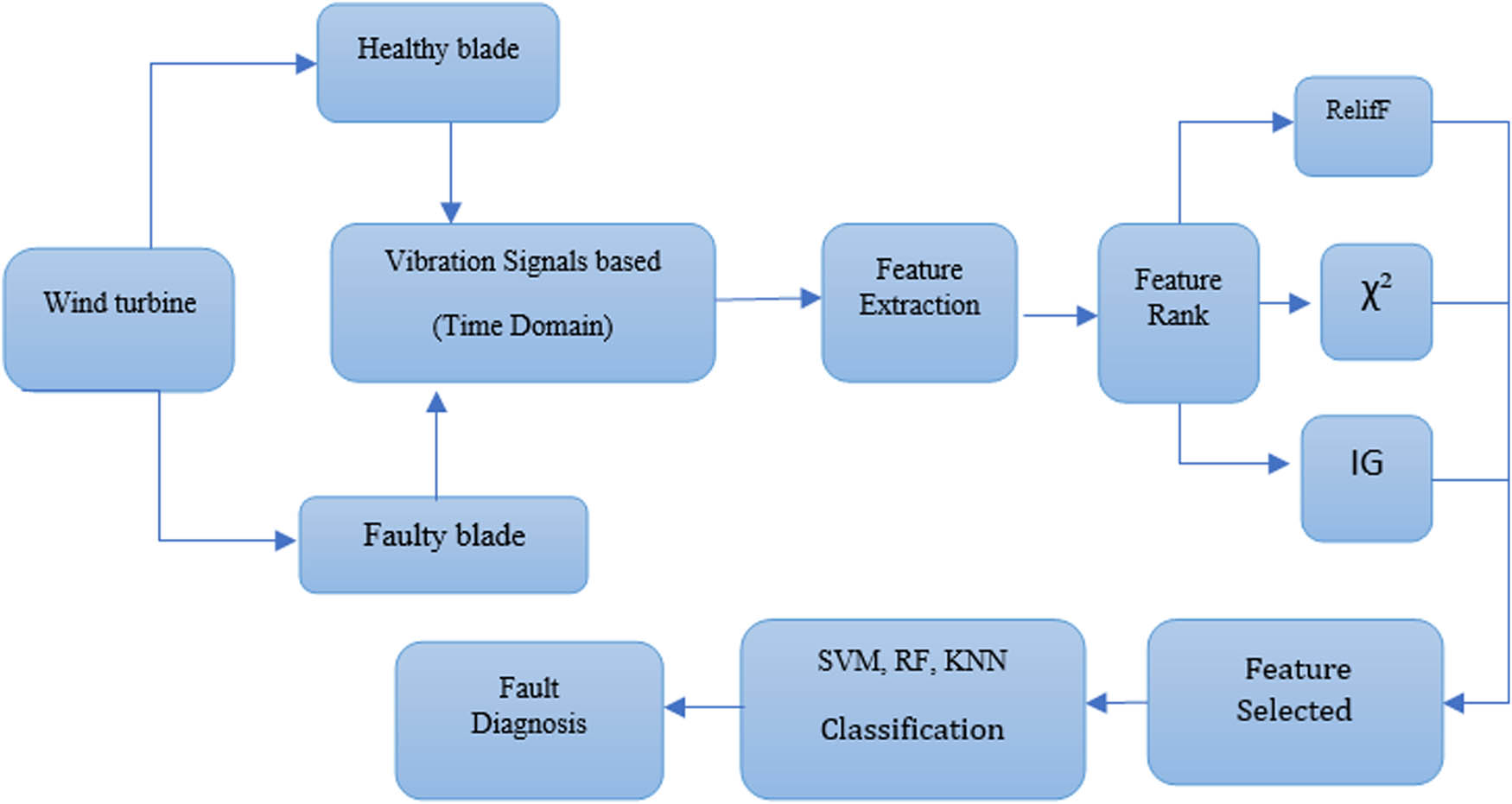
Fault detection procedure.
4 Experimental work
4.1 Experimental rig
The experimental test rig used in this study is based on a wind turbine blade and utilizes the Computer-Controlled Wind Energy Unit (EEEC) provided by Edibon Equipment, as shown in Figure 3(a). It comprises a laboratory-scaled aerogenerator with a rotor, generator, and computer-controlled axial fan. The rig allows air velocity control by adjusting the rotational speed and offers flexibility in blade configuration. The set-up includes a stainless steel tunnel with transparent windows to simulate natural wind conditions, with wind tunnel velocities ranging from 1.3 to 5.3 m/s. The aerogenerator has a diameter of 510 mm and generates 60 W of power with a maximum voltage of approximately 12 V and an operational charging current of 5 A.

Installation of the wind turbine system (a) EEEC wind turbine, (b) accelerometer attached to the turbine hub, and (c) DAQ of the DAQ model NI-USB-4431.
In the experimental design, as depicted in Figure 4(b) and (c), a piezoelectric accelerometer was employed as a transducer to capture vibration signals. This sensor is well-suited for detecting faults at high frequencies and is commonly used in condition monitoring. The specific accelerometer model utilized in the study is the PCB Piezotronics 352C65 uniaxial accelerometer; its specification is shown in Table 1. An adhesive mounting technique was employed to securely install the accelerometer on the nacelle near the wind turbine hub, enabling vibration data collection.
The simulated faults in the blades.
Specification of the uniaxial PCB Piezotronics 352C65 accelerometer
| Property | Value |
|---|---|
| Sensitivity | (±10%) 100 mV/g (10.2 mV/(m/s²)) |
| Measurement range | ±50 g pk (±491 m/s² pk) |
| Broadband resolution | 0.00016 g rms (0.0015 m/s² rms) |
| Frequency range | (±5%) 0.5 to 10,000 Hz |
| Weight | 0.070 oz (2.0 g) |
A cable connected the accelerometer to the data acquisition (DAQ) card. The NI USB 4431 DAQ card was utilized in the study, featuring five analog input channels, a sampling rate of 102.4 kS/s, and a resolution of 24 bits. The accelerometers and the DAQ devices interfaced to a Lenovo laptop equipped with Core i7 CPUs. The DAQ process was facilitated using LabVIEW software.
4.2 Experimental procedure
Initially, the wind turbine was healthy (without defects); the accelerometer was used to record the signals. These signals were captured using the listed requirements:
1. The sample length was established to maintain consistency, and the following factors were also considered. Statistical measures are more relevant when the number of samples is large enough. On the contrary, as the number of samples increases, so does the computation time. According to the Nyquist sampling theorem, the sampling frequency must be at least twice the maximum frequency to achieve balance [37]. Hence, the sampling rate was set at 1,000 Hz.
2. A minimum of 500 samples were collected for each state of the wind turbine blade, and vibration signals were recorded using LabVIEW 2020.
The turbine was operated at 240 rpm. The accelerometer is positioned vertically on top of the hub to monitor vibrations (y-axis), as illustrated in Figure 3(b). DAQ is used to gather vibration signals at a sampling rate of 1,000 Hz and a sample size of 500. This results in four rotations (240/60 ≈
4.3 Intentionally adopted faults
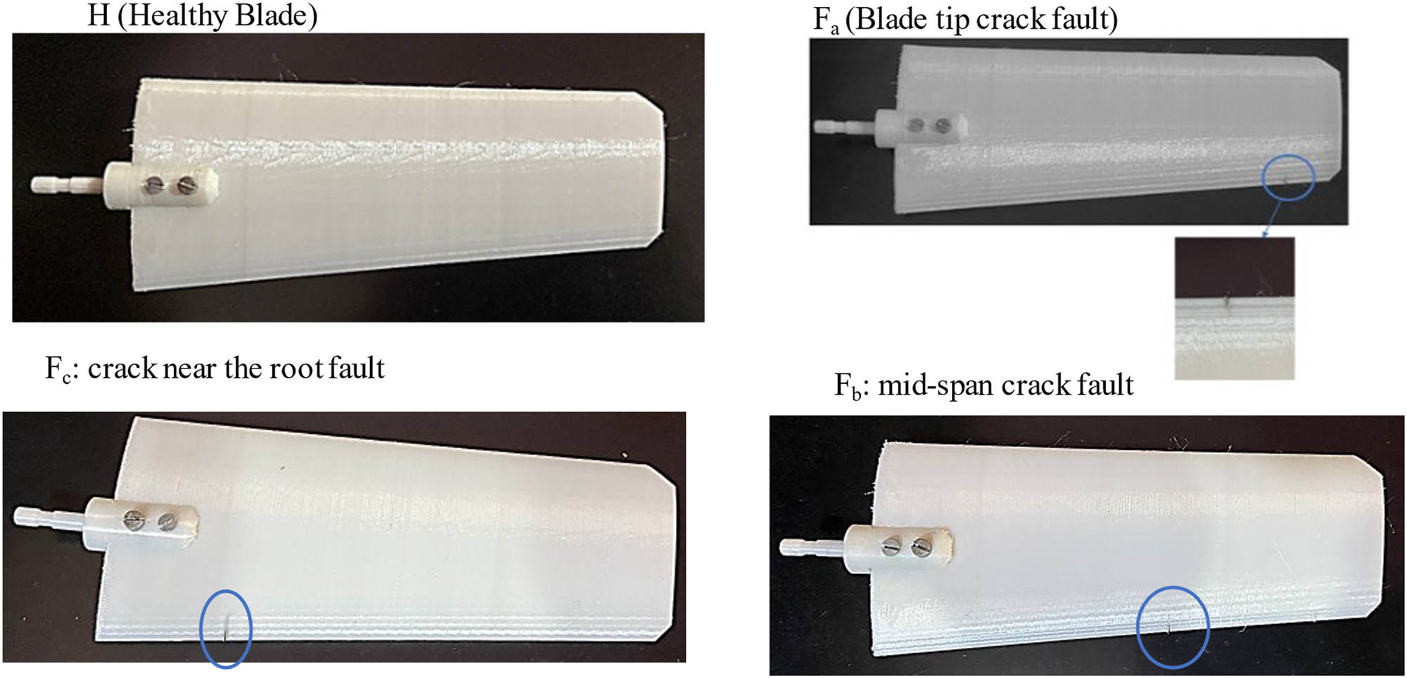
In this research, we created models of wind turbine blades based on normal conditions and common blade fault states (cracks with different locations) to discuss the vibration signals generated by wind turbine blades in various states. The blades in this study were custom-designed by the manufacturer of genuine commercial wind turbines. The blades were made of FRP, measured 300 mm long, and were solid from the inside. Figure 4 shows the three simulated fault types in addition to the healthy case of the blades used in this investigation. This study defines three fault types such as Fa: Blade tip crack fault, Fb: mid-span crack fault, and Fc: crack near the root fault.
5 Feature extraction and selection
Wind turbine vibration signals are nonlinear, necessitating appropriate signal processing techniques for accurate analysis of component health. This study extracts the vibration signal’s features using time-domain signal analysis [38]. Signals in the time domain can be analyzed directly by observing their patterns, simplifying calculations. The time-domain characteristics are computed directly from the time waveform of the signal. Typically, time-domain signals contain valuable information regarding temporal amplitude changes. Analyzing these signals is economical, requiring only fundamental signal conditioning as preprocessing. The analysis entails visually examining sections of the time waveform and identifying any anomalous behavior. However, visual inspection alone is unlikely to detect defects due to multiple components in machine-generated vibration signals that are difficult to distinguish in the time domain.
Consequently, statistical data, known as condition indicators, are gathered and compared to predetermined criteria to determine whether the machine is operating normally or exhibiting abnormalities. These statistical features are utilized for the fault diagnosis of wind turbine blades. Below is a brief explanation of these statistical features [17–20,22–39]:
Kurtosis: It measures the degree of peakedness or flatness of a distribution. It is calculated by taking the sum of the fourth power of the deviations from the mean and dividing it by the square of the standard deviation.
(1)Root mean square (RMS): A mathematical metric that calculates the square root of the average of the squared values within a dataset. It is a reliable measure to assess a signal’s overall magnitude or amplitude. This widely employed technique allows for quantitative analysis of signal strength and intensity.
(2)Variance: It measures the average squared deviation from the mean in a dataset. It provides a measure of the spread or dispersion of the data points.
(3)Standard deviation (σ): It is the square root of the variance and provides a measure of the dispersion of data around the mean. It quantifies the average amount of deviation or variability in a dataset.
(4)V max: It represents the maximum value observed in a given signal.
(5)Skewness: It measures the asymmetry of a distribution. It is calculated by taking the sum of the cubed deviations from the mean and dividing it by the cubed standard deviation.
Crest factor: It is the ratio of the maximum value (V max) to the RMS value of a dataset. It is commonly used to assess the peak-to-average ratio of a signal.
Mean (µ): It represents the average value of a dataset. It is calculated by summing all the values and dividing by the total number of data points (N).
where x i is a signal for i = 1, 2, N, N is the number of data points.
5.1 Feature selection
Before pattern recognition, selecting features is crucial because it eliminates loud, redundant, or unnecessary features, significantly reducing the number of features. In most cases, it optimizes classification tasks and improves the performance of learning algorithms. In the diagnosis procedure, selecting the appropriate features or collecting features that reflect the device’s condition is important. It is believed that a good feature or set of features allows one to distinguish between normal and abnormal circumstances, enabling trend analysis while avoiding the impact of other device operating parameters [36]. In most cases, selecting features is considered a dimension-reduction problem. Techniques such as principal component analysis, multidimensional scale, factor analysis, projection search, and kernel Fisher discrimination analysis are used. However, these methods usually produce synthetic properties greater than the original set, so the reduced set properties are not of physical importance [37,40]. Fisher’s scores, ReliefF algorithms, Wilcoxon ranks, gains ratios, memetic characteristics selection, chi-squares, and IGs are used to select relevant characteristics and improve precision in the diagnosis of mechanical failures [41–43].
5.2 ReliefF algorithm
ReliefF is a supervised feature classification algorithm [44]. It is typically used in data preprocessing to select feature subsets. ReliefF is based on randomly generating instances, computing their nearest neighbors, and adjusting a feature weighting vector to provide greater weight to attributes that distinguish the instance from neighbors of other classes. It is an extension of the Relief approach (used for binary classification) that aims to evaluate the quality of the distinguishing factors of neighboring samples [45]. The ReliefF algorithm begins by selecting a random instance, followed by a search for the k nearest instances of the same class. This operation alters a weighting vector (W) that gives greater weight to traits that better differentiate between surrounding groups and is defined by [46]:
where W f represents the weight of the feature f.
5.3 Chi-square (χ²)
The chi-square statistical optimal feature selection approach was used to improve prediction accuracy [47]. Feature ranking allows testing to determine whether a specific feature’s occurrence and a specific class’s occurrence are independent. Thus, when a feature is independent of the class, this is discarded [48]. It can be computed as follows:
In this equation, χ² represents the chi-square statistic, and the summation symbol (∑) signifies that the equation is computed for each category or cell in the dataset. u j denotes the observed frequency in each category or cell, while u j represents the expected frequency in each category or cell, assuming no association exists between the variables.
5.4 IG
IG is a crucial metric in machine learning for evaluating feature relevance in classification tasks [43–49]. It measures the reduction in entropy when a feature is known. The IG for a feature is calculated as the difference between the entropy of the original dataset and the weighted average of the entropies of the subsets created by splitting the dataset based on that feature. The equation for IG is
where IG(F) is the IG for feature F, H(D) is the entropy of the original dataset, |Dv| represents the number of instances in each subset, and H(Dv) is the entropy of each subset. Decision trees use IG to determine feature selection order, selecting features with higher IG as more relevant for accurate classification. Alternative metrics like gain ratio and Gini index address limitations of IG. Overall, IG quantifies the reduction in entropy and aids in identifying informative features for classification.
6 Machine learning
This section presents an overview of three prominent machine learning algorithms commonly employed for fault classification. SVM, KNN, and RF. These algorithms have demonstrated effectiveness in various domains, including fault diagnosis and detection in rotating machinery.
6.1 SVM
SVM is a supervised learning algorithm mainly used for classification and regression. Vapnik described the theoretical concepts of SVMs [50]. Due to its high precision and good generalizability, some researchers [51,52] have used SVM to classify mechanical failures in rotating machines, even if the sample is small. The formulation of the SVM is based on the principle of minimization of structural risk. For binary classification problems, the aim is to maximize the margin between the different planes. The maximum margin to separate hyperplanes (H 1) can be used to classify the data sets into the classes to be considered. The equation of H 1 can be written as follows.
where x is the point on the separator plane (H1), and w is the vector on the plane. Normalization of the two-class w parameters can be represented as
and
By combining Eqs. (13) and (14), we obtain the following:
where ξ i represents the slack parameter.
Due to better generalization capabilities, SVM is of great interest to academic and industrial societies as an algorithm for fault detection systems.
6.2 KNN
The KNN algorithm is a supervised learning approach used for classification and regression tasks. It is a nonparametric model that utilizes training datasets to classify new samples from test datasets based on nearest-neighbor criteria [53]. The algorithm searches for k samples in the training set that is closest to the new test sample. Classification is then based on the most prevalent classes among the nearest neighbors. Given a training set D(x, y) where x represents a sample and y its corresponding class, and a test sample z = (x′, y′), the algorithm calculates the distance between z and all training samples (x, y) in D to obtain a list of nearest neighbors [54]. The class assignment for y corresponding to the test sample x is determined by a majority vote of the neighboring classes.
The class assignment equation can be expressed as follows:
where v represents a class label, yᵢ denotes the neighboring class label, and I is an indicator function that returns 1 if the condition in parentheses is true. This equation allows for the determination of the class with the highest frequency among the neighboring samples.
In some cases, a weighted approach is used to account for the contribution of each neighboring sample based on its distance from the sample to be classified. The weight factor can be defined as the inverse square of the distance:
In this manner, the kNN algorithm can be defined as follows:
Another important consideration in the kNN algorithm is the choice of distance metric. The most common distance metric used is the Euclidean distance, but alternative metrics such as cosine similarity, Minkowski distance, correlation, and chi-square distance can also be employed [55].
In summary, the kNN algorithm utilizes nearest-neighbor principles to classify new samples based on their proximity to training samples. The class assignment is determined through majority voting, and a distance metric is used to measure the similarity between samples [56].
6.3 RF
RF is a machine-learning technique introduced by Breiman [57] that leverages an ensemble of decision trees. By combining the concepts of bagging and random feature selection, RF aims to address issues related to variance and overfitting. In this approach, each tree in the forest independently determines the class for a given sample, and the final class prediction is made through majority voting. The training data used to construct each tree are referred to as the “in-bag” data, while the remaining data constitute the “out-of-bag” observations (OOB) [58]. OOBt represents the OOB sample associated with tree t. The classification error of the forest, errForest, can be defined as follows:
where
6.4 Evaluating the machine learning model
Developing a machine learning model is a crucial skill for aspiring data scientists. However, the initial model is rarely the “best” model. Evaluating the quality of our machine learning model is crucial for improving its performance until it reaches its maximum potential. Evaluation metrics for classification problems compare the expected class label to the predicted class label or interpret the predicted probabilities for class labels. Classification problems are widespread and have numerous applications in the real world, such as identifying spam emails, targeting marketing, fraud detection, and determining whether a patient is at high risk of having a particular disease diagnosis. In this blog article, we examine various categorization evaluation metrics that can be applied to issues of this nature.
Confusion matrix (CM)
The CM is crucial in classification tasks, summarizing the predicted and observed values. It represents four outcome combinations and enables evaluation using precision, recall, accuracy, F1 score, and area under the curve (AUC)-receiver operating characteristics (ROC) metrics. Engineers and professionals in the wind industry rely on the accuracy and interpretability of the proposed model, which is visualized in a table-like format. The CM provides count values for accurate and inaccurate predictions, allowing for analysis and decision-making. Overall, the CM is a valuable asset for evaluating classification models in various fields, including the wind industry.
Precision is the number of classified correct outputs or the exactness of the model. It is calculated using the following equation:
(20)Recall: Recall is our model’s measurement to identify the real positive. The calculation is done using the following equation:
(21)Accuracy: Accuracy is the percentage of production that is correctly predicted. Measure how many positive and negative observations were correctly classified. Calculations are made using the following equation:
(22)F 1 score: The F1 score is an average of accuracy and recall. They combine accuracy and memory into a single metric by calculating their harmony average. The formula is calculated using the following equation:
(23)Specificity, S , also called the true negative rate, measures the proportion of negatives that are correctly identified, given by the following equation:
(24)where T p represents actual positive values, T n represents valid negative values, F p represents false positive values, and F n represents false negative values.
ROC
The ROC based on the CM is used to evaluate the classification. The ROC curve extracts many indices to assess a classifier’s effectiveness. The region between the ROC curve and the negative diagonal is the AUC, with a value between 0.5 and 1 [59,60]. Because there is an area where the value of R and P is 1 for each cutoff point, AUC = 1 implies a perfect rating, while AUC = 0.5 shows that the classifier is faulty. The Wilcoxon rank test and AUC’s statistical characteristics are equal [61]. The Gini coefficient [62] is twice the area between the diagonal and the ROC curve, and the AUC is also closely connected.
7 Results and discussion
This study aimed to evaluate a methodological framework to classify features in the multi-fault diagnosis of rotating equipment using RF, KNN, and SVM classifiers and determine the importance of non-conventional features in wind turbine fault diagnosis processes. The datasets were utilized to test the technique and significance of the four non-standard characteristics.
7.1 Time domain vibration signals analysis
In the present study, the state of the wind turbine blades included standard blades and blades with various faults. The wind turbine blades rotated at various wind speeds during health state detection. The blades rotated at a wind speed of (1.3–5.3) m/s, which is compatible with the Iraqi climb [2]. Recent research [16–25] has used vibration signals extensively due to their efficiency in forecasting difficulties. Using NI LabView signal processing software, accelerometer voltage values were collected and converted to time-domain acceleration signals. Figure 5 shows the reference vibration signals of the healthy blade and another blade with fault condition signals taken when different cracks in the wind turbine blade at different wind speeds. They show the vibration signal plot (time vs amplitude) for a healthy condition blade, Fa (blade tip crack fault), Fb (blade mid-span crack fault), and Fc (blade root crack fault), respectively. This gives a basic idea about how the magnitude of the acquired vibration signal varies over time concerning simulated faults. It was observed that the vibration signals changed depending on wind speed, from Figure 5, V wind = 1.3 m/s observed the vibration signals in the healthy case. Normally, a slight vibration would occur during the operation; therefore, the vibration measure. Therefore, the observed signals suggested that the wind turbine was operating normally. While observed, the signals changed and were affected by the type of faults. It can be seen that the signs change significantly compared to the rest of the cases. The increase in wind speed to reach 3.3 m/s observed the vibration signals for the blade with a crack near the tip more affected by another. It was repeated when the wind speed increased to reach 5.3 m/s. Time-dominant vibration signals provide the key indication of wind turbine faults.

Blade vibration signatures.
7.2 Result of the feature ranking
Eight-time domains are measured from the vibration signals of the wind turbine. They are input to machine learning algorithms for fault classification [34]. Three feature ranking algorithms were used to optimize the feature set, viz. the IG Chi-square (χ²) and ReliefF reduce the order of the set of features. Table 2 compares the results of the feature ranking algorithms and shows how the calculated features are ranked. Variance, standard deviation, and RMS are the best-ranked features based on IG, and variation is the most helpful feature. Although using Chi-square (χ²) to rank the characteristics, kurtosis, skewness, and RM were the most important. The kurtosis value in the time domain was the most important feature since it shows the average power of the measured signal and is given more weight than the other features.
Ranking results for each data set
| Rank algorithms | Info. gain (IG) | Chi χ² | ReliefF |
|---|---|---|---|
| Features | Variance | Kurtosis | Standard deviation |
| Standard deviation | Skewness | Variance | |
| RMS | RMS | Skewness |
Furthermore, Table 2 displays the ranked feature list generated by the ReliefF algorithm, which is utilized to demonstrate further the utility of the feature ranking method for fault classification and observed that the standard deviation and the variance and value become the most significant of the ten measured features. It is observed from Table 2 that the standard deviation features are more significant compared to other time domain features. Where it appears in each algorithm, the measure of the vibration signal’s actual energy or power content is weighted high compared to the other feature. The same observation is also found in Table 2. Using the RF-ranked feature set, two classifiers compare the classification accuracy with selected features. In the current study, the classification of features depends on the time domain from which the characteristics are calculated and the weight assigned by the ranking method.
7.3 Result of machine learning
This study focuses on the application of three widely used machine learning algorithms, namely SVM, KNN, and RF, to detect faults in wind turbine blades. Additionally, the integration of feature ranking techniques, specifically IG (IG), Chi-square (χ²), and ReliefF, is employed to identify the most effective methodology for integrating machine learning models. The objective is to identify the optimal combination of algorithms and feature ranking methods to enhance the accuracy and efficiency of fault detection in wind turbine blades.
The confusion matrices presented in this study illustrate the performance of three different types of machine learning algorithms, namely KNN, SVM, and RF, in classifying instances into four categories: Fa (crack at tip blade), Fb (crack at mid-span blade), Fc (crack near the blade root), and H (healthy state). The confusion matrices display the number of instances predicted for each category and compare them to the actual distribution of instances.
Table 3 presents the confusion matrices for the three machine learning algorithms (kNN, RF, SVM) when applying the IG feature ranking method. Each matrix shows the number of instances classified into different categories: Fa (crack at tip blade), Fb (crack at mid-span blade), Fc (crack near the blade root), and H (healthy state). The numbers in the matrix represent the count of instances correctly classified and misclassified for each category. For example, in the kNN CM, there are 963 instances of Fa correctly classified, 482 instances misclassified as Fb, 202 instances misclassified as Fc, and 453 instances misclassified as Healthy.
Comparison of the evaluation matrices with other models for Info. gain
 |
The Chi-square feature ranking method was employed as the second approach for fault selection in wind turbine blades. Table 4 presents the confusion matrices for each model utilizing the chi-square feature ranking. Within the confusion matrices, the diagonal elements represent correctly identified instances, while the off-diagonal elements indicate misclassifications. In this context, Fa corresponds to the root crack, Fb denotes the mid-span crack, and Fc represents the crack at the blade’s tip. The classification accuracy for the KNN model is 58.4097%, with 583.785 instances misclassified as Fb and 584.505 instances misclassified as Fc. Outperforming the kNN model, the SVM model achieves an accuracy of 79.8953% and correctly classifies 789.53 instances as Fb, yielding an F1 score of 0.798075. Similarly, the RF model demonstrates strong performance with an accuracy of 79.8456% and an F1 score of 0.798456.
Comparison of the evaluation matrices with other models for the Chi-square
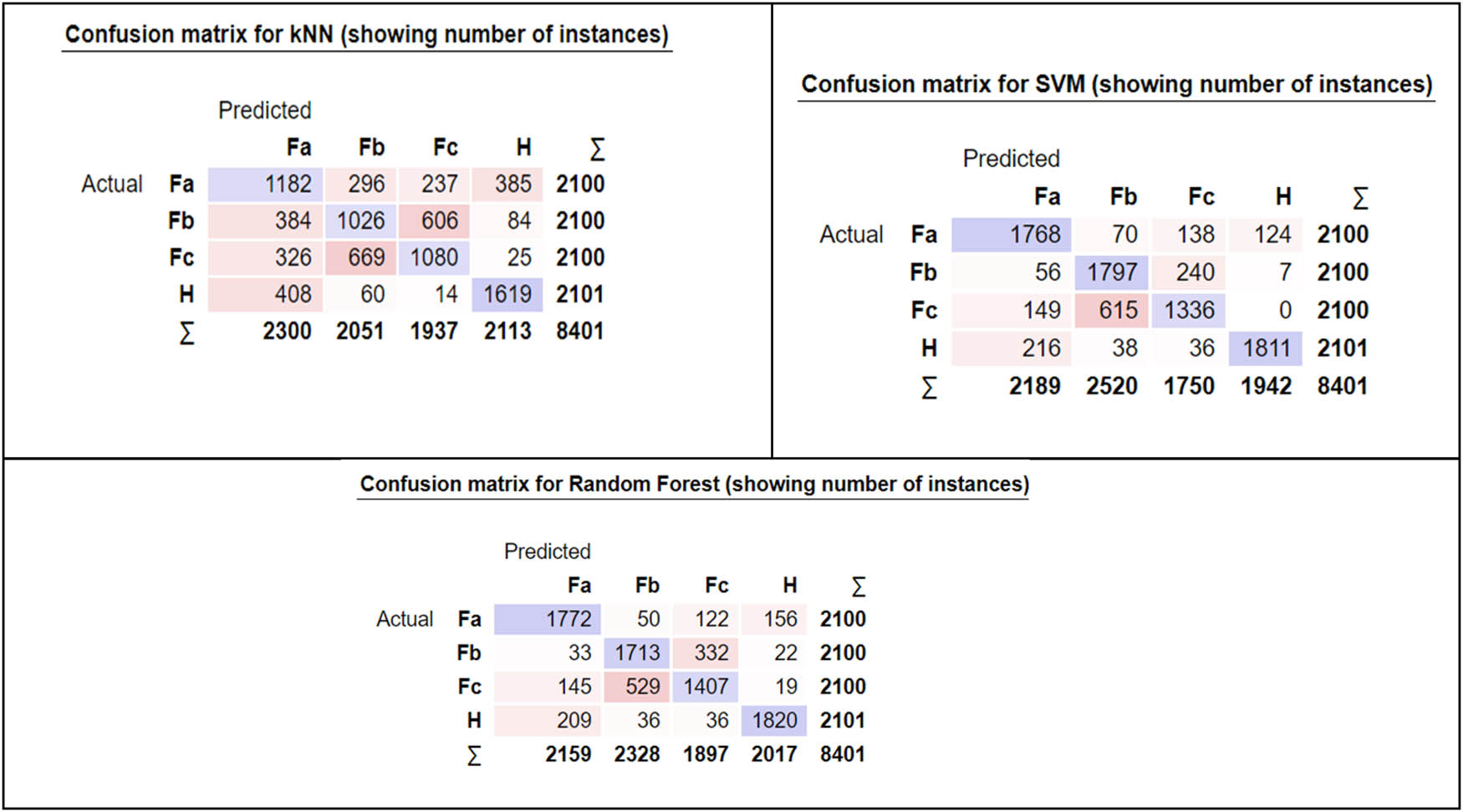 |
These findings emphasize the efficacy of the chi-square feature ranking method in accurately identifying faults in wind turbine blades. The kNN model exhibits moderate accuracy but encounters challenges in distinguishing between Fb and Fc instances, resulting in a significant number of misclassifications. On the other hand, the SVM and RF models showcase superior performance in correctly classifying Fb instances. Further investigations can delve into optimizing these models, refining feature selection techniques, and exploring ensemble methods to enhance the overall accuracy and robustness of the fault classification systems.
Table 5 displays the results of applying the ReliefF algorithm to three machine learning models: SVM, KNN, and RF. Table 5 presents confusion matrices, indicating the number of instances classified into categories representing blade conditions (H: healthy, Fa: crack at tip blade, Fb: crack at mid-span blade, and Fc: crack near blade root). SVM achieved accurate classification for Fa in 1,344 instances but misclassified 127 Fa instances as Fb, 108 as Fc, and 521 as H. kNN achieved perfect classification for the Healthy state (H) and accurate Fa classification for 2,083 instances. RF accurately identified Fa (1,997 instances) but misclassified some instances across other states. These matrices provide valuable insights into the performance of each algorithm, facilitating analysis of accuracy and misclassification patterns.
Fault CM for ReliefF
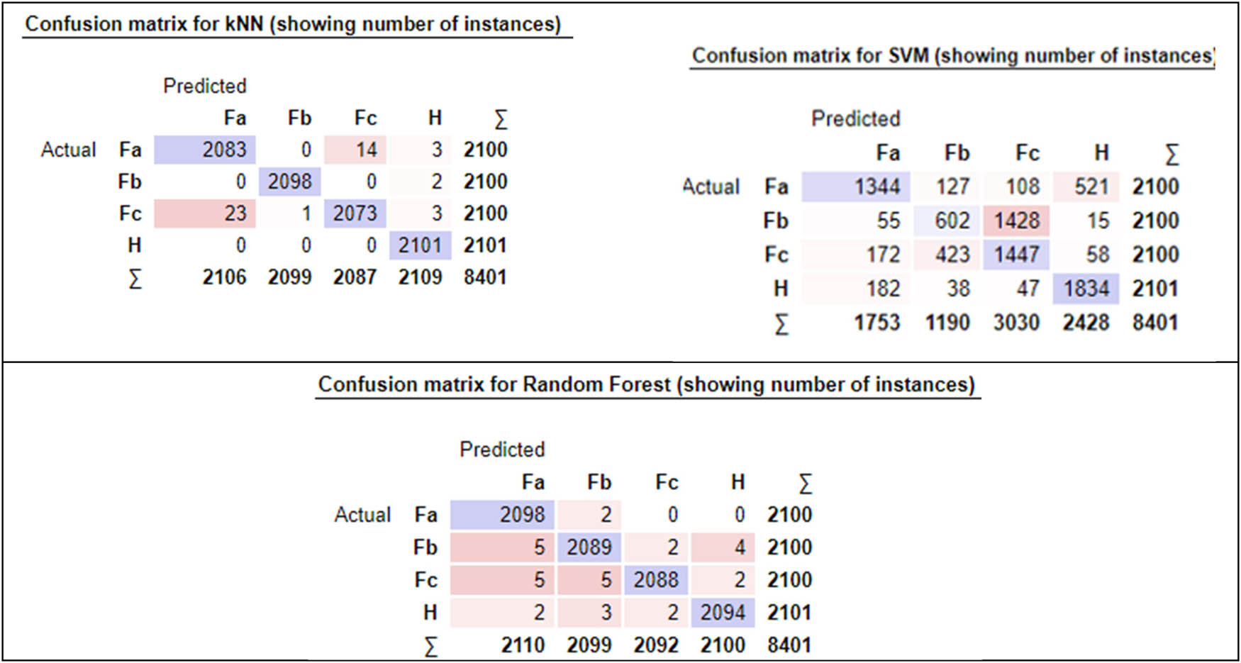 |
The results obtained from the machine learning models for wind turbine blade fault detection demonstrate remarkable advancements in accuracy and precision. The application of the ReliefF feature ranking method yielded an impressive classification accuracy of 97%, surpassing the accuracy reported in the reference [61], which achieved a maximum of 94.94% accuracy [22]. Furthermore, the proposed hierarchical feature selection approach based on relative dependency exhibited a remarkable classification accuracy of 97.08% for gear fault diagnosis, as documented in the study of Manju et al. [63]. The utilization of multimodal deep support vectors with homologous features for gearbox malfunction diagnosis also showcased exceptional performance, with accuracy exceeding 97% using any of the four ranking features for the RF and kNN classifiers [63,64]. Comparatively, the precision achieved by these models ranged from 96.7 to 97%, outperforming the precision values reported in previous studies [63,64].
Table 6 provides a comprehensive overview of the precision values obtained by the kNN classifiers, revealing that the IG feature selection method resulted in the lowest precision, plunging as low as 54.0649%. Conversely, the ReliefF feature ranking method consistently yielded the highest precision and delivered superior results across all fault classifications. Table 6 further supports these findings, demonstrating that the IG algorithm yielded the lowest precision value, while the employment of ReliefF resulted in the highest precision and recall values. These results are congruent with the F score and AUC metrics, affirming the efficacy of the ReliefF algorithm for feature selection in identifying the most critical features and achieving exceptional precision in fault classification, as corroborated by prior research [65].
Comparison of the evaluation matrices with other models
| Model | AUC | CA | F1 | Precision | Recall | LogLoss | Specificity |
|---|---|---|---|---|---|---|---|
| Score | Information gain | ||||||
| kNN | 0.798724 | 0.54065 | 0.539808975 | 0.540649 | 0.54065 | 2.322513 | 0.84689408 |
| SVM | 0.940283 | 0.778241 | 0.778419934 | 0.781906 | 0.778241 | 0.544656 | 0.926088534 |
| RF | 0.935656 | 0.777288 | 0.777226865 | 0.778426 | 0.777288 | 1.197329 | 0.925769247 |
| Score | Chi-square (χ²) | ||||||
| kNN | 0.831502 | 0.584097 | 0.583785301 | 0.584504 | 0.584097 | 2.13846 | 0.861375268 |
| SVM | 0.949866 | 0.78953 | 0.798074656 | 0.804201 | 0.798953 | 0.497796 | 0.932991504 |
| RF | 0.945916 | 0.778953 | 0.798456477 | 0.800163 | 0.798953 | 1.035265 | 0.932989842 |
| Score | ReliefF | ||||||
| kNN | 0.97 | 0.97 | 0.9736 | 0.9736 | 0.9736 | 0.0595 | 0.9978 |
| SVM | 0.98 | 0.86 | 0.7795 | 0.779 | 0.788 | 0.5068 | 0.9263 |
| RF | 0.987 | 0.88 | 0.97 | 0.97 | 0.97 | 0.16707 | 0.99 |
The exceptional precision and accuracy achieved by the machine learning models, particularly when employing the ReliefF feature ranking method, signify substantial progress in wind turbine blade fault detection. These findings significantly contribute to the advancement of fault diagnosis methodologies and bear vital implications for enhancing wind turbine maintenance strategies and minimizing operational downtime.
8 Conclusion
This research sought to address the crucial aspect of wind turbine maintenance by reducing failures, downtime, and operational expenses. The emphasis was detecting multiple faults in wind turbine blades, specifically cracks at various locations (tip, mid-span, and near the root). To accomplish this, a novel method was proposed that combines vibration signals and machine learning techniques. Within a methodological framework, feature ranking algorithms, such as ReliefF, chi-square, and IG, were used to diagnose blade failures. The KNN, SVM, and RF classifiers were used to classify data based on measured vibration signals, considering eight primary characteristics in the time domain. The proposed methodology was validated using four databases, and the resulting classification accuracy in all failure conditions was excellent. In particular, the ReliefF algorithm, in conjunction with the KNN classifier, achieved a classification accuracy of 97%. This finding demonstrates the efficacy of the feature selection algorithm in detecting and classifying blade failures.
Furthermore, the performance of the proposed classification model was compared to that of other advanced machine learning models, demonstrating its superiority in fault detection. The findings provide valuable information and contribute to the field of fault diagnosis for wind turbines. The proposed method has the potential to accurately diagnose blade failures with minimal adjustments, resulting in improved maintenance procedures and turbine performance. Future research directions may include refining the methodology, investigating alternative feature selection algorithms, and examining innovative machine-learning approaches. These efforts will advance the diagnosis of wind turbine faults, promoting more efficient and reliable wind energy harvesting. By minimizing failures and optimizing maintenance strategies, the industry can maximize the potential of wind turbines as a renewable energy source.
-
Funding information: The authors state no funding involved.
-
Author contributions: All authors have accepted responsibility for the entire content of this manuscript and approved its submission.
-
Conflict of interest: The authors state no conflict of interest.
References
[1] Zhao Q, Li W, Shao Y, Yao X, Tian H, Zhang J. Damage detection of wind turbine blade based on wavelet analysis. 2015 8th International Congress on Image and Signal Processing (CISP); 2015 Oct 14–16; Shenyang, China. IEEE, 2016. p. 1406–10.10.1109/CISP.2015.7408103Search in Google Scholar
[2] Ogaili AA, Hamzah MN, Jaber AA. Integration of machine learning (ML) and finite element analysis (FEA) for predicting the failure modes of a small horizontal composite blade. Int J Renew Energy Res (IJRER). 2022 Dec;12(4):2168–79.Search in Google Scholar
[3] Ogaili AA, Hamzah MN, Jaber AA. Free vibration analysis of a wind turbine blade made of composite materials. International Middle Eastern Simulation and Modeling Conference 2022 (MESM 2022); 2022 Jun 27–29; Baghdad, Iraq. EUROSIS-ETI, 2022. p. 203–9.Search in Google Scholar
[4] Koulocheris D, Gyparakis G, Stathis A, Costopoulos T. Vibration signals and condition monitoring for wind turbines. Engineering. 2013 Nov;5(12):948.10.4236/eng.2013.512116Search in Google Scholar
[5] Dam JV, Bond LJ. Acoustic emission monitoring of wind turbine blades. SPIE Smart Structures and Materials + Nondestructive Evaluation and Health Monitoring. 2015 Mar 8–15; San Diego (CA), USA.Search in Google Scholar
[6] Del Pizzo A, Di Noia LP, Lauria D, Rizzo R, Pisani C. Stator current signature analysis for fault diagnosis in permanent magnet synchronous wind generators. 2015 IEEE International Conference on Renewable Energy Research and Applications (ICRERA); 2015 Nov 22–25; Palermo, Italy. IEEE, 2016. p. 531–5. 10.1109/ICRERA.2015.7418470.Search in Google Scholar
[7] Carmona M, Sanz-Bobi MA. Normal power generation area of wind turbines for the detection of abnormal performance. 2016 IEEE International Conference on Renewable Energy Research and Applications (ICRERA). IEEE; 2016 Nov 20–23; Birmingham, UK. p. 335–40.10.1109/ICRERA.2016.7884562Search in Google Scholar
[8] de Andrade Vieira RJ, Sanz-Bobi MA. Power curve modelling of a wind turbine for monitoring its behaviour. 2015 International Conference on Renewable Energy Research and Applications (ICRERA); 2015 Nov 22–25; Palermo, Italy. IEEE, 2016. p.1052–7.10.1109/ICRERA.2015.7418571Search in Google Scholar
[9] Niu G. Data-driven Technology for Engineering Systems Health Management. Singapore: Springer; 2017 Jan. p. 978–81.10.1007/978-981-10-2032-2Search in Google Scholar
[10] Cerrada M, Sánchez RV, Cabrera D, Zurita G, Li C. Multi-stage feature selection by using genetic algorithms for fault diagnosis in gearboxes based on vibration signal. Sensors. 2015 Sep;15(9):23903–26.10.3390/s150923903Search in Google Scholar PubMed PubMed Central
[11] Li C, Oliveira JV, Sanchez RV, Cerrada M, Zurita G, Cabrera D. Fuzzy determination of informative frequency band for bearing fault detection. J Intell Fuzzy Syst. 2016;30(6):3513–25.10.3233/IFS-162097Search in Google Scholar
[12] Younus AM, Yang BS. Intelligent fault diagnosis of rotating machinery using infrared thermal image. Expert Syst Appl. 2012 Feb;39(2):2082–91.10.1016/j.eswa.2011.08.004Search in Google Scholar
[13] Elasha F, Greaves M, Mba D, Fang D. A comparative study of the effectiveness of vibration and acoustic emission in diagnosing a defective bearing in a planetry gearbox. Appl Acoust. 2017 Jan;115:181–95.10.1016/j.apacoust.2016.07.026Search in Google Scholar
[14] Mohanty AR, Kar C. Fault detection in a multistage gearbox by demodulation of motor current waveform. IEEE Trans Ind Electron. 2006 Jun;53(4):1285–97.10.1109/TIE.2006.878303Search in Google Scholar
[15] Hajej Z, Rezg N, Bouzoubaa M. An integrated maintenance strategy for a power generation system under failure rate variation (case of wind turbine). 2017 IEEE 6th International Conference on Renewable Energy Research and Applications (ICRERA); 2017 Nov 5–8; San Diego (CA), USA. IEEE, 2017. p. 76–9.10.1109/ICRERA.2017.8191175Search in Google Scholar
[16] Qiao W, Lu D. A survey on wind turbine condition monitoring and fault diagnosis—Part I: Components and subsystems. IEEE Trans Ind Electron. 2015 Apr;62(10):6536–45.10.1109/TIE.2015.2422112Search in Google Scholar
[17] Joshuva A, Kumar RS, Sivakumar S, Deenadayalan G, Vishnuvardhan R. An insight on VMD for diagnosing wind turbine blade faults using C4.5 as feature selection and discriminating through multilayer perceptron. Alex Eng J. 2020 Oct;59(5):3863–79.10.1016/j.aej.2020.06.041Search in Google Scholar
[18] Abdulraheem KF, Al-Kindi G. A Simplified wind turbine blade crack identification using Experimental Modal Analysis (EMA). Int J Renew Energy Res. 2017 Jun;7(2):715–22.Search in Google Scholar
[19] Tcherniak D, Mølgaard LL. Active vibration-based structural health monitoring system for wind turbine blade: Demonstration on an operating Vestas V27 wind turbine. Struct Health Monit. 2017 Sep;16(5):536–50.10.1177/1475921717722725Search in Google Scholar
[20] Sahoo S, Kushwah K, Sunaniya AK. Health monitoring of wind turbine blades through vibration signal using advanced signal processing techniques. 2020 Adv Commun Technol Signal Process (ACTS); 2020 Dec 4–6; Silchar, India. IEEE, 2021.10.1109/ACTS49415.2020.9350405Search in Google Scholar
[21] Kusiak A, Verma A. A data-driven approach for monitoring blade pitch faults in wind turbines. IEEE Trans Sustain Energy. 2011;1:87–96.10.1109/TSTE.2010.2066585Search in Google Scholar
[22] Joshuva A, Sugumaran V. Crack detection and localization on wind turbine blade using machine learning algorithms: A data mining approach. Struct Durab Health Monit. 2019;13(2):181.10.32604/sdhm.2019.00287Search in Google Scholar
[23] Chen B, Matthews PC, Tavner PJ. Wind turbine pitch faults prognosis using a-priori knowledge-based ANFIS. Expert Syst Appl. 2013 Dec;40(17):6863–76.10.1016/j.eswa.2013.06.018Search in Google Scholar
[24] Xiuli L, Xueying Z, Liyong W. Fault diagnosis method of wind turbine gearbox based on deep belief network and vibration signal. In: 2018 57th Annual Conference of the Society of Instrument and Control Engineers of Japan (SICE). IEEE; 2018 Sep. p. 1699–704.10.23919/SICE.2018.8492540Search in Google Scholar
[25] Liu R, Yang B, Zio E, Chen X. Artificial intelligence for fault diagnosis of rotating machinery: A review. Mech Syst Signal Process. 2018 Aug;108:33–47.10.1016/j.ymssp.2018.02.016Search in Google Scholar
[26] Lei Y, Yang B, Jiang X, Jia F, Li N, Nandi AK. Applications of machine learning to machine fault diagnosis: A review and roadmap. Mech Syst Signal Process. 2020 Apr;138:106587.10.1016/j.ymssp.2019.106587Search in Google Scholar
[27] Sanchez RV, Lucero P, Vasquez RE, Cerrada M, Macancela JC, Cabrera D. Feature ranking for multi-fault diagnosis of rotating machinery by using random forest and KNN. J Intell Fuzzy Syst. 2018 Jan;34(6):3463–73.10.3233/JIFS-169526Search in Google Scholar
[28] Wang MH, Lu SD, Hsieh CC, Hung CC. Fault detection of wind turbine blades using multi-channel CNN. Sustainability. 2022 Feb;14(3):1781.10.3390/su14031781Search in Google Scholar
[29] Wu SD, Wu CW, Wu TY, Wang CC. Multi-scale analysis based ball bearing defect diagnostics using Mahalanobis distance and support vector machine. Entropy. 2013 Jan;15(2):416–33.10.3390/e15020416Search in Google Scholar
[30] Zheng J, Cheng J, Yang Y. Multiscale permutation entropy based rolling bearing fault diagnosis. Shock Vib. 2014;2014:1–8.10.1155/2014/154291Search in Google Scholar
[31] Kappaganthu K, Nataraj C. Feature selection for fault detection in rolling element bearings using mutual information. J Vib Acoust. 2011;133(6).10.1115/1.4003400Search in Google Scholar
[32] Du Y, Zhou S, Jing X, Peng Y, Wu H, Kwok N. Damage detection techniques for wind turbine blades: A review. Mech Syst Signal Process. 2020 Jul;141:106445.10.1016/j.ymssp.2019.106445Search in Google Scholar
[33] Dao C, Kazemtabrizi B, Crabtree C. Wind turbine reliability data review and impacts on levelised cost of energy. Wind Energy. 2019 Dec;22(12):1848–71.10.1002/we.2404Search in Google Scholar
[34] Wang W, Xue Y, He C, Zhao Y. Review of the typical damage and damage-detection methods of large wind turbine blades. Energies. 2022 Aug;15(15):5672.10.3390/en15155672Search in Google Scholar
[35] Katsaprakakis DA, Papadakis N, Ntintakis I. A comprehensive analysis of wind turbine blade damage. Energies. 2021 Sep;14(18):5974.10.3390/en14185974Search in Google Scholar
[36] Reddy A, Indragandhi V, Ravi L, Subramaniyaswamy V. Detection of Cracks and damage in wind turbine blades using artificial intelligence-based image analytics. Measurement. 2019 Dec;147:106823.10.1016/j.measurement.2019.07.051Search in Google Scholar
[37] Ziaran S, Darula R. Determination of the state of wear of high contact ratio gear sets by means of spectrum and cepstrum analysis. J Vib Acoust. 2013 Apr;135(2):021008.10.1115/1.4023208Search in Google Scholar
[38] Ogaili AA, Jaber AA, Hamzah MN. Wind turbine blades fault diagnosis based on vibration dataset analysis. Data Brief. 2023;49:109414.10.1016/j.dib.2023.109414Search in Google Scholar PubMed PubMed Central
[39] Hamdoon FO, Jaber AA, Flaieh EH. An overset mesh approach for a vibrating cylinder in uniform flow. Curved Layer Struct. 2022 Sep;9(1):396–402.10.1515/cls-2022-0178Search in Google Scholar
[40] Ang JC, Mirzal A, Haron H, Hamed HN. Supervised, unsupervised, and semi-supervised feature selection: a review on gene selection. IEEE/ACM Trans Computational Biol Bioinforma. 2015 Sep;13(5):971–89.10.1109/TCBB.2015.2478454Search in Google Scholar PubMed
[41] Bartkowiak A, Zimroz R. Dimensionality reduction via variables selection–Linear and nonlinear approaches with application to vibration-based condition monitoring of planetary gearbox. Appl Acoust. 2014 Mar;77:169–77.10.1016/j.apacoust.2013.06.017Search in Google Scholar
[42] Cerrada M, Sánchez RV, Pacheco F, Cabrera D, Zurita G, Li C. Hierarchical feature selection based on relative dependency for gear fault diagnosis. Appl Intell. 2016 Apr;44:687–703.10.1007/s10489-015-0725-3Search in Google Scholar
[43] Vakharia V, Gupta VK, Kankar PK. A comparison of feature ranking techniques for fault diagnosis of ball bearing. Soft Comput. 2016 Apr;20:1601–19.10.1007/s00500-015-1608-6Search in Google Scholar
[44] Robnik-Šikonja M, Kononenko I. Theoretical and empirical analysis of ReliefF and RReliefF. Mach Learn. 2003 Oct;53:23–69.10.1023/A:1025667309714Search in Google Scholar
[45] Sharma A, Amarnath M, Kankar P. Feature extraction and fault severity classification in ball bearings. J Vib Control. 2016;22(1):176–92.10.1177/1077546314528021Search in Google Scholar
[46] Vakharia V, Gupta VK, Kankar PK. Bearing fault diagnosis using feature ranking methods and fault identification algorithms. Procedia Eng. 2016 Jan;144:343–50.10.1016/j.proeng.2016.05.142Search in Google Scholar
[47] Plackett RL. Karl Pearson and the chi-squared test. Int Stat Rev. 1983;51:59–72.10.2307/1402731Search in Google Scholar
[48] Vinay V, Kumar GV, Kumar KP. Application of chi square feature ranking technique and random forest classifier for fault classification of bearing faults. Proceedings of the 22th International Congress on Sound and Vibration; 2015 Jul 12–16; Florence, Italy. International Institute of Acoustics and Vibration, 2015. p. 12–6.Search in Google Scholar
[49] Novaković J, Strbac P, Bulatović D. Toward optimal feature selection using ranking methods and classification algorithms. Yugosl J Oper Res. 2011;21(1):119–35.10.2298/YJOR1101119NSearch in Google Scholar
[50] Vapnik VN. Statistical learning theory. New York (NY), USA: Wiley; 1998.Search in Google Scholar
[51] Liu M, Wang M, Wang J, Li D. Comparison of random forest, support vector machine and back propagation neural network for electronic tongue data classification: Application to the recognition of orange beverage and Chinese vinegar. Sens Actuators B: Chem. 2013 Feb;177:970–80.10.1016/j.snb.2012.11.071Search in Google Scholar
[52] Pacheco F, de Oliveira JV, Sanchez R-V, Cerrada M, Cabrera D, Li C. A statistical ‘comparison of neuroclassifiers and feature selection methods for gearbox fault diagnosis under realistic conditions. Neurocomputing. 2016;194:192–206.10.1016/j.neucom.2016.02.028Search in Google Scholar
[53] Meyer D, Leisch F, Hornik K. The support vector machine under test. Neurocomputing. 2003;55:169–86.10.1016/S0925-2312(03)00431-4Search in Google Scholar
[54] Wang D. K-nearest neighbors based methods for identification of different gear crack levels under different motor speeds and loads: Revisited. Mech Syst Signal Process. 2016 Mar;70:201–8.10.1016/j.ymssp.2015.10.007Search in Google Scholar
[55] Wu X, Kumar V, Ross Quinlan J, Ghosh J, Yang Q, Motoda H, et al. Top 10 algorithms in data mining. Knowl Inf Syst. 2008 Jan;14:1–37.10.1007/s10115-007-0114-2Search in Google Scholar
[56] Hu LY, Huang MW, Ke SW, Tsai CF. The distance function effect on k-nearest neighbor classification for medical datasets. SpringerPlus. 2016 Dec;5(1):1–9.10.1186/s40064-016-2941-7Search in Google Scholar PubMed PubMed Central
[57] Breiman L. Random forests. Mach Learn. 2001;45(1):3–52.10.1023/A:1010933404324Search in Google Scholar
[58] Cerrada M, Zurita G, Cabrera D, Sánchez RV, Artés M, Li C. Fault diagnosis in spur gears based on genetic algorithm and random forest. Mech Syst Signal Process. 2016 Mar;70:87–103.10.1016/j.ymssp.2015.08.030Search in Google Scholar
[59] Caruana R, Karampatziakis N, Yessenalina A. An empirical evaluation of supervised learning in high dimensions. Proceedings of the 25th International Conference on Machine Learning; 2008 Jul 5–9; Helsinki, Finland. ACM, 2008. p. 96–103.10.1145/1390156.1390169Search in Google Scholar
[60] Bradley AP. The use of the area under the ROC curve in the evaluation of machine learning algorithms. Pattern Recognit. 1997 Jul;30(7):1145–59.10.1016/S0031-3203(96)00142-2Search in Google Scholar
[61] Hanley JA, McNeil BJ. The meaning and use of the area under a receiver operating characteristic (ROC) curve. Radiology. 1982;143:29–36.10.1148/radiology.143.1.7063747Search in Google Scholar PubMed
[62] Yansari RT, Mirzarezaee M, Sadeghi M, Araabi BN. A new survival analysis model in adjuvant Tamoxifen-treated breast cancer patients using manifold-based semi-supervised learning. J Comput Sci. 2022 May;61:101645.10.1016/j.jocs.2022.101645Search in Google Scholar
[63] Manju BR, Joshuva A, Sugumaran V. A data mining study for condition monitoring on wind turbine blades using hoeffding tree algorithm through statistical and histogram features. Int J Mech Eng Technol. 2018;9(1):1061–79.Search in Google Scholar
[64] Li C, Sanchez RV, Zurita G, Cerrada M, Cabrera D, Vásquez RE. Multimodal deep support vector classification with homologous features and its application to gearbox fault diagnosis. Neurocomputing. 2015 Nov;168:119–27.10.1016/j.neucom.2015.06.008Search in Google Scholar
[65] Al-Haddad LA, Jaber AA. An intelligent fault diagnosis approach for multirotor UAVs based on deep neural network of multi-resolution transform features. Drones. 2023 Jan;7(2):82.10.3390/drones7020082Search in Google Scholar
© 2023 the author(s), published by De Gruyter
This work is licensed under the Creative Commons Attribution 4.0 International License.
Articles in the same Issue
- Research Articles
- Investigation of differential shrinkage stresses in a revolution shell structure due to the evolving parameters of concrete
- Multiphysics analysis for fluid–structure interaction of blood biological flow inside three-dimensional artery
- MD-based study on the deformation process of engineered Ni–Al core–shell nanowires: Toward an understanding underlying deformation mechanisms
- Experimental measurement and numerical predictions of thickness variation and transverse stresses in a concrete ring
- Studying the effect of embedded length strength of concrete and diameter of anchor on shear performance between old and new concrete
- Evaluation of static responses for layered composite arches
- Nonlocal state-space strain gradient wave propagation of magneto thermo piezoelectric functionally graded nanobeam
- Numerical study of the FRP-concrete bond behavior under thermal variations
- Parametric study of retrofitted reinforced concrete columns with steel cages and predicting load distribution and compressive stress in columns using machine learning algorithms
- Application of soft computing in estimating primary crack spacing of reinforced concrete structures
- Identification of crack location in metallic biomaterial cantilever beam subjected to moving load base on central difference approximation
- Numerical investigations of two vibrating cylinders in uniform flow using overset mesh
- Performance analysis on the structure of the bracket mounting for hybrid converter kit: Finite-element approach
- A new finite-element procedure for vibration analysis of FGP sandwich plates resting on Kerr foundation
- Strength analysis of marine biaxial warp-knitted glass fabrics as composite laminations for ship material
- Analysis of a thick cylindrical FGM pressure vessel with variable parameters using thermoelasticity
- Structural function analysis of shear walls in sustainable assembled buildings under finite element model
- In-plane nonlinear postbuckling and buckling analysis of Lee’s frame using absolute nodal coordinate formulation
- Optimization of structural parameters and numerical simulation of stress field of composite crucible based on the indirect coupling method
- Numerical study on crushing damage and energy absorption of multi-cell glass fibre-reinforced composite panel: Application to the crash absorber design of tsunami lifeboat
- Stripped and layered fabrication of minimal surface tectonics using parametric algorithms
- A methodological approach for detecting multiple faults in wind turbine blades based on vibration signals and machine learning
- Influence of the selection of different construction materials on the stress–strain state of the track
- A coupled hygro-elastic 3D model for steady-state analysis of functionally graded plates and shells
- Comparative study of shell element formulations as NLFE parameters to forecast structural crashworthiness
- A size-dependent 3D solution of functionally graded shallow nanoshells
- Special Issue: The 2nd Thematic Symposium - Integrity of Mechanical Structure and Material - Part I
- Correlation between lamina directions and the mechanical characteristics of laminated bamboo composite for ship structure
- Reliability-based assessment of ship hull girder ultimate strength
- Finite element method on topology optimization applied to laminate composite of fuselage structure
- Dynamic response of high-speed craft bottom panels subjected to slamming loadings
- Effect of pitting corrosion position to the strength of ship bottom plate in grounding incident
- Antiballistic material, testing, and procedures of curved-layered objects: A systematic review and current milestone
- Thin-walled cylindrical shells in engineering designs and critical infrastructures: A systematic review based on the loading response
- Laminar Rayleigh–Benard convection in a closed square field with meshless radial basis function method
- Determination of cryogenic temperature loads for finite-element model of LNG bunkering ship under LNG release accident
- Roundness and slenderness effects on the dynamic characteristics of spar-type floating offshore wind turbine