Investigation of differential shrinkage stresses in a revolution shell structure due to the evolving parameters of concrete

Bodol Momha Merlin; Djopkop Kouanang Landry; Amba Jean Chills; Nkongho Anyi Joseph; Zoa Ambassa; Nzengwa Robert

doi:10.1515/cls-2022-0179

Article Open Access

Investigation of differential shrinkage stresses in a revolution shell structure due to the evolving parameters of concrete

Bodol Momha Merlin , Djopkop Kouanang Landry , Amba Jean Chills , Nkongho Anyi Joseph , Zoa Ambassa and Nzengwa Robert

Published/Copyright: January 21, 2023

Published by

Become an author with De Gruyter Brill

Submit Manuscript Author Information Explore this Subject

From the journal Curved and Layered Structures Volume 10 Issue 1

Abstract

The article focuses on the influence of differential shrinkage linked by drying at the early-age displacements and strain distribution of a concrete ring specimen. Depending on the gradient of dimension changes through the thickness, tensile stress occurs near the exposed surface where drying is greater and thus results in strain gradients development. An experimental design was carried out on a concrete ring cast in laboratory conditions in order to monitor strains and displacements. Subsequently, a finite element method was used to simulate the ring’s behaviour in drying conditions. The gradient development linked by a non-uniform moisture distribution in the thickness is established by solving the non-linear partial differential drying equation with Mensi’s diffusion law. The stress and displacement analysis was modeled by three nodes curved shell FEM (CSFE-sh) based on strain approximation with the shell theory. Finally, the ring’s behaviour includes both differential shrinkage resulting in the mechanical and physical properties of gradients development in the thickness and the influence of prestressing, in which the tensile creep effects have a great influence. The comparison of experimental results with numerical simulation shows that drying and tensile creep phenomena have the most important influence on the early-age stress development in the walled ring.

Keywords: shell; moisture; differential shrinkage; tensile creep; modeling

Nomenclature

• α β: contravariant tensor
( a α , a 3 ): local vector basis at the midsurface S
( A α , A 3 ): contravariant basis of surface
B m: cement gauge (kg/m³)
D v: water diffusion coefficient
e α β: covariant component of the linearized membrane strain tensor of the midsurface S
E: young modulus
g • , g •: covariant and contravariant component of the metric tensor of the shell Ω
( G α , A 3 ): contravariant basis of space
h: 3D shell’s thickness
k α β: covariant linearized change of curvature tensor at the midsurface S
M ⁎: flexional energy
N ˜: membrane energy
p: drying shrinkage coefficient
Q α β: covariant linearized change of the third fundamental form tensor of S
U α , U 3: component of the global displacements in ( G α , A 3 )
U ¯ α , U ¯ 3: component of the global displacements in ( A α , A 3 )
u α: component of a displacement in ( A α , A 3 ) basis
u ¯ α: component of a displacement in ( G α , A 3 ) basis
W / c: water over cement ratio
λ , μ: lame’s coefficients
κ: autogenous shrinkage coefficient
ω L: free water content (l/m³)
ω h: bounded water (l/m³)
ω 0 , ω f: initial water content and the moisture content in equilibrium with external hygrometry
ξ: hydration degree
χ: thickness ratio

1 Introduction

Concrete shells are more and more used nowadays in civil engineering. These structures are sensitive to internal strains which occur at an early state due to the combined effects of applied load, shrinkage, creep, and relaxation. Also, these volume changes cannot occur freely and stresses arising from these changes can modify the mechanical operating mode of the concrete wall and influence their design. Generally, many designers just address the deformation induced by the mechanical load, ignoring the delayed strains which can become significant over time. Also, for concrete structure design, shrinkage is taken into account in the calculation of prestressed structure with the estimation of tension losses, but seems neglected or underestimated for other structures like non-reinforced concrete shells.

Several studies have been carried out on creep and shrinkage phenomena as well as their applications on structures [1,2,3,4]. Domes and curved roofs have also been the subject of particular attention, and much attention has been paid to buckling and the distribution of forces linked to second-order effects [5,6,7]. Nevertheless, very few works have looked into the nonlinear behaviour of concrete integrating creep and shrinkage. The effect of creep on axisymmetric elements has been studied [8,9,10]. Chepurnenko et al. [8] have shown that the impact of creep deformation on the distribution of internal forces was low and can be estimated in the order of 1.29%, and this effect decreases with the increase of curvature. We can however name Hamed et al. [11] who simulated the interaction at long-term of shrinkage and creep on a dome and found that the magnitude of long-term deflection is critical for the design and stability of the structure. However, for concrete shell structures, the distribution of stress in the core of the material prior to any external loading at an early age has not been sufficiently investigated. It is all the more so important for the property gradients (hydration, moisture, porosity, and strain gradients), which increases as soon as the material is cast.

It has been established that hydration degree and moisture generate property gradients through the thickness of the material [12], which can lead to differential shrinkage. Also, Zhang et al. [13] have experimentally shown that the drying shrinkage of cement paste increases with an evaporation rate. These research studies suggest that for concrete, the hydration degree in the case of a large drying gradient is a function of considered point position, and consequently, Young’s modulus may be defined by field points depending on the position and moisture content. It is well known from the ring test that concrete has a particular loading model in the case of any external force due to shrinkage [14]. The behaviour of the concrete is therefore found to be strongly non-linear and accentuated by the property gradients as a result of the combination of shrinkage, creep, and strain release effects [15]. Most of the time, the theory of homogenization is applied for the consideration of Young’s modulus. To simplify our study, we assume that Young’s modulus is time-dependent.

In this study, the nonlinear short-term behaviour is prospected to characterize the level of stresses in the material before their service life. Water distribution in the thickness of the material is obtained by solving nonlinear partial differential equation. Non-linearity is due to the formulation of diffusion and exchange terms. The diffusion coefficient being proportional to the water content, it cannot have the same value for all elements at the same time. In many moisture transfer finite element codes, the state’s functions D v ( T ) and h ( T ) , respectively, diffusion and exchange coefficients are dependent on time, and they are introduced as a two-line matrix in which the first line corresponds to the temperature values and the second line to the times.

In this work, the chemohydromechanical approach is used to model displacements. In computational mechanics, many numerical formulations are used to solve governing equations of shells. We can identify for this purpose the disturbed stress field model [16], smoothed particle hydrodynamics [17], the generalized differential quadrature finite elements [18], and the equivalent single layer approach for complexes geometries [19,20] derived from generalized Layer-Wise theory [21]. Most of the work carried out on shell structure modeling links either Kirchhoff–Love or Reissner–Mindlin hypothesis [22,23]. The Nzengwa and Tagne (N–T) [24] two-dimensional model for linear elastic thick shells will be used in this study. The numerical convergence and validation of this model can be found in the literature [25,26].

2 Shell theoretical model

A large number of shells kinematics were developed from the Taylor series development of the displacements field:

(1) U ¯ α ( x 1 , x 2 , z ) = μ α τ u ¯ τ ( x 1 , x 2 ) − z ∂ α u 3 ( x 1 , x 2 ) + f ( z ) γ α ( x 1 , x 2 ) ,

(2) U ¯ 3 ( x 1 , x 2 , z ) = u 3 ( x 1 , x 2 ) .

Eqs. (1) and (2) present five variational unknowns which are two membranes displacements u ¯ α , one transverse displacement u ¯ 3 , and two transverse rotations γ α .

2.1 Thick shell theory

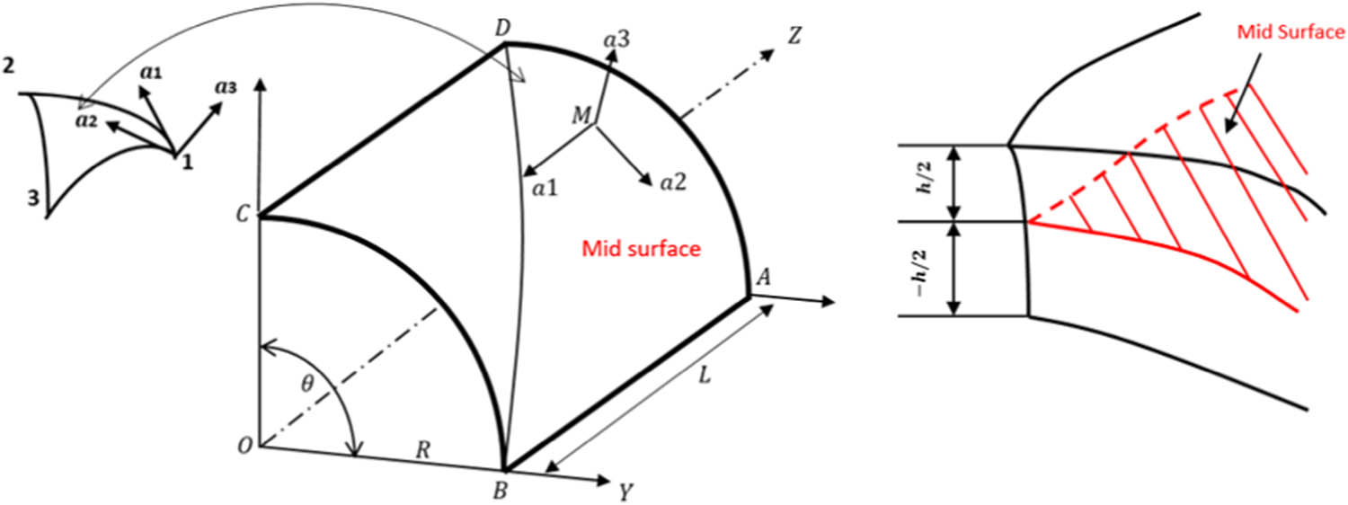
All existing formulations differ in the definition of the function f ( z ) used to represent transverse shearing. The Nzengwa and Tagne (N–T) two-dimensional model for linear elastic thick shells has been deduced from the three-dimensional problem without any ad hoc assumption whether of a geometrical or mechanical nature. The two-dimensional equations are deduced by applying asymptotic analysis on a family of variational equations obtained from an abstract scaled shell through multiple scaling of the initial three-dimensional equations.

The N–T shell model gives the following displacement results

In the basis ( G α , A 3 )
(3) U α ( x 1 , x 2 , z ) = u ¯ α − z ( u 3 , α − 2 b α λ u ¯ λ ) + z 2 ( b α λ b λ ρ u ¯ ρ + b α λ u 3 , λ ) , U 3 ( x 1 , x 2 , z ) = u ¯ 3 ( x 1 , x 2 ) .
In the basis ( A α , A 3 )

(4) U ¯ α ( x 1 , x 2 ) = ( μ α τ ) u τ − z ∂ α u 3 ; U ¯ 3 ( x 1 , x 2 ) = u 3 .

The strain tensor deduced from shells’ kinematics with respect to the plane strain state reads

(5) ε α β ( u ¯ ) = e α β ( u ¯ ) − z k α β ( u ¯ ) + z 2 Q α β ( u ¯ ) ,

(6) ε i 3 = 0 ,

(7) e α β ( u ¯ ) = 1 2 ( ∇ α u ¯ β + ∇ β u ¯ α − 2 b α β u 3 ) ,

(8) k α β ( u ¯ ) = ∇ α b β υ u ¯ υ + b α υ ∇ β u ¯ υ + b β υ ∇ α u ¯ υ + ∇ α ∇ β u ¯ 3 − b α ρ b β ρ u ¯ 3 ,

(9) Q α β ( u ¯ ) = 1 2 ( b α υ ∇ β b υ τ u ¯ τ + b α υ b υ τ ∇ β u ¯ τ + b β υ b υ τ ∇ α u ¯ τ + b β υ ∇ υ b α τ u ¯ τ + b α υ ∇ β ∇ υ u ¯ 3 + b β υ ∇ α ∇ υ u ¯ 3 ) .

We express the strain components using the parameters of the cylindrical shell’s midsurface. In detail, we have:

(10) e x x = u ¯ 1 , x ; e φ φ = 1 R ( u ¯ 2 , φ + u 3 ) ; 2 e x φ = 1 R u ¯ 1 , φ + u ¯ 2 , x ; k x x = u 3 , x x ; k φ φ = − 1 R 2 ( 2 u ¯ 2 , φ − u 3 , φ φ ) ; 2 k x φ = − 1 R ( u ¯ 2 , x − u 3 , x φ ) ; Q x x = 0 ; Q φ φ = − 1 R 3 ( u ¯ 2 , φ − u 3 , φ φ ) ; 2 Q x φ = − 1 R 2 ( u ¯ 2 , x − u 3 , x φ ) .

2.2 Hygral–mechanical finite element modeling

The approach used here is based on strain interpolation using curved shell finite elements (CSFE-sh) with shifted-Lagrange triangular element (Figure 1) with three degrees of freedom per node rather than five [26].

Figure 1

Triangular shell element.

The law of linearized hygral elastic behaviour written in the absence of internal bonds takes the same form as thermal formulation. Most stresses are mainly generated in circumferential (hoop) and radial directions because shrinkage in vertical directions is much less significant as compared to those in circumferential and radial directions [27]. For a shell Ω = S × ] − h / 2 , h / 2 [ , using the linearized constitutive law, the variational equation at the first order (see [24]) reads:

(11) ∫ Ω ( [ λ ¯ g α β g γ ρ + μ ( g α γ g β ρ + g α ρ g β γ ) ] ε α β ( u ¯ ) − α ¯ E Δ ω ) : ε α β ( v ) d Ω = L ( v ) .

with λ ¯ = 2 μ λ λ + 2 μ , Δ ω is the water gradient into the mixture, α ¯ is the shrinkage coefficient.

Eq. (11) is equivalent to

(12) ∫ S [ N ˜ ( u ¯ ( x ) ) : e ( v ) + M ( u ¯ ( x ) ) : k ( v ) + M ⁎ ( u ¯ ( x ) ) : Q ( v ) ] d s − ∫ Ω α ¯ E Δ ω : ε α β ( v ) d Ω = L ( v ) ,

where the functions of the bilinear form are expressed by

N ˜ = N + N ¯ , M ⁎ = M ¯ + M ¯ ¯ ;

(13) M ¯ α β E h 3 12 ( 1 − ν 2 ) [ ( 1 − ν ) e α β ( u ¯ ( x ) ) + v e ρ ρ ( u ¯ ( x ) ) A α β ] , M ¯ ¯ α β = E h 5 80 ( 1 − ν 2 ) [ ( 1 − ν ) Q α β ( u ¯ ( x ) ) + v Q ρ ρ ( u ¯ ( x ) ) A α β ] , N ¯ α β = E h 3 12 ( 1 − ν 2 ) [ ( 1 − ν ) Q α β ( u ¯ ( x ) ) + v Q ρ ρ ( u ¯ ( x ) ) A α β ] , M α β = E h 3 12 ( 1 − ν 2 ) [ ( 1 − ν ) k α β ( u ¯ ( x ) ) + v k ρ ρ ( u ¯ ( x ) ) A α β ] , N α β = E h 1 − ν 2 [ ( 1 − ν ) e α β ( u ¯ ( x ) ) + v e ρ ρ ( u ¯ ( x ) ) A α β ] .

3 Moisture transport problem at an early age

Structures based on cementitious materials see their initial water content decrease regardless of the environment in which they are placed. The anhydrous cement grains try to capture the water molecules to hydrate themselves, and during this time, a thermodynamic balance tries to be established with the external environment.

3.1 Bound water formulation

Onsite conditions, the cement-based materials are generally exposed to climatic conditions after casting at least upon one face. At the early age, Powers and Brownyard quoted by Brouwers [28] distinguish in the core of concrete free water, bound water, and water that cannot be evaporated which is neglected here. At time t, water contained in the material is the sum of free and bound water. Hydration law depends on the quantity of free water available in the mixture. We assume that just after casting (time t 0 ), the entire water contained in the material is free water. The water likely to be evaporated is free water which is mobilised for cement hydration. Let ω the total water content at time t ≠ t 0

(14) ω L = ω − ω h .

Eq. (14) is completely determined if bound water can be evaluated independently. It is known that the bound water is proportional to the quantity of cement in the mixture and the hydration degree. So, the bound water can be well approximated by the following relation:

(15) ω h = 0.23 B m ξ .

The explicit expression of free water is deduced from this

(16) ω L = ω − 0.23 B m ξ .

Hydration degree is expressed in the following rate form, where its dependence on temperature is described by the Arrhenius-type law

(17) d ξ d t = A ˜ ( ξ ) β h ω L ω 0 exp − E a R T ,

where A ˜ denotes the chemical affinity representing the driving force of hydration reaction, E a is the activation energy, R is the perfect gas constant, T is the ambient temperature, and β h a function deduced from the isotherm desorption curve of the concrete

(18) β h = 1 + a 1 − 2.0861 ω L ω 0 3 − 2.9132 ω L ω 0 2 + 1.8056 ω L ω 0 − 1 ,

with a to suppress the parameter taken equal to 3.5. We consider the chemical affinity A ˜ to be a quadratic function as defined in ref. [29]

(19) A ˜ ( ξ ) = γ 1 ( γ 2 + γ 3 ξ + ξ 2 ) ( ξ u − ξ ) exp − η ξ ξ u ,

where γ 1 , γ 2 , γ 3 , η are material coefficients and ξ u the ultimate hydration degree defines from water over cement (W/c) ratio by Mills’s relation

(20) ξ u = 1.031 W / c 0.194 + W / c .

3.2 Drying of concrete

Water contained in the core of the material can be in a liquid or gaseous phase. According to Daian [30], the water liquid flow and vapor water flow can be expressed with the same potential such that the free water takes the form

(21) ∂ ω L ∂ t = div ( D v ( ω L ) ∇ ω L ) .

Its variation is significant in the change of moisture transport due to drying [31,32]. Consequently, to model the diffusion phenomenon, the approach of Mensi et al. is considered [33]:

(22) D v ( ω L ) = A exp ( B ω L ) .

The parameter B can be taken as a constant, B = 0.05. The drying parameter A needs to be determined. We assume that water content variation in the medium is due to hydric transfer and hydration process. The boundaries conditions used are in the convective form

(23) h c = δ ( 2 ω 0 − ω f − ω L ) ,

where δ is the material coefficient which characterizes drying velocity. The convective coefficient denoted h c is a function of ω L . The normal flow at the face exposed can be written as follows:

(24) D v ( ω L ) ∂ ∇ ω L ∂ n ⋅ n = − δ ( 2 ω 0 − ω f − ω L ) ( ω L − ω f ) .

Using the finite element technic, the domain Ω is divided into elements. Let ω L ∈ C 0 ( Ω ¯ ) ⊂ H 1 ( Ω ) and v ∈ H 1 ( Ω ) .

The variational equation leads to

(25) ∫ Ω ∂ ω L ∂ t v d Ω = − ∫ Ω D v ( ω L ) ∇ ω L ∇ v d Ω − ∫ ∂ Ω δ ( 2 ω 0 − ω f − ω L ) ω L v d s + ∫ ∂ Ω δ ( 2 ω 0 − ω f − ω L ) ω f v d s .

The relation (25) is reorganized as follows:

(26) ∫ Ω ω ̇ L v d Ω + ∫ Ω D v ( ω L ) ∇ ω L ∇ v d Ω + ∫ ∂ Ω 2 δ ω 0 ω L v d s = ∫ ∂ Ω δ [ ( 2 ω 0 − ω f ) ω f + ω L . ω L ] v d s .

Eq. (26) is nonlinear. For y ∈ C 0 ( Ω ) , we pose y 0 = ω n and the Eq. (26) is linearized as follows:

(27) ∫ Ω ω n + 1 − ω n Δ t v d Ω + ∫ Ω D v ( y 0 ) ∇ ω L n + 1 ∇ v d Ω + ∫ ∂ Ω 2 δ ω 0 ω L n + 1 v d s = ∫ ∂ Ω δ [ ( 2 ω 0 − ω f ) ω f + y 0 ω L n + 1 ] v d s .

The Crank–Nicholson algorithm can also be used as done in ref. [34]. Eq. (27) can be easily resolved, and we obtain the first approximation of the solution denoted y 1 . To seek the real solution of Eq. (27), the following algorithm is established

(28) y 0 = ω n y n + 1 = y n − ρ ( y n − y n − 1 ) .

ρ ∈ [ 0 ; 1 ] . If Eq. (28) admits a solution, then the solution sought is ω L n + 1 = y n + 1 . In this study, one-dimensional analysis is sufficient for establishing the hydric profile across the depth.

4 Consideration of strains

It is important to state that the dimension variations recorded at each side are the total strain, which expresses the global response of the material to the various stresses induced by several phenomena such as shrinkage, creep and relaxation, and thermal effects which is neglected here depending to the position parameter ( x )

(29) ε ( x , t ) = ε e ( x , t ) + ε s h ( x , t ) + ε c r ( x , t ) + ε t h ( x , t ) ,

where ε e is the elastic strain, ε s h is the total shrinkage strain, ε c r represents creep strain, and ε t h the thermal strain.

The phenomenon of shrinkage is principally linked to the variation of water content in the material in laboratory conditions. In practice, it is sufficient to consider autogenous and drying shrinkage for concrete studies. As autogenous shrinkage is directly related to hydration, many models propose a relationship between shrinkage and hydration degree as indicated in Eq. (30) below

(30) ε ash ( x , t ) = κ Δ ω h ( x , t ) I .

I is the identity matrix and Δ ω h the gradient of bound water. The loss of moisture during drying results in a contraction of the cement paste as shown in Eq. (31)

(31) ε d s h ( x , t ) = p ω e ( x , t ) .

ω e is the evaporable water. We assume that total shrinkage is the sum of drying and autogenous shrinkage

(32) ε s h ( x , t ) = ε a s h ( x , t ) + ε d s h ( x , t ) .

The quantity α ¯ Δ ω expressed in Eq. (11) can be written as

(33) α ¯ Δ ω ( x , t ) = ( κ Δ ω h ( x , t ) + p ω e ( x , t ) ) .

Young’s modulus is expressed here as a function of hydration degree according to De Schutter and Taerwe [35]

(34) E ( x , ξ ) = ξ − ξ 0 1 − ξ 0 b × E ( x , ξ = 1 ) .

The constant b and the modulus at the ultimate hydration degree have to be known. ξ 0 is the minimal hydration degree corresponding to the threshold percolation taken equal to 0.25 for ordinary Portland cement. We retain the constant defined by Zreiki et al. [36] in their works on concrete ξ 0 = 0.223 and b = 0.25. The stress developed in the concrete mass induces a displacement of the structure and is therefore equivalent to a surface loading on the different layers. The hydration field linked by the moisture gradients over the thickness of the material has an influence on the evolution of Young's modulus at each point taken over the thickness and consequently stresses. Subsequently, the creep develops and relaxes the stresses in the material due to the prestress undergone by the ring when it is submitted to drying. Thus, the response of material can be predicted by using an established model for predicting creep and strain relaxation phenomenon from ring test [37]

(35) E c a ( x , ξ , t 0 , t ) = E ( x , ξ ) 1 + ψ ( x , t 0 , t ) ⋅ ϕ ( t 0 , t ) ,

where E ( x , ξ ) is the short-term elastic modulus at time t at location x, t ₀ is the age (in days) when the shrinkage load (or deformation) is applied, ϕ ( t 0 , t ) is the creep coefficient defined by a creep strain under constant stress in time t divided by initial elastic strain in time t ₀, ψ ( x , t 0 , t ) is the ageing coefficient which is expressed as follows:

(36) ψ ( x , t 0 , t ) = 1 − E R ( x , t 0 , t ) E ( x , t 0 ) − 1 − 1 ϕ ( t 0 , t ) .

E R ( x , t 0 , t ) and E ( x , t 0 ) are the relaxation function that can be determined from Volterra’s integral equation as follows:

(37) J c ( t 0 , t ) ⋅ E ( x , t 0 ) + ∫ t 0 + t J c ( t ' , t ) ∂ E R ( x , t 0 , t ' ) ∂ t ' d t ' = 1 .

With J c ( t ' , t ) = [ 1 + ϕ ( t ' , t ) ] / E ( x , t ' ) the creep function, and E ( x , t ' ) is the time-dependent Young’s modulus at location x .

To determine the tensile creep coefficient, recent work has described an approach based on the use of strain measured from the shrinkage test, as specified in the standard NF P 15-433, with those measured from the restrained ring test following ASTM C1581 [38].

Therefore, the creep coefficient can be calculated as follows:

(38) ϕ ( t 0 , t ) = ε c p ( t ) ε e ( t ) = E c ( t ) ⋅ r i s ⋅ h c E s t ( t ) ⋅ r i c ⋅ h s t ε s h ( t ) ε s t ( t ) − 1 − 1 ,

where ε s h ( t ) is the free shrinkage measured on 7 cm × 7 cm × 28 cm prismatic samples according to NF P 15-433 specification, E c ( t ) is the elastic modulus of the concrete ring depending of time, E s t ( t ) is the elastic modulus of the steel ring considered to be constant, h c is the concrete ring thickness, h s t is the steel ring thickness, r i c is the inner radius of concrete ring, r i s is the inner radius of steel ring, and ε e ( t ) is the elastic strains developed on the concrete ring.

The strain linked to the loss of water by evaporation increases with time and the self-stresses generated will undergo a reduction due to the relaxation.

Based on the deformation continuity principle between the two rings [39], the elastic strains of the concrete ring can be determined from steel strains development as follows:

(39) ε e ( t ) ⋅ E c ( t ) = E s i ⋅ r i c ⋅ h s t r i s ⋅ h c ε s t ( t ) ,

where ε c p ( t ) is the creep strains developed on the steel ring and ε s t ( t ) is the total strain measured on the steel ring.

We assume that the visco-elastic parameter ψ is as constant in the thickness and took equal to 0.57. Therefore, the parameter ϕ becomes the only parameter to be calculated. The variations in time of strains measured with ring test and free shrinkage test are plotted in Figure 2.

Figure 2

Variations in time of strains measured from ring specimens and 7 cm × 7 cm × 28 cm prismatic samples.

The variations in the time of creep coefficient calculated are given in Table 1.

Table 1

Creep coefficient variations

	1 Day	3 Days	7 Days	28 Days
Creep coefficient ϕ(t0, t)	0.18	0.91	1.02	1.2

5 Main data of tested shell

In this work, two thick cylindrical specimens (Figures 3 and 4) of unreinforced concrete were cast, instrumented, and subjected to drying in laboratory conditions (temperature, 22°C ± 1; relative humidity, 70 ± 5%). The shell is cylindrical, with an internal radius of R ₁ = 37.5 cm and an external radius of R ₂ = 47.5 cm. The ratio thickness over the smallest radius in absolute value is equal to χ = h / R min = 0.26 where h = 10 cm.

Figure 3

Geometry details of the test specimen.

Figure 4

Sample preparation and instrumentation.

5.1 Concrete mix

The cement used in this study is an ordinary Portland cement CEM I 42.5 N. The uniaxial compressive strength of concrete was determined on the cubic specimen of 10 cm side at 28 days. The mix proportions and the average compressive strength ( f c ) are presented below (Table 2).

Table 2

Composition of concrete

Composition of concrete
Water (W)	Cement (c)	Sand (s)	Gravel 0/15	W/c	fc
216 l	400 kg	800 l	965 l	0.54	20 MPa

5.2 Mass loss and free shrinkage measurement

For shrinkage and mass loss measurement, concrete specimens of the size of 7 cm × 7 cm × 28 cm and other prisms specimens of the size of 10 cm × 10 cm × 10 cm were cast. The measurements of shrinkage were started after form removal (24 hours after casting); then, the specimens were placed in the controlled room. Autogenous shrinkage was measured on three specimens of the size of 7 cm × 7 cm × 28 cm sealed with an adiabatic waterproof sheet to prevent drying. Also, the 10 cm × 10 cm × 10 cm prisms used for monitoring the mass loss are sealed with waterproof paint, and only one side is left free for drying.

5.3 Rings specimens preparation and instrumentation

The ring specimens were demoulded 24 hours after pouring. After that period, the waterproof paint is applied to the inner and top faces of the ring, and then, the whole is covered with the polyan sheet for 22 hours.

The instrumented ring specimens, data acquisition system and steel molds used are shown in Figure 4. We considered:

The micrometer-sensitive digital comparators for displacement measurement. To monitor the displacements, the comparators are placed at different points of its thickness along the x-axis from the centre of the ring, respectively, at 39 cm (C₃), 42.5 cm (C₂), and 46 cm (C₁);
The strain gauges are bonded in the both inner face and outer face of the rings 22 hours after steel form removal. The adhesive used consists of a two-component “M-Bond AE-15 Kit for strain gages” proposed by MICRO MEASUREMENTS. This adhesive is highly resistant to moisture. For strains recovering, the strain gauges are fixed along the hoop direction of the rings;
A data acquisition system in a quarter-bridge configuration for strain recording;
A plastic film was placed below to prevent any suction of water from the test piece through the substrate and allow a free displacement at the base of the specimen.

After preparation and instrumentation, the rings were exposed to drying after the removal of the plastic film. This corresponds to a cured period of 48 hours after casting.

6 Results and discussion

Experimental campaign was carried out for several days then, and the collected data were stripped and analyzed. The water contraction coefficients and the percentage of mass loss recorded on the samples were therefore be calculated.

Figure 5

Exchange coefficient.

Figure 6

Diffusion coefficient.

6.1 Fitting drying parameters

Based on the results of mass loss measurements, the diffusion coefficient is defined by parameter A = 2.356 × 10 − 13 , and we used δ = 2.242 × 10 − 11 to consider the exchange with the environment (Figures 5 and 6). The material coefficients used for chemical affinity are respectively γ 1 = 1.102 × 10 − 7 , γ 2 = 0.0065 , γ 3 = − 0.145 , and η = 7.95 . The numerical simulation of drying has been done. After several days of exposition, moisture content decreases in the material. As can be seen in Figure 7, the evaporable water can be correlated with the mass loss with higher kinetic. This kinetic attenuates and slowly grows until the water balance is reached Figure 8.

Figure 7

Mass loss.

Figure 8

Free water evolution at different points.

6.2 Evolution of water content in time and the thickness

The trend of water moisture evolution (Figure 9) according to time shows that free water variation tends asymptomatically towards the water content of the environment. The evolution of the free water content in the thickness is shown in Figure 10. Globally, the non-uniform moisture distribution is observed. The internal moisture differs significantly according to the depth from the exposed surface where the free water content is small as compared to the rest of the thickness. It appears that the drying kinetics is much accentuated for the outer sheet while the inner sheets are substantially slow.

Figure 9

Mean water variation in the mixture.

Figure 10

Water variation in the cross section.

The internal moisture differs significantly according to the depth from the exposed surface where the gradients of free water content are greater compared to the rest of the thickness.

Young’s modulus of the material is linked to the degree of hydration and varies according to the position considered as a function of the water content. We note a low variability of the modulus in the thickness (Figure 11) with a maximum coefficient of variation estimated at 0.4% at 4 days (Figure 12).

Figure 11

Young modulus variation in the thickness at different age.

Figure 12

Young modulus coefficient of variation.

The result of radial displacement simulated at the midsurface is presented in Figure 13. We can observe that both measured displacement and those simulated evolve in the same way with the sample amplitude and similar kinetic evolution. The displacement model result is compared to the displacement measured on the midsurface, and the observed value difference may be due to the complex behaviour of the concrete ring at a young age. The shell theoretical model used in this study is unable to compute transverse strains through thickness.

Figure 13

Midsurface displacement.

6.3 Displacements and strains evolution

The mechanisms allowing the development of the shrinkage generate deformations which also result in a measurable displacement using the sensors placed on the thickness of the benchmark. We are interested here in the displacements in the hoop direction, and we neglect the displacement along the generatrix.

6.3.1 Displacement’s measurement in time and the thickness

The results of radial displacements are given in Figure 14. The results show that the radial displacement near the exposed surface is greater as compared to those measured near the inner face and midsurface. At the same time, the radial displacement measured near the inner surface is lower than the two others and can be considered practically constant. Also, the increase of displacements is globally observed at the half outer layer of the ring. This confirms the fact that the shell is the seat of the stress field induced by the restrained shrinkage phenomenon occurring in drying conditions. The gradients of displacements are also observed from the outer surface to the inner surface.

Figure 14

Measured radial displacements (μm).

6.3.2 Strains measurement in time and the thickness

Because the shell is the seat of a stress field-induced par shrinkage phenomenon, strains then develop in the core of the material. The total strains measured express the global response of the material to the various stresses induced by shrinkage, creep and relaxation effects. The evolution of strains measured on benchmark 1 at the outer and inner surfaces is presented in Figure 15. It should also be noted that the external deformation measurement gauge (DataR2ext) on ring 2 ceased to operate after approximately five days. The problem is believed to be related to the connection of said gauge.

Figure 15

435 Measured strains (μm/m).

We can observe that in the first days of drying, both sides of the specimen deform in the same way with the same amplitude of deformations and the same kinetic evolution. Then, a second time, the strains measured at the outer face begin to decrease and end by changing the sign while at the same time the increase of the strains measured at the inner face is observed. This evolution of strain development in the thickness can be attributed to the tensile creep phenomenon and its relaxation effects which are responsible for the release of stress observed on the thickness. Afterwards, we assume that, the drying kinetics being different from one side to the other, the movements of the exposed layers are restricted by the interior layers. This situation leads to the development of tensile creep the stress being kept constant by step period in time. These tensile stresses can lead to damage in severe conditions.

6.4 Simulation of strains evolution

In order to simulate the deformations of the structure linked to shrinkage, it is essential to determine the water contraction coefficients from the shrinkage measurements recorded on the prismatic specimens.

6.4.1 Fitting shrinkage parameters

For the determination of hydric contraction coefficients, the autogenous and drying shrinkage was recorded to the loss of mass measured on 7 cm × 7 cm × 28 cm prismatic samples. We retain both the values of k = 2.47 × 10 − 6 and p = 3.6 × 10 − 6 , respectively, reliable to length changes at self-desiccation and drying conditions.

6.4.2 Modeling strains evolution in time and depth

The results of the total strains simulated are the superposition of shrinkage and creep effects. We can observe that in the first days after demolding, both measured strains and simulated strains evolve in the same way with the same amplitude and same kinetic evolution (Figure 16). These strains can be considered as being generated mainly by the shrinkage linked to the change of internal moisture in the material, including hydration. Then, a second time, the strains measured decrease greatly with the change in the kinetic. In this case, shrinkage is greater at the outer surface exposed to drying compared to the rest of the thickness. The displacement of the outer layers due to differential shrinkage compresses the inner layer, and as the displacement of the inner layer is restrained by the geometrical shape of the specimen, this last one will bring the outer layer in tension. This tendency can be explained by the fact that the change in measured strain kinetics can be related to rapid development of creep and stress relaxation the material undergoes.

Figure 16

Total strains versus time without relaxation effect.

Looking carefully at the displacements and strains recorded, everything happens as if the inner layers of the specimen behaved like successive rings with differences in mechanical properties. The strains gradually increase with time as the inner layer cannot deform freely; this leads to the adaptation of material, and there is therefore a relaxation of the stresses. This can probably explain the change in the kinetics of the strains observed for the inner layer.

It can be observed that the tensile creep consideration would just decrease the amplitude of strains. Strain is caused by the departure of the water, and the shape of the strains is similar to the evolution of free water along the thickness.

Figure 17 represents hoop strain distribution along thickness at 14 days. Gradients of strains along the thickness follow the same evolution as the free water gradient in the material thickness.

Figure 17

Hoop strain distribution along the thickness.

The hoop stress that develops in the material is not harmful to compression loading but reaches about 2 MPa at 14 days (Figure 18).

Figure 18

Hoop stress along the thickness.

7 Conclusion

In this framework, stress analysis is performed on a simple thick-walled cylinder subjected only to the effect of natural drying. An experimental campaign on cylindrical specimen and numerical simulation was conducted. A hydro-mechanical formulation has been employed to obtain the midsurface displacement using water gradient by analogy with thermal expansion. An attempt has been made to determine strain evolution in the core of material using two-dimensional (2D) thick shell theory. The simulation done showed that the hydration degree is a function of the considered location on the thickness and thus, the related Young’s modulus. However, when the thickness tested is low, the variation in modulus is negligible. With regard to strains, strain law variation along the thickness is led by the water gradient which depends on drying boundary conditions. Consequently, the gradients of strains related to the water content can develop. The strains gradually increase with time as the inner layer cannot deform freely; this leads to the adaptation of material and therefore relaxation of the stresses.

For ring specimens, the outer layers located near the drying face are rapidly subjected to the tension resulting from the interaction with the internal layers; consequently, the specificities of the ring’s test are globally reproduced without the use of the brass ring. The curve of the strain evolution recorded on the outer sheet is similar to that of a part subjected to tensile creep as reported by Ranaivomanana et al. [40]. At the same time, the inner members are globally compressed, assuming that the specimen undergoes prestressed.

At last, as the fluctuations of the strain's kinetics would result from the adjustment of the material due to the stress relaxation, this phenomenon can be taken in the simulation to attenuate evolution and changes of kinetic strains on the concrete ring. Therefore, the effects of creep deserve to be studied more because existing models do not approach enough the deformations of the ring.

Acknowledgement

The authors would like to thank the research team of the Civil Engineering laboratory of SJP- Polytechnic Institute of Douala as well as that of the L2MGC laboratory of CY-Cergy Paris University for providing necessary equipment for data acquisition during the course of this research. Our special thanks go to the following people: Prof. Albert Noumowé; Prof. Anne-Lise Beaucour; Prof. Javad Elsami; Msc Steve M. Nkomom; Msc. Hugues S. Taowe

Funding information: The authors state no funding involved.
Conflict of interest: Authors state no conflict of interest.
Data availability statement: Measurement data is available to anyone who wants it.

References

[1] Radnić J, Matešan D. Testing of prestressed concrete shell under long-term load and unload. Exp Mech. 2009;50:575–88.10.1007/s11340-009-9242-9Search in Google Scholar

[2] Torrenti JM, Benboudjema F, Chauvel D, Barré F. Retrait de dessiccation des bétons: résultats du PN CEOS.fr, 31emes rencontres de l'AUGC. ENS Cachan; 2013.Search in Google Scholar

[3] Duprat F, Sellier A. Fiabilité des ponts en béton précontraint soumis au fluage, 19ème Congrès Français de Mécanique; 2009 Aug 24–28; Marseille, France.Search in Google Scholar

[4] Bažant ZP, Jirásek M. Creep and hygrothermal effects in concrete structures. Solid Mech its Appl. 2018;225:960.10.1007/978-94-024-1138-6Search in Google Scholar

[5] Halicka A, Podgórski J. Designing of cylindrical concrete tanks with regard to buckling and second order effects. Procedia Eng. 2017;193:50–7.10.1016/j.proeng.2017.06.185Search in Google Scholar

[6] Miyazaki N, Hagihara S. Creep buckling of shell structures. Mech Eng Rev. 2015;2(2):14-00522.10.1299/mer.14-00522Search in Google Scholar

[7] Duissenbekov B, Tokmuratov A, Zhangabay N, Orazbayev Z, Yerimbetov B, Aldirayov Z. Finite-difference equations of quasistatic motion of the shallow concrete shells in nonlinear setting. Curved Layer Struct. 2020;7:48–55.10.1515/cls-2020-0005Search in Google Scholar

[8] Chepurnenko A, Mailyan L, Yazyev B, Ivanov A. Calculation of the rotation shells on axisymmetric load taking the creep into account. MATEC Web Conf. 2017;106:04011.10.1051/matecconf/201710604011Search in Google Scholar

[9] Andreev V, Cherpurnenko A, Yazyev B. Calculation of creep of circular cylindrical shell by bending theory. Procedia Eng. 2016;165:1141–6.10.1016/j.proeng.2016.11.831Search in Google Scholar

[10] Karpov V, Semenov A. Computer modeling of the creep process in stiffened shells. International Scientific Conference Energy Management of Municipal facilities and Substaiable Energy Technologies EMMFT. vol. 1, 2018. p. 48–58.10.1007/978-3-030-19756-8_5Search in Google Scholar

[11] Hamed E, Bradford MA, Gilbert RI. Nonlinear long-term behaviour of spherical shallow thin-walled concrete shells of revolution. Int J Solids Struct. 2010;47:204–15.10.1016/j.ijsolstr.2009.09.027Search in Google Scholar

[12] Wang X, Sun B, Li S, Wang Z, Li H, Gao Y, et al. Numerical modeling of hydration performance for well cement exposed to a wide range of temperature and pressure. Constr Build Mater. 2020;261:119929.10.1016/j.conbuildmat.2020.119929Search in Google Scholar

[13] Zhang L, Qian X, Lai J, Qian K, Fang M. Effect of different wind speeds and sealed curing time on early-age shrinkage of cement paste. Constr Build Mater. 2020;255:119366.10.1016/j.conbuildmat.2020.119366Search in Google Scholar

[14] Khan I, Castel A, Xu T, Ian Gilbert R. Early-age tensile creep and shrinkage induced cracking in internally restrained concrete members. Mag Concr Res. 2018;71(22):1167–79.10.1680/jmacr.18.00038Search in Google Scholar

[15] Amba JC, Balayssac JP, Détriché CH. Characterization of differential shrinkage of bonded mortar overlays subjected to drying. Mater Struct. 2010;43:297–308.10.1617/s11527-009-9489-8Search in Google Scholar

[16] Goh CY, Hrynyk TD. Nonlinear finite element analysis of reinforced concrete flat plate punching using a thick-shell modelling approach. Eng Struct. 2020;224:111250.10.1016/j.engstruct.2020.111250Search in Google Scholar

[17] Lin J, Naceur H, Laksimi A, Coutellier D. Modélisation de structures minces de type coques en comportement non linéaire géométrique par la méthode SPH, 21e Congrès français de mécanique; 2013 Aug 26–30; Bordeaux, France.Search in Google Scholar

[18] Fantuzzi N, Tornabene F, Viola E. Generalized differential quadrature finite element method for vibration analysis of arbitrarily shaped membranes. Int J Mech Sci. 2014;79:216–51.10.1016/j.ijmecsci.2013.12.008Search in Google Scholar

[19] Tornabene F, Viscoti M, Dimitri R. Equivalent single layer higher order theory based on a week formulation for the dynamic analysis of anisotropic doubly-curved shells with an arbitrary geometry and variable thickness. Thin-Walled Struct. 2022;174:109119.10.1016/j.tws.2022.109119Search in Google Scholar

[20] Tornabene F, Viscoti M, Dimitri R, Aiello MA. Higher order formulations for doubly-curved shell structures with a honeycomb core. Thin-Walled Struct. 2021;164:1107789.10.1016/j.tws.2021.107789Search in Google Scholar

[21] Tornabene F, Viscoti M, Dimitri R. Generalized higher order layerwise theory for the dynamic study of anisotropic doubly-curved shells with a mapped geometry. Eng Anal Bound Elem. 2022;134:147–83.10.1016/j.enganabound.2021.09.017Search in Google Scholar

[22] Gallegos-Cazares S, Schnobrich W. Effect of creep and shrinkage on the behavior of reinforced concrete gable roof hyperbolic-paraboloids. Civil Engineering Studies: Structural Research Series No. 543. University of Illinois; 1988.Search in Google Scholar

[23] Luu CH, Mo YL, Hsu TTC. Development of CSMM-based shell element for reinforced concrete structures. Enginering Struct. 2017;132:778–90.10.1016/j.engstruct.2016.11.064Search in Google Scholar

[24] Nzengwa R, Tagne Simo BH. A two-dimensional model for linear elastic thick shells. Int J Solids Struct. 1999;36:5141–76.10.1016/S0020-7683(98)00165-6Search in Google Scholar

[25] Anyi JN, Nzengwa R, Amba JC, Ngayihi Abbe CV. Approximation of linear elastic shells by curved triangular finite elements based on elastic thick shells theory. Math Probl Eng. 2016;2016:8936075.10.1155/2016/8936075Search in Google Scholar

[26] Anyi JN, Amba JC, Essola D, Ngahiyi Abbe CV, Bodol Momha M, Nzengwa R. Generalised assumed strain curved shell finite elements (CSFE-sh) with shifted-Lagrange and applications on N-T's shells theory. Curved Layer Struct. 2020;7:125–38.10.1515/cls-2020-0010Search in Google Scholar

[27] Wang S. Thermal analysis of cylindrical concrete shell at transition boundary between regions with different reinforcement configurations. Eng Struct. 2015;84:279–86.10.1016/j.engstruct.2014.11.038Search in Google Scholar

[28] Brouwers HJH. The work of powers and brownyard revisited: Part 1. Cem Concr Res. 2004;34(9):1697–716.10.1016/j.cemconres.2004.05.031Search in Google Scholar

[29] Zheng Z, Wei X. Mesoscopic models and numerical simulations of the temperature field and hydration degree in early-age concrete. Constr Build Mater. 2021;266:121001.10.1016/j.conbuildmat.2020.121001Search in Google Scholar

[30] Daian J-F. Condensation and isothermal water transfert in cement mortar: Part I. Transp Porous Media. 1988;13:563–89.10.1007/BF00959103Search in Google Scholar

[31] Zhang J, Hou D, Gao Y, Wei S. Determination of moisture diffusion coefficient of concrete at early age from interior humidity measurements. Dry Technology: An Int J. 2011;29(6):689–96.10.1080/07373937.2010.528106Search in Google Scholar

[32] Suwito A, Ababneh A, Xi Y, William K. The coupling effect of drying shrinkage and moisture diffusion in concrete. Comput Concr. 2006;3(2):103–22.10.12989/cac.2006.3.2_3.103Search in Google Scholar

[33] Mensi R, Acker P, Attoulou A. Séchage du béton: analyse et modélisation. Mater Struct. 1988;21:3–12.10.1007/BF02472523Search in Google Scholar

[34] Babaei M, Kiarasi F, Asemi K, Dimitri R, Tornabene F. , Transient thermal stresses in FG porous rotating truncated cones reinforced by graphene platelets. Appl Sci. 2022;12:13932.10.3390/app12083932Search in Google Scholar

[35] De Schutter G, Taerwe L. Degree of hydration-based description of mechanical properties of early age concrete. Mater Struct. 1996;29:335–44.10.1007/BF02486341Search in Google Scholar

[36] Zreiki J, Lamour V, Moranville M, Chaouche M. Détermination des contraintes mécaniques dans les pièces massives en béton au jeune âge: instrumentation in-situ et modélisation, 8eme édition des journées scientifiques du regroupement francophone pour la recherche et la formation sur le béton (RF) B; 2007. p. 2.Search in Google Scholar

[37] Pedro Alex Sanchez Hernandez, Prediction of Creep, Shrinkage, and Temperature Effects in concrete structures. Farmington Hills (MI): ACI Committee; 1997. p. 209.Search in Google Scholar

[38] Nguyen T-H. Durabilité des réparations à base cimentaire: analyse compare de l’influence des propriétés mécaniques du matériau de réparation [dissertation]. Toulouse: Université Tolouse-III- Paul Sabatier; 2010.Search in Google Scholar

[39] Weiss WJ. Prediction of early age shrinkage cracking in concrete [dissertation]. Evanston (IL): Northwestern University; 1999.Search in Google Scholar

[40] Ranaivomanana N, Multon S, Turatsinze A. Basic creep of concrete under compression, tension and bending. Constr Build Mater. 2013;38:173–80.10.1016/j.conbuildmat.2012.08.024Search in Google Scholar

Received: 2022-05-05

Revised: 2022-07-22

Accepted: 2022-08-26

Published Online: 2023-01-21

This work is licensed under the Creative Commons Attribution 4.0 International License.

Articles in the same Issue

https://doi.org/10.1515/cls-2022-0179

Keywords for this article

shell; moisture; differential shrinkage; tensile creep; modeling

Creative Commons

BY 4.0