A novel approach for protein secondary structure prediction using encoder–decoder with attention mechanism model

Pravinkumar M. Sonsare; Chellamuthu Gunavathi

doi:10.1515/bmc-2022-0043

Article Open Access

A novel approach for protein secondary structure prediction using encoder–decoder with attention mechanism model

Pravinkumar M. Sonsare and Chellamuthu Gunavathi

Published/Copyright: March 13, 2024

Published by

Become an author with De Gruyter Brill

Submit Manuscript Author Information Explore this Subject

From the journal Biomolecular Concepts Volume 15 Issue 1

Abstract

Computational biology faces many challenges like protein secondary structure prediction (PSS), prediction of solvent accessibility, etc. In this work, we addressed PSS prediction. PSS is based on sequence-structure mapping and interaction among amino acid residues. We proposed an encoder–decoder with an attention mechanism model, which considers the mapping of sequence structure and interaction among residues. The attention mechanism is used to select prominent features from amino acid residues. The proposed model is trained on CB513 and CullPDB open datasets using the Nvidia DGX system. We have tested our proposed method for Q ₃ and Q ₈ accuracy, segment of overlap, and Mathew correlation coefficient. We achieved 70.63 and 78.93% Q ₃ and Q ₈ accuracy, respectively, on the CullPDB dataset whereas 79.8 and 77.13% Q ₃ and Q ₈ accuracy on the CB513 dataset. We observed improvement in SOV up to 80.29 and 91.3% on CullPDB and CB513 datasets. We achieved the results using our proposed model in very few epochs, which is better than the state-of-the-art methods.

Keywords: bioinformatics; machine learning; deep learning; protein secondary structure prediction

Introduction

Scientists are working together with computer scientists to analyze the structure of a protein using techniques such as computational analysis. Proteins are composed of 20 amino acids. There are four types of structures that are commonly used in protein production. The primary, secondary, tertiary, and quaternary structures are the main types of protein structures. The primary structure of a protein refers to the linear sequence of amino acids in a polypeptide chain. It is determined by the order and type of amino acids linked together by peptide bonds. The primary structure is the most fundamental level of protein structure and is crucial for understanding the subsequent levels. Secondary structure refers to the local folding patterns within a polypeptide chain. Tertiary structure is the three-dimensional arrangement of the entire polypeptide chain including its secondary structures. It results from the interactions between amino acid side chains including hydrogen bonds, disulfide bonds, hydrophobic interactions, and van der Waals forces. The tertiary structure is critical for a protein’s overall shape and function [1,2]. Quaternary structure refers to the arrangement of multiple polypeptide chains (subunits) into a functional protein complex. Proteins with quaternary structure consist of two or more interacting polypeptide chains called subunits. The interactions between subunits involve the same types of forces that stabilize the tertiary structure.

Unfortunately, current methods for making predictions are time-consuming. Unfortunately, the current method could not address the real-world issue of measuring the percentage of amino acids in different forms or shapes of a protein [3,4,5]. An accurate prediction of the protein’s tertiary structure is also essential to determine its function. In this study, we developed a deep learning algorithm that can analyze the secondary structure of protein sequences. It can also predict the structure of the protein’s tertiary structures.

Deep learning techniques, especially neural networks, have become the dominant approach in protein secondary structure prediction. Convolutional neural networks (CNNs), recurrent neural networks (RNNs), and transformer-based models have shown significant improvements in accuracy. Transfer learning where models are pre-trained on large datasets and fine-tuned for specific tasks has gained popularity. Pre-training on related tasks such as language modeling has shown to enhance the performance of protein structure prediction models. Methods that leverage evolutionary information such as position-specific scoring matrices (PSSMs) derived from multiple sequence alignments have been integrated into prediction models. This allows models to capture evolutionary conserved features. Hybrid models combining different types of neural network layers such as combining CNNs with RNNs have been explored to capture both local and global features in protein sequences. The availability of larger and more diverse datasets has facilitated the training of more accurate models. Efforts have been made to develop real-time prediction tools that can rapidly predict protein secondary structures. This is important for applications such as drug discovery and structural bioinformatics.

Scientists use different computer methods to figure out how amino acids are arranged in a protein. It’s like solving a puzzle. They use techniques such as clustering, support vector machines (SVMs), random forests, and RNNs. Deep learning, which is a type of advanced computer learning, is also used to check how well we can predict the structure of proteins. Scientists use a special computer method called the K-nearest neighbor to describe the sequence of amino acids in a protein. It helps them understand the patterns and relationships in the sequence [6].

The SVM classifier is developed using PSSMs. SVM is combined with the jury decision system to generate a classification [7]. Machine learning techniques separate a globular protein into membrane protein [8]. Various probabilistic approaches are also used to predict its structure [9]. The folding shape is identified by proper PSS prediction. A Fourier technique is also used to predict the percentage of residues in a protein [10]. The random forest method is also used to generate a classification for an unknown protein [11]. This method is combined with the classification-based association algorithm to predict its structure [12].

Position-specific iterative basic local alignment search tool is a computational tool that allows developers to create a position-specific scoring matrix. It is used for input in a deep neural network architecture [13].

Convolutional layers are employed to capture the local patterns and dependencies in the protein sequence. Filters (kernels) slide across the input sequence, learning hierarchical features at different levels of abstraction. These features may represent the relevant motifs or patterns associated with secondary structure elements. Stacking multiple convolutional layers enables the network to learn increasingly complex and abstract representations of the input sequence. This hierarchical learning is essential for capturing the hierarchical structure of proteins. After convolutional layers, the feature maps are typically flattened and fed into fully connected layers. These layers integrate the information from different parts of the input sequence and provide the final prediction. Proteins are composed of amino acids arranged in a specific sequence. The RNN with their ability to capture sequential dependencies is well-suited for learning patterns and relationships within these sequences.

Neural network-based five models (feed forward neural network, learning vector quantization, probabilistic neural network, CNN, and CNN fine tuning) are used to predict PSS after it has been composed of residues components [14]. RNN is used for sequence data, while the long-term memory cell is used for the recurrent neural system. The bidirectional method in which input is passed both ways predicts the PSS [3]. A supervised deep model is used to perform the sampling and scaling of the conditional mark distribution [15]. Various machine-learning components are then used to classify the data collected from sequential data [16]. The deep neural network architecture is composed of feature extractors, which are used to predict the secondary structure of a protein. The complex and straightforward relationship between the structure and sequence of the protein is maintained [17].

A CNN is a method to capture the residues. It uses a bidirectional recurrent unit to capture the global sequence feature [18]. Multi-hyperplane classification is a method to predict the structure of the protein. It considers sample points near the hyperplane for training [19]. The RNN is an algorithm used for structure prediction. It combines the deep learning capabilities of an encoder–decoder (Enc–Dec) with the recurrent architecture of a network [5]. Reciprocal and bidirectional multiple layers RNN can extract information from the residues [20]. A cascaded network of CNN and a bidirectional RNN is used to predict the PSS [21–23].

Protein secondary structures have been identified as the links in the physical processes of primary sequences, typically random coils, folding into functional tertiary structures. An efficient protein secondary structure predictor was important especially when high-resolution experiments do not solve the structure of an amino acid sequence fragment. A reductive deep learning model called multi-layer perceptron RNN has been proposed to predict either 3-state or 8-state protein secondary structures. Two sorts of characteristics are generated using the query protein’s PSSM. The first feature includes fuzzy class memberships for each residue in the three secondary structure classes. The normalized PSSM feature set was the second feature set. The features are converted into vectors appropriate for neural network training using a sliding-window method with a window length of W. In convolutional neural network with a highway (CNN-H), any two neighboring convolutional layers share a highway that transports information from the current layer to the output of the next one which allows local contexts to be maintained. Lower layers extract local context and higher layers extract long-range interdependencies which allows for efficient protein secondary structure prediction. CNN-H not only uses fewer computer resources but also performs better in terms of prediction.

We have used the attention mechanism with Enc–Dec, which allows models to focus on specific parts of the input sequence. This has been integrated into protein secondary structure prediction models. This has improved the ability of models to capture long-range dependencies in amino acid sequences. We have designed a model with a COCOB optimizer to solve the sequence learning problem. We focus on the dependency between a variable number of inputs for dealing with amino acid residues.

This article is organized into seven sections. Preliminary Section presents a glimpse of deep learning architecture. In Proposed methodology Section, the proposed models are explained. Proposed methodology and Data preparation and experimental setup Sections present data preparation and experiment details. Results and Discussion Sections present the result of the proposed model and a comparison with the existing model. Conclusion and future work Section draws conclusions and future work.

Preliminary

Sequence learning problem

The length of amino acid sequence from which the protein secondary structure is predicted is not fixed. Protein secondary structure depends on the order of amino acids that appeared in the chain. The input size is not fixed in protein secondary structure prediction where residues are dependent on each other. Each input is dependent on previous and future inputs. This sequence learning problem cannot be solved by a feed-forward neural network and CNN efficiently.

Recurrent neural networks

The number of residues from which we predict a particular protein structure is unknown. The output at each time step depends on the input given at that time step. The traditional approach may require an exact number of output functions as input length. The solution is to use RNN for handling sequence problems which are shown in Figure 1. Recurrent connections between each time steps address the problem of dependent input.

Figure 1

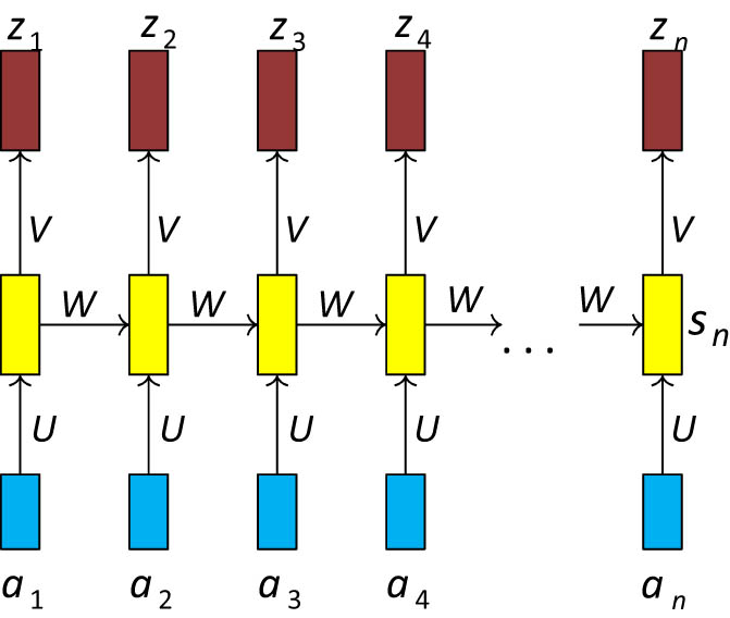
Recurrent neural network.

State of the network s t at timestamp t is given by equations (1) and (2).

(1) s t = σ ( Ua + W s t − 1 + b ) ,

(2) Z = O ( V s t + c ) .

The parameters W, U, V, c, and b are shared across each timestep. We have used n-dimensional ( a t ∈ R n ) input and d-dimensional state ( s t ∈ R d ) with eight classes ( Z t ϵ R k ) . The dimensions of U, V, and W are U ϵ R n × d , V ϵ R d × k , and W ϵ R d × d respectively. We used softmax as the output function and cross-entropy as the loss function. The total loss is simply the sum of the loss over all time steps shown in the equation:

(3) L ( θ ) ∑ t = 1 T L t ( θ ) .

Backpropagation with a COCOB optimizer is used to minimize the loss. It is simply the derivative of loss concerning the previous layer’s weights, as shown in Figure 2 and the following equation:

(4) δ L 4 ( θ ) δ w = ∑ t = 1 T δ L 4 ( θ ) δ S 4 δ S 4 δ w .

Figure 2

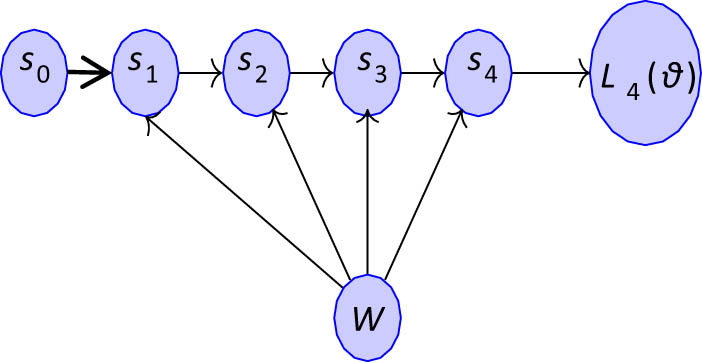
State propagation.

δ S 4 δ w cannot be calculated by simply treating S ₃ as a constant. It can be calculated as shown in the following equation:

(5) δ L t ( θ ) δ S t = δ L t ( θ ) δ S t ∑ k = 1 t δ S t δ S k δ S k δ w .

In such network, L t ( υ ) depends on S _t. S _t depends on S t − 1 and W, S t − 1 in turn, it depends on S t − 2 and so on. This is called backpropagation through time. During backpropagation through time, the magnitude of δ S t δ S k will be very small or very large. So, δ L t δ w will vanish or explode. This problem is known as vanishing or exploding gradients. This can be avoided by truncating backpropagation.

Gated recurrent unit

In traditional RNN, the old information gets morphed by current information at each new timestamp (t). It would be tough to get old information from previous time steps. Some problem occurs during backpropagation. So, there is a need to selectively read, write, and forget information to identify the responsible gradient, which causes the error. Numerous variations like LSTM and gated recurrent unit (GRU) are used to avoid the above-said problem. We have used GRU to deal with vanishing or exploding gradient problems.

In GRU, New input x _t is overloaded with S t − 1 at timestamp t − 1 to compute the new state S t . Here, we returned only necessary information in S t from S t − 1 . We introduced a vector O t − 1 (output gate) which decides what fraction of each element of S t − 1 should be passed to the next state. Learning with another parameter ( W , U , V ) as shown in the following equation is computed as O t − 1 .

(6) O t − 1 = σ ( W 0 S t − 1 + U 0 x t − 1 + b 0 ) .

Parameters W 0 , U 0 , and b 0 are learned along with existing ( W , U , V ) .

S t capture all the information from the previous state and current input x t . However, we want to use only selective information to construct a state S t . This is done by the input gate, as shown in equation (7).

(7) i t = σ ( W i S t − 1 + U i x t + b i ) .

i t ⊙ S t ̌ is used for selective read state information. We combine the previous state S t − 1 and S t ̌ to get a new state.

(8) S t ̌ = σ ( W ( O t ⨀ S t − 1 ) + U x t + b ) ,

(9) S t = ( 1 − i t ) ⨀ S t − 1 + i t ⨀ S t .

Here, forget gate is not used. Both the gates are combined, which depends directly on S t − 1 .

During forward propagation, the gates control the flow of information. They prevent any irrelevant information from being written to the state. Similarly, they control the flow of gradients during backward propagation. During the backward pass, the gradient will get be multiplied by the gate.

Encoder–Decoder

In Enc–Dec architecture, both are neural networks. The decoder takes encoder output as input in every step. We design Enc–Dec architecture by selecting the appropriate encoder, decoder, parameter, and loss function. We used GRU in the encoder as well as the decoder. Further, we used the attention mechanism to make Enc–Dec architecture more expressive.

All information from the encoder is not essential to decode at each timestamp. Only relevant information is fed up to the decoder at a given timestep. The decoder is fed with relevant information from the data by using the following equations:

(10) e jt = f ATT ( S t − 1 − C j ) ,

(11) e jt = V att T tanh ( U att S t − 1 + W att C j ) .

This is useful to capture the importance of jth input from the encoder to get ith the output of the decoder. The softmax function normalizes three weights.

(12) α jt = exp ( e jt ) ∑ J = 1 M exp ( e jt ) .

It shows the probability of getting jth input to produce the tth output. α is learned based on the same parameter used in the Enc–Dec model with the COCOB optimizer.

COCOB optimizer

Most of the optimization algorithms in deep learning and machine learning are based on the parameters like k in k-nearest neighbor and various hyperparameters in deep learning architecture. We are not sure about the computational price and complexity of such an algorithm. So, we thought to use a parameter-free optimization algorithm. In deep learning architecture, optimization is essential. Selection of learning rate for faster convergence is a black art. A small learning rate takes more time to reach an optimal solution whereas a significant learning rate overshoots the optimal solution. Adaptive learning rates adapt to the seal of each coordinate but do not adapt to the distance from the optimal solution. Learning rate is difficult to tune because the distance from the initial learning rate to the optimal solution is unknown and hard to predict. So, it is difficult to achieve a convergence rate O G ∥ x ⁎ x t ∥ t log ( G ∥ x ⁎ − x t ∥ ) t = 1 + 1 T . The only solution is to try different learning rates.

COCOB avoids the use of a learning rate. It started optimization from stochastic optimization which was converted from online optimization where we tried to minimize loss based on knowledge of gradient. This is done by the following algorithm:

for t = 1 to T do

Get x t from the online learning algorithm

Receive stochastic gradient g t such that

E t [ g t ] = ∇ f ( x t )

pass loss l t ( x ) = 〈 g t , x 〉 to the online learning algorithm

end for

return x T ̅ = 1 T ∑ t = 1 T x t

Some famous online algorithms are designed to work in adversarial settings and have a O ( T ) regret bound. They can also be used as stochastic optimization algorithms with O 1 T convergence rate.

Nemirovsky finds a way of getting an optimal learning rate, but it does not work in a stochastic setting [24]. Learning rate defines stepwise approach to reach optimal solution by η t = α T ∥ ∇ F ( x t ) ∥ where α = 1 , 2 , 4 … . 2 n . Streeter proposed a method of getting a learning rate where the learning rate got doubled for every unsuccessful acceleration [25].

COCOB gives a new interpretation to optimization as gambling, compression, and prediction with log loss. The wealth after the T round will be at least H ∑ t = 1 T C t for any random coin flip. A better convergence rate depends on a better betting strategy. COCOB tries to reach an optimal solution as fast as possible. COCOB guarantees second-order bound as follows:

β t = 0 , Wealth o = 1

‘for t = 1 to T do’

play x t = β t Wealth t − 1

Get gradient g t , define l t ( β ) = − log ( 1 − β g t )

Compute Z t = l t ( β t ) = g t 1 − β g t

Set β t + 1 = clip ( β t − Z t 1 + ∑ i = 1 t z i 2 , − 1 2 , 1 2 )

Set Wealth t = Wealth t − 1 − g t x t

end for

Mathew’s correlation coefficients (MCC) and segment of overlap (SOV)

The MCC is given for particular state(s) which belongs to {H,E,C} and {G,H,I,E,B,T,S,L}.

(13) MCC s = p m × i m − u m × o m ( p m + u m ) × ( p m + 0 m ) × ( n m + u m ) × ( n m + 0 m ) ,

where

p m = R mm , i m = ∑ j ≠ m 3 / 8 ∑ k ≠ m 3 / 8 R jk , o m = ∑ j ≠ m 3 / 8 R mj .

The SOV measures the average overlap between the observed and predicted state. The SOV of all states is given by the following equation:

(14) SOV = 1 i m ∑ m ∈ OV S ∑ states ( m ) LOV ( O , P ) + Del ( O , P ) HOV ( O , P ) × Size ( states ) ,

where O and P are observed and predicted structure in the given states, OV S is the number of overlapping states between O and P, LOV ( O , P ) is the actual overlap, HOV ( O , P ) is the length of the common residues for O and P in state m, and i m is a number of residues observed in a given state. Del is the minimum difference between LOV and HOV, LOV, 0.5 × size (O) and 0.5 × size (P). Size (states) is the number of residues in given states.

Proposed methodology

This article presents a model which consists of an RNN, GRU, Enc–Dec, and attention mechanism. Training of this architecture with a modified COCOB optimizer is also presented. The proposed architecture is based on a GRU and a focused attention mechanism. It aims to provide a simple and efficient way to extract information from a source. This means that it needs to handle long sequences. The attention mechanism is used with the Enc–Dec network to handle long sequences. Here, instead of trying to encode a whole sentence, it selects a subset of vectors that can be used to translate the input. This method eliminates the need to store all of the information from the input sequence.

In the context of protein secondary structure prediction using neural networks, padding is often introduced to standardize the length of protein sequences, allowing for efficient batch processing during training. When representing protein sequences and their secondary structures in a format suitable for neural network training, encoding is essential. Amino acids are typically encoded using a numerical or one-hot encoding scheme. In a one-hot encoding, each amino acid is represented as a binary vector with all zeros except for the position corresponding to the index of the amino acid, which is set to 1. The padding is also represented using the same encoding scheme. However, a special token or vector is assigned to represent the padding. This token could be an additional binary vector of the same length as the amino acid vectors, with all zeros except for a special index set to 1.

All sequences, including the padded ones, are standardized to a fixed length of 700 residues. The amino acid vectors for the actual amino acids and the padding vector are concatenated to create the final input sequence for the neural network. Similarly, the secondary structure information is encoded for each residue in the sequence. Commonly, secondary structures like helix, sheet, and coil are represented using numerical values or one-hot encoding. For example, a three-class classification could use [1, 0, 0] for helix, [0, 1, 0] for sheet, and [0, 0, 1] for coil. The predicted output for the padding residues will also have a corresponding representation. The output layer of the neural network, which performs the classification, will generate a vector indicating the predicted secondary structure for each residue, including the padding residues.

Encoder

The GRU encoder has an input amino acid sequence like S, K, etc. Encoder states are indicated by c ₁, c ₂, c ₃ … c _n−1. The encoder yields a solitary result vector c passed as an input to the decoder. The input of the model is an amino acid sequence which is stored in vector A. A = ( A 1 … . . A T A ) , A ∈ R K A and output is given by B = ( B 1 … . . B T B ) , B ∈ R K B where the size of input and output is given by K A and K B and the length of input and output is given by T A and T B .

Decoder

The decoder has additional solitary layered GRU. Decoder states are addressed by s ₁, s ₂, s ₃, s _n−1. There are eight secondary structures named G, H, I, E, B, T, S, and L in the model as output. The issue with this design is that it uses a single vector c to represent the whole sequence. The hidden state S i of the decoder from the encoder is calculated by S i = ( 1 − Z i ) ⊙ Z i ⨀ S i ̌ .

Where

(15) S i = tanh ( WE B i − 1 + ̌ U [ r i ⨀ S i − 1 ] + C c i ,

(16) Z i = σ ( W z E B i − 1 + U z S i − 1 + C z C i ) ,

(17) r i = σ ( W r E B i − 1 + U r S i − 1 + C r C i ) ,

where E is the embedding matrix of the target protein structure. W 1 , W z , W r ϵ R n × m , U 1 , U z , U r ϵ R n × n , C 1 , C z , C r ϵ R n × 2 n are weights. The initial hidden states S 0 = tanh ( W s h 1 ← ) , where W s ∈ R n × n . Context vectors C i = ∑ j = 1 T x α ij h j where h j is the jth annotation in the input sequence.

Attention

We used attention mechanism which allows the model to focus on different parts of the input sequence when generating each element of the output sequence. In sequence-to-sequence tasks, the goal is to map an input sequence to an output sequence. The Bahdanau Attention Mechanism introduces the concept of “context vectors.” These are dynamically calculated weighted sums of the encoder’s hidden states, and they provide the decoder with relevant information for generating each element of the output sequence [26]. Instead of using a fixed context vector for the entire decoding process, Bahdanau attention computes the alignment scores for each pair of encoder and decoder hidden states. These scores represent how well the current decoder state aligns with each encoder state.

The alignment scores are transformed into attention weights using the softmax function. These weights determine the importance of each encoder state in calculating the context vector. The context vector is then calculated as the weighted sum of the encoder hidden states, where the weights are given by the attention weights. This dynamic calculation allows the model to selectively focus on different parts of the input sequence during the generation of each output element. The context vector is concatenated with the input to the decoder, providing additional information about the relevant parts of the input sequence for generating the next output element. During training, the attention mechanism is trained alongside the rest of the model parameters. The attention weights are learned through backpropagation, allowing the model to learn which parts of the input are important at different decoding steps.

The Bahdanau attention mechanism allows the model to handle cases where different parts of the input sequence contribute differently to different parts of the output sequence. This is especially useful for tasks where the alignment between input and output sequences is not strictly monotonic. The attention mechanism provides flexibility by allowing the model to attend to different parts of the input sequence at each decoding step.

The attention system combined with the GRU enables it to focus on specific pieces in the input sequence to predict the state. This makes it an essential part of the network’s algorithm for prediction tasks. The attention model is composed of a single-layer GRU encoder and a decoder. Its inputs consist of the encoder’s result h _i and the decoder’s state. The output of the attention is referred to as context vectors c _i.

Our attention model has a single-layer GRU encoder, again with n-time steps. We denote the encoder’s input vectors by S, K, etc. and the result vectors by h ₁, h ₂, h ₃, h ₄, h _n. The attention mechanism is situated between the encoder and the decoder; its input is made out of the encoder’s result vectors h ₁, h ₂, h ₃, h ₄… h _n and the states of the decoder are s ₀, s ₀, s ₂, s ₃ … s _n−1. The attention’s result is a sequence of context vectors denoted by c ₁, c ₂, c ₃, c ₄ … c _n. The context vectors help the decoder to focus on certain parts of the sequence. It consists of an ith vector of its input. This allows it to identify the essential parts of the input. Figure 3 depicts the proposed architecture.

Figure 3

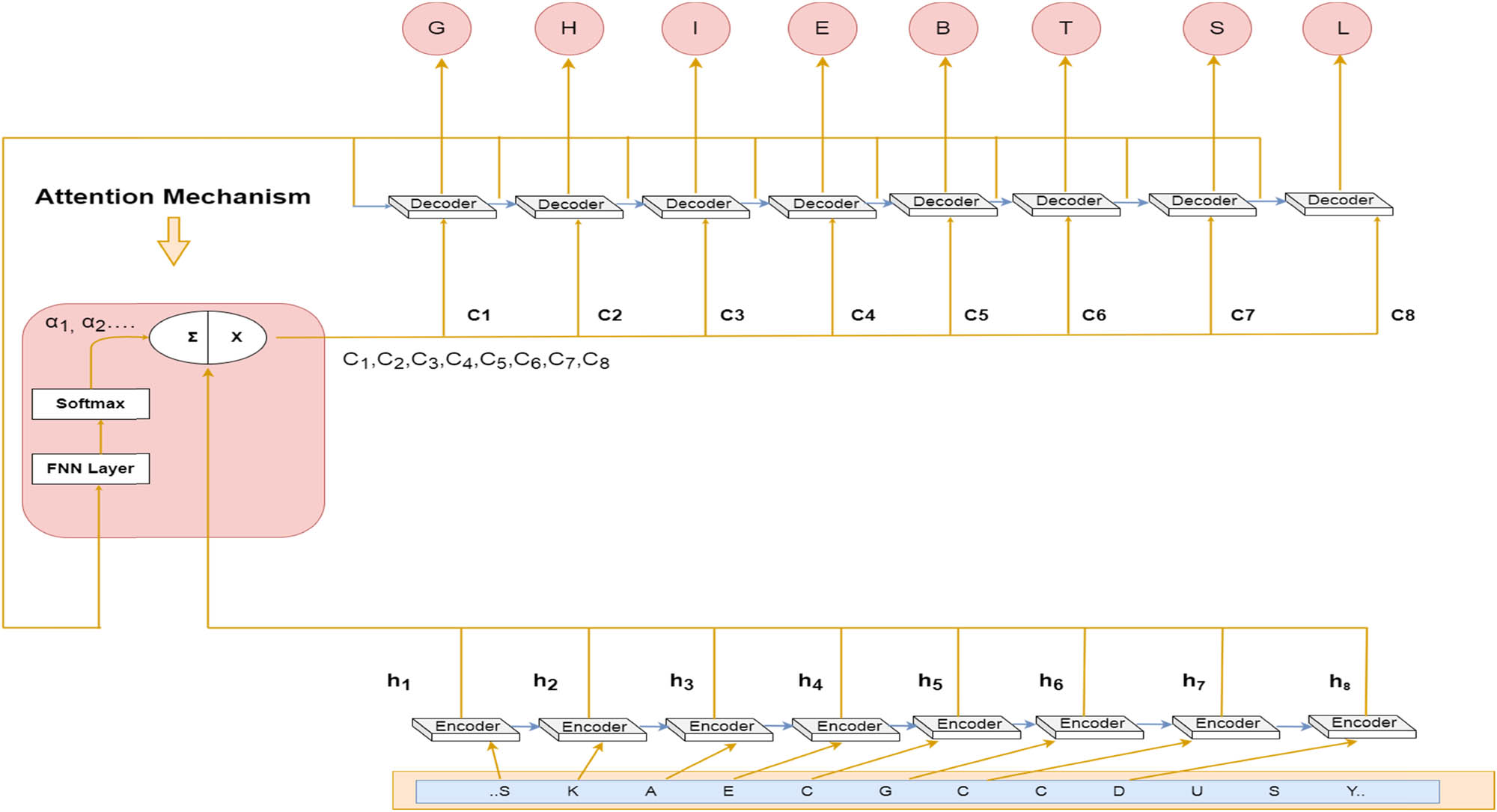
Architecture of the proposed algorithm.

Data preparation and experimental setup

Data preparation

Our algorithms were used on two open datasets, CB513 and CullPDB. CullPDB is a non-homologous dataset that has an identity of less than 30%. It consists of 6,128 protein amino residues labeled with Q ₈ secondary labels. It is randomly divided into 5,600 training, 248 validation, and 280 testing sets. CB513 contains 513 proteins which are filtered CullPDB. CB513 is divided into 410 training samples and 104 validation sets [27].

PSI_BLAST assigns each amino acid to one of the eight secondary structures which are H (α-helix), G (3-helix or 310-helix), I (5-helix or P-helix), β (residue in isolated beta-bridge), E (extended sheet), T (hydrogen bond turn), S (bend), and “-” (any other structure). These eight secondary structures are reduced to three-state helix (H), sheet (E), and coil (C). The critical assessment of structure prediction reduction method assigns (H, G, I to H), (E, B to E), and all other states to C.

Eight neurons encode secondary classes at the output layer with the following binary representation:

G = [1 0 0 0 0 0 0 0]

H = [0 1 0 0 0 0 0 0]

I = [0 0 1 0 0 0 0 0]

E = [0 0 0 1 0 0 0 0]

B = [0 0 0 0 1 0 0 0]

T = [0 0 0 0 0 1 0 0]

S = [0 0 0 0 0 0 1 0]

L = [0 0 0 0 0 0 0 1].

H = [1 0 0],

E = [0 1 0],

C = [0 0 1].

Experimental set-up

RNN and GRU in this article have the size of hidden layer 300 and a fully connected output layer consisting of 3 and 8 neurons for Q 3 and Q 8 classification, respectively. Python Spyder, v5.1.1 tool is used for implementation with Keras 2.4.0 for neural network packages where TensorFlow v2.6.0 is running on the top. Our networks consist of a dense layer for dot multiplication and bias function, an activation function to initiate the learning tasks and a dropout layer to avoid overfitting.

Parameter initialization

We have started with the random orthogonal matrix weights. We then sampled each element from the random distribution of the mean 0 and variance 0.001 2 . The dropout value of 0.6 was set to minimize the error. The COCOB optimizer typically learns repeated features by continuously updating the hyperparameter. The batch size 128, the epoch value 200, and the loss/error over the training set are fixed and executed.

Training procedure

We trained our entire deep neural network with a COCOB optimizer. As per our previous work, the COCOB optimizer worked better than other optimizers. The training data were passed in 128 sequences to avoid computational inefficiency. Dropout regularization is used to avoid overfitting in this model. Here, we are presenting the training on the Enc–Dec model with an attention mechanism. The network is given amino acid features to get the protein chain’s residue as an output. The attention model predicts the Q ₈ state from the input sequence generated by the encoder.

The attention weights are learned through a softmax function and an external network. They represent the importance of h _j in deciding the next hidden state. A significant attention weight can cause the GRU to focus only on the input x _j. The f _c network is trained to handle the GRU’s prediction error terms by backpropagation. This process is carried out through the decoder and the f _c attention network.

This mechanism aims to allow the decoder to pay attention to the various parts of the input sequence. This allows the encoder to avoid encoding all of the information in the sequence into a single vector. The training algorithm is shown as follows:

Initialization:

Input data:

β t = 0 , Wealth o = 1

x = { x 1 , x 2 … . x N } protein sequence of length N

S _ t = timestamp at t

Encoder:

Forward propagation:

for t = 1 to N do

O t − 1 = σ ( W 0 S t − 1 + U 0 x t − 1 + b 0 )

i t = σ ( W i S t − 1 + U i x t + b i )

S t ̌ = σ ( W ( O t ⨀ S t − 1 ) + U x t + b )

S t = ( 1 − i t ) ⨀ S t − 1 + i t ⨀ S t

end for

Backward propagation:

for all t ∈ ( 1 , 2 , … N ) do

x t = β t S t − 1

l t ( β ) = − log ( 1 − β g t )

Z t = l t ( β t ) = g t 1 − β g t

β t + 1 = clip β t − Z t 1 + ∑ i = 1 t z i 2 , − 1 2 , 1 2

S t = S t − 1 − g t x t

end for

Attention:

for t = 1 to N do

for j = 0 to N do

e jt = f ATT ( S t − 1 − C j )

e jt = V att T tanh ( U att S t − 1 + W att C j )

α jt = exp ( e jt ) ∑ J = 1 M exp ( e jt )

end for

Decoder:

for i = 1 to N do

C i = ∑ j = 1 t α ij h j

end for

Forward Propagation:

for t = 1 to N do

O t − 1 = σ ( W 0 S t − 1 + U 0 C t − 1 + b 0 )

i t = σ ( W i S t − 1 + U i C t + b i )

S t ̌ = σ ( W ( O t ⨀ S t − 1 ) + U C t + b )

S t = ( 1 − i t ) ⨀ S t − 1 + i t ⨀ S t

end for

Backward propagation:

for all t ∈ ( 1 , 2 , … N ) do

C t = β t S t − 1

l t ( β ) = − log ( 1 − β g t )

Z t = l t ( β t ) = g t 1 − β g t

β t + 1 = clip β t − Z t 1 + ∑ i = 1 t z i 2 , − 1 2 , 1 2

S t = S t − 1 − g t C t

end for

Results

Our model evaluated the accuracy of protein secondary structure by Q ₃, Q ₈, Mathew correlation coefficients, and SOV. Q ₃, Q ₈, and MCC predict individual amino acids. Accuracy based on single residues does not guarantee the overall accuracy of protein secondary structure. Because some secondary structure states depend on adjacent amino acids. We are using SOV scores to guarantee the accuracy of protein secondary structure prediction.

Matrix with a size 3 × 3 and 8 × 8 is defined to measure accuracy. R _mn represented the number of residues observed in state m and predicted as the state n. The parameters m and n belong to {H,E,C} and {G,H,I,E,B,T,S,L} for Q ₃ and Q ₈ accuracy respectively.

(18) Q 3 = 1 i ∑ m = 1 3 R mm ,

(19) Q 8 = 1 i ∑ m = 1 8 R mm .

i is the total number of residues.

The accuracy of the individual secondary structures is calculated as Q i = 1 i m R mn where i m is the total number of residues in state m.

Our algorithms are tested on CullPDB and CB513 datasets. Q ₃ and Q ₈ accuracies observed for the CullPDB and CB513 dataset by using RNN, GRU, Enc–Dec, and Enc–Dec with attention mechanism are shown in Figure 3. We achieved a Q ₃ accuracy on the CullPDB dataset of 59.23, 62.13, 69.87, and 70.69% for RNN, GRU, Enc–Dec, and Enc–Dec with attention mechanism respectively. We achieved a Q ₃ accuracy on the CB513 dataset of 69.17, 73.18, 77.86, and 79.38% for RNN, GRU, Enc–Dec, and Enc–Dec with an attention mechanism. We achieved a Q ₈ accuracy on CullPDB dataset of 60.34, 63.92, 76.28, and 78.93% for RNN, GRU, Enc–Dec, and Enc–Dec with attention mechanism, respectively. We achieved a Q ₈ accuracy on CB513 dataset of 68.73, 72.80, 75.89, and 77.13% for RNN, GRU, Enc–Dec, and Enc–Dec with attention mechanism, respectively. We have found that Enc–Dec with attention mechanism model gives better results on CullPDB and CB513 datasets which is shown in Figure 4.

Figure 4

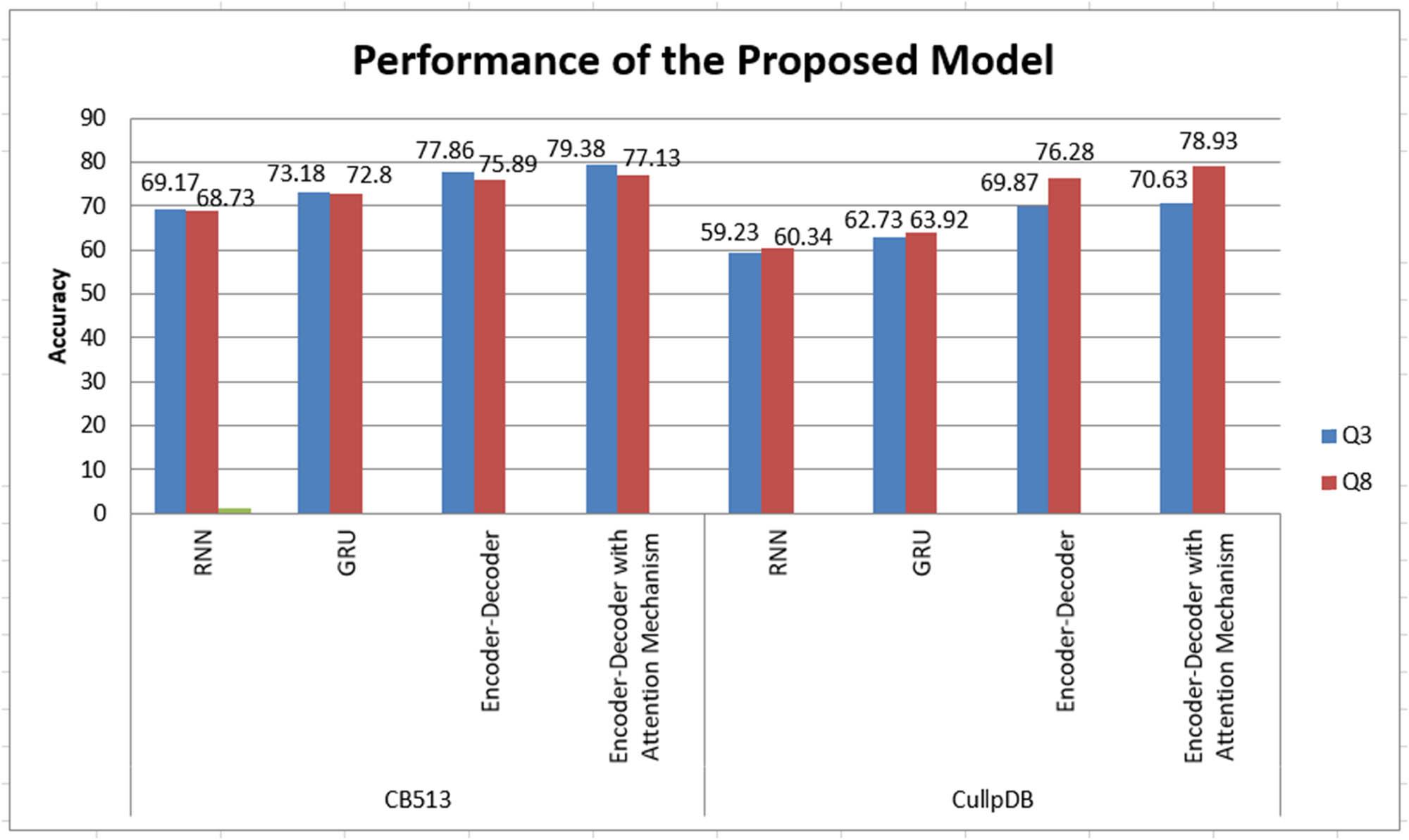
Performance of the proposed model.

The corresponding Q H (Helix Accuracy), Q E (Sheet Accuracy), Q C (Coil Accuracy) obtained for the CullPDB and CB513 datasets by using our models are shown in Table 1. We achieved corresponding Q _H accuracy on the CullPDB dataset of 61.10, 61.28, 74.42, and 73.23% for RNN, GRU, Enc–Dec, and Enc–Dec with attention mechanism respectively. We achieved corresponding Q _E accuracy on the CullPDB dataset of 60.23, 64.23, 75.31, and 74.91% for RNN, GRU, Enc–Dec, and Enc–Dec with attention mechanism respectively. We achieved corresponding Q _C accuracy on the CullPDB dataset of 59.6, 62.10, 70.23, and 76.82% for RNN, GRU, Enc–Dec, and Enc–Dec with attention mechanism respectively. We achieved 70.3, 69.24, and 71.30% Q _H, Q _E, and Q _C accuracy, respectively on CB513 dataset for RNN. We achieved 72.10, 73.20, and 70.23% Q _H, Q _E, and Q _C accuracy, respectively, on the CB513 dataset for GRU. We achieved 78.13, 71.37, and 73.24% Q _H, Q _E, and Q _C accuracy, respectively, on CB513 dataset for Enc–Dec. We achieved 80.23, 79.14, and 78.92% Q _H, Q _E, and Q _C accuracy, respectively, on the CB513 dataset for Enc–Dec with an attention mechanism.

Table 1

Performance of the proposed method

Dataset	Architecture	SOV (%)	SOV_H (%)	SOV_E (%)	SOV_C (%)	C _H	C _E	C _C
CB513	RNN	79.83	78.1	76.23	77.03	0.81	0.84	0.97
	GRU	84.34	81.03	83.10	84.01	0.80	0.80	0.81
	Encoder–decoder	88.10	87.07	86.71	88.09	0.92	0.97	0.91
	Encoder–decoder with attention mechanism	91.3	90.03	92.43	90.10	0.94	0.90	0.89
CullPDB	RNN	76.26	74.11	77.23	78.93	0.83	0.87	0.71
	GRU	77.13	75.21	79.29	80.13	0.85	0.89	0.78
	Encoder–decoder	78.92	80.13	77.18	79.33	0.81	0.90	0.76
	Encoder–decoder with attention mechanism	80.29	82.13	81.28	78.13	0.88	0.92	0.79

SOV scores and MCC measurements observed on CullPDB and CB513 for our models are shown in Table 1. We achieved 79.83, 84.34, 88.10, and 91.3% SOV scores for RNN, GRU, Enc–Dec, and Enc–Dec with attention mechanism on CB513, respectively. We achieved 76.26, 77.13, 78.92, and 80.29% SOV scores for RNN, GRU, Enc–Dec, and Enc–Dec with attention mechanism on CullPDB, respectively. We achieved 0.81, 0.80, 0.92, and 0.94 corresponding MCCs for helix (C _H), respectively, on the CB513 dataset for RNN, GRU, Enc–Dec, and Enc–Dec with attention mechanism, respectively. We achieved 0.84, 0.80, 0.97, and 0.90 corresponding MCCs for sheet (C _E), respectively, on the CB513 dataset for RNN, GRU, Enc–Dec, and Enc–Dec with attention mechanism, respectively. We achieved 0.97, 0.81, 0.91, and 0.89 corresponding MCCs for sheet (C _C) accuracy respectively on the CB513 dataset for RNN, GRU, Enc–Dec, and Enc–Dec with attention mechanism, respectively. We achieved 0.83, 0.85, 0.81, and 0.88 corresponding C _H accuracy, respectively, on the CullPDB dataset for RNN, GRU, Enc–Dec, and Enc–Dec with attention mechanism, respectively. We achieved 0.87, 0.89, 0.90, and 0.92 corresponding C _E accuracy, respectively, on the CullPDB dataset for RNN, GRU, Enc–Dec, and Enc–Dec with attention mechanism, respectively. We achieved 0.71, 0.78, 0.76, and 0.79 corresponding C _C accuracy, respectively, on the CullPDB dataset for RNN, GRU, Enc–Dec, and Enc–Dec with attention mechanism, respectively, which is shown in Table 1.

Discussion

We have compared all the evaluating parameters of our model with a few of the existing models. It is observed that our model is performing better than the existing models. We have compared our model with BRNN [28], CNF [29], GSN [4], LSTM [3], SSREDN [5], and 1D-Convnet and 1D-Convnet with BLSTM [30]. Q ₈ comparison on CB513 is shown in Table 2. Our model achieved 77.13% Q ₈ accuracy and observed significant improvement in the performance as compared to another model in the literature.

Table 2

Q ₈ accuracy comparison of the proposed method with literature methods on CB513

Model	Q ₈ accuracy (%) on CB513
BRNN	51.1
CNF	64.9
GSN	66.4
LSTM	67.4
SSREDN	68.2
1D-ConvNet	73.3
1D-ConvNet with BLSTM	74.45
Encoder–decoder	75.89
Encoder–decoder with attention	77.13

We have compared our model with SSpro [31], RaptorX-SS8 [32], GSN, SSREDN, 1D-Convnet and 1D-Convnet with BLSTM. Q ₈ comparison on CullPDB dataset is shown in Table 3. Our model achieved 78.93% Q ₃ accuracy and observed significant improvement in the performance as compared to other models in the literature.

Table 3

Q ₈ accuracy comparison of proposed method with literature methods on CullPDB

Model	Q ₈ accuracy (%) on CullPDB
SSpro	66.6
RaptorX-SS8	69.7
GSN	72.1
SSREDN	73.1
1D-Convnet	64.48
1D-Convnet with BLSTM	75.04
Encoder–decoder	76.28
Encoder–decoder with attention	78.93

We have compared our model with SSpro, RaptorX-SS8, PSIPRD, and 1D-Convnet with BLSTM for Q ₃ accuracy. Q ₃ comparison on the CB513 dataset is shown in Table 4. Our model achieved 78.93% Q ₃ accuracy and observed significant improvement in the performance as compared to another model in the literature.

Table 4

Q ₃ accuracy comparison of proposed method with literature methods on CB513

Model	Q ₃ accuracy (%) on CB513
SSpro	78.5
RaptorX-SS8	78.3
PSIPRD	79.2
1D-Convnet with BLSTM	66.4
Encoder–decoder with attention	79.38

The Q ₈ accuracy measures the overall accuracy of predicting the eight different states of protein secondary structure. If the model is good at distinguishing between the various fine-grained states (Alpha Helix, 3–10 Helix, Pi Helix, Beta Strand, Beta Bridge, Turn, Coil, Bend), it may achieve high accuracy on Q ₈. However, Q ₃ accuracy measures a more coarse-grained classification into three states (Helix, Strand, Coil). Achieving high Q ₃ accuracy requires the model not only to differentiate between fine-grained states but also to correctly group them into the broader categories.

The architecture of the Enc–Dec model plays a crucial role. If the model is more focused on capturing the fine-grained details of the input sequence, it might perform well on Q ₈ but struggle to generalize to the rough Q ₃ classification. The encoding process in the Enc–Dec model might emphasize capturing the detailed features of the input sequence, making it effective for Q ₈ but less suited for the simpler Q ₃ classification. The model might overfit to specific features related to the fine-grained states, making it less robust in grouping them into broader categories. This overfitting could lead to high accuracy on Q ₈ but lower accuracy on Q ₃.

Figures 5 and 6 compare the SOV scores and the MCC measurements for CB513 with SPIDER2, JPred4, RptoX, SSPRO5, and observed a significant improvement in the performance.

Figure 5

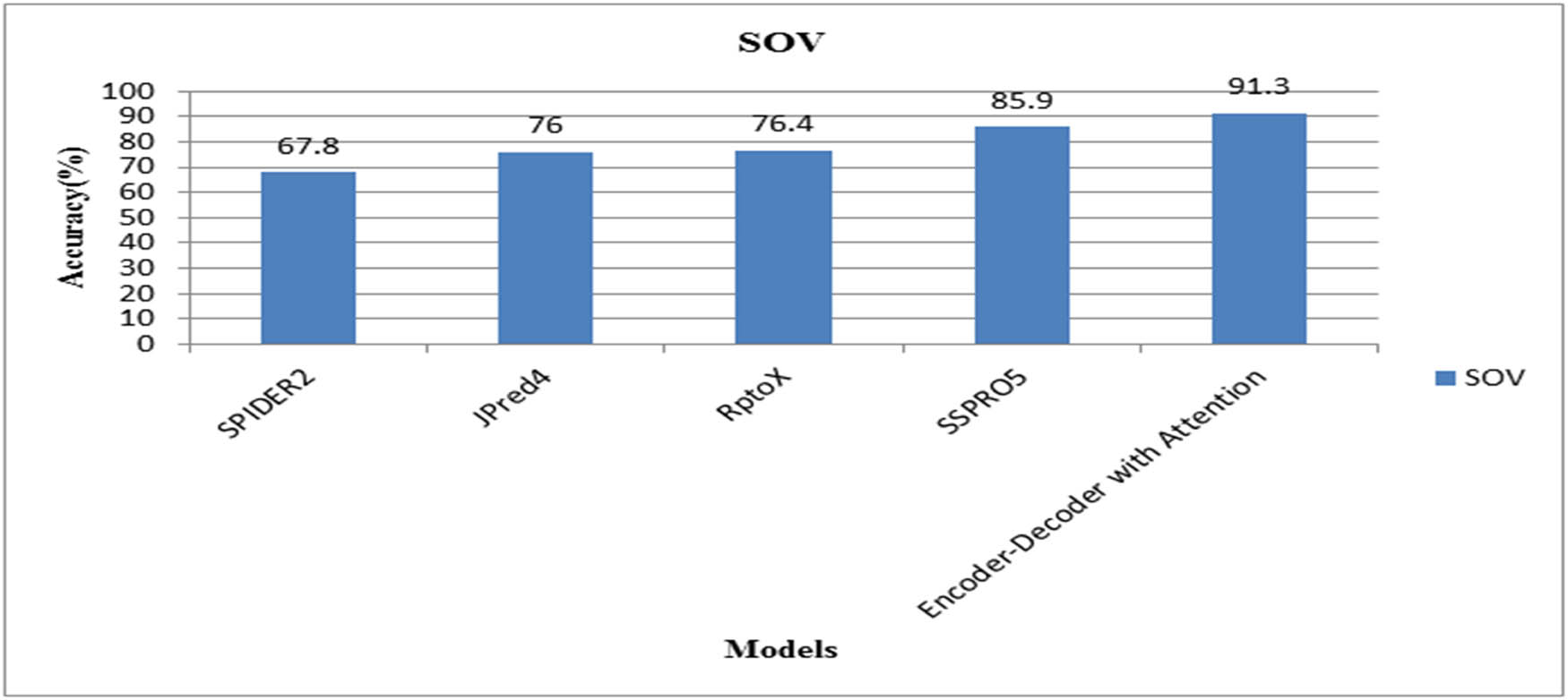
Comparison of SOV with literature methods.

Figure 6

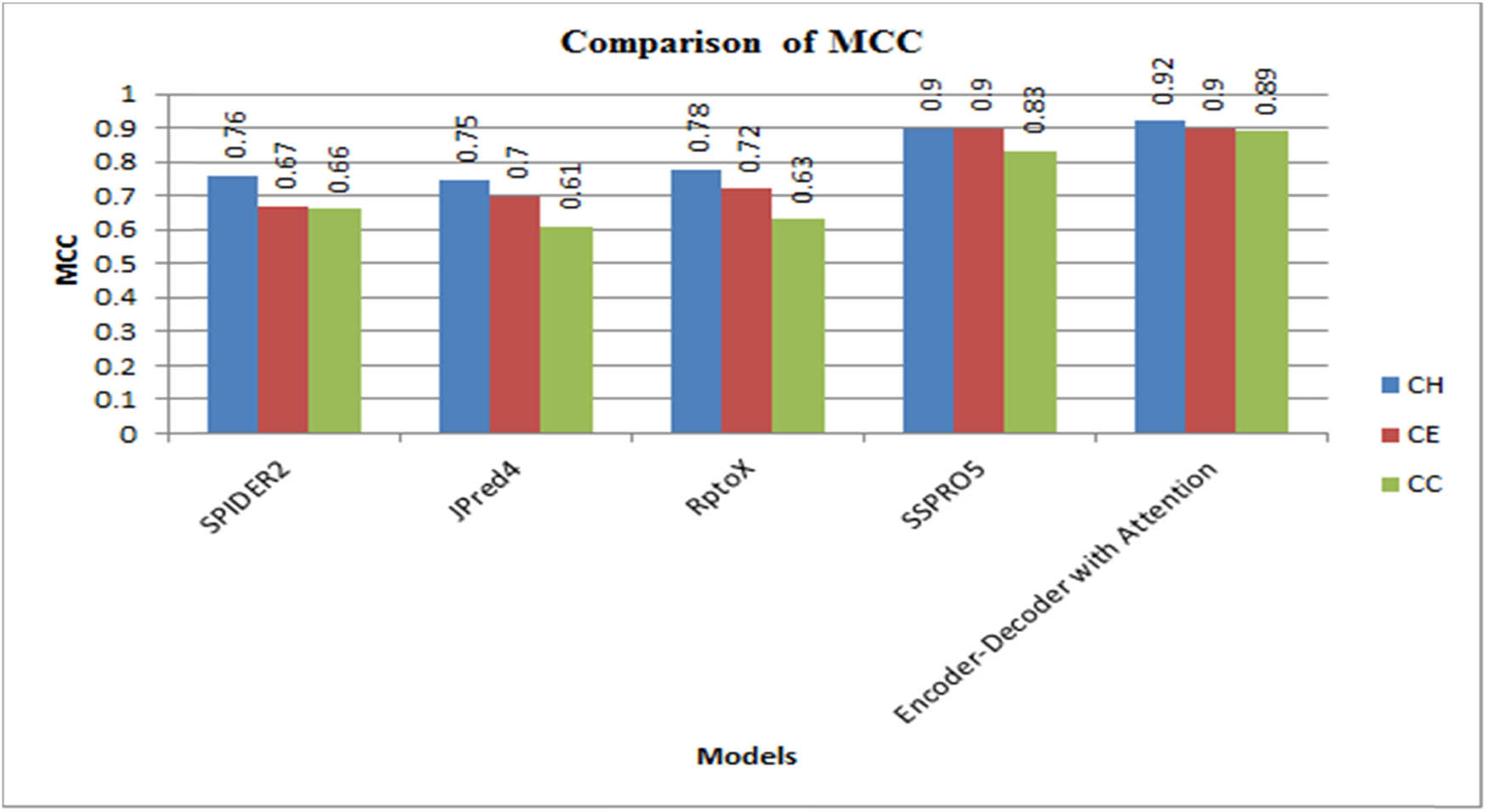
Comparison of MCC with literature methods.

Conclusion and future work

In this article, we have proposed the Enc–Dec model with an attention mechanism to predict the protein structure from amino acid residues. We have started our experimentation with RNN on CB513 and CullPDB open datasets, in which we faced the problem of vanishing gradient. GRU model is used to overcome the vanishing gradient problem. The attention mechanism in our model is used to select prominent features from amino acid residues which helps to increase the performance of our model. We used a modified COCOB optimizer for hypertuning of the hyperparameter. We found significant improvement in Q ₃ accuracy, Q ₈ accuracy, SOV, and MCC using our models. Further, we can improve our model’s Q ₃ accuracy on the CullPDB dataset. As tuning of hyperparameter is the biggest challenge in deep learning, we can further improve the learning ability of our model based on momentum or learning rate.

Acknowledgements

We appreciate the support from the Department of Computer Science and Engineering, Shri Ramdeobaba College of Engineering and Management, Nagpur, for allowing us to experiment on the Nvidia DGX station and the School of Computer Science and Engineering, Vellore Institute of Technology, Vellore.

Funding information: Authors state no funding involved.
Conflict of interest: Authors state no conflict of interest.
Data availability statement: The datasets generated during and/or analysed during the current study are available from the corresponding author on reasonable request.

References

[1] Johnson DK, Karanicolas J. Ultra-high-throughput structure-based virtual screening for small-molecule inhibitors of protein–protein interactions. J Chem Inf Modeling. 2016;56(2):399–411. 10.1021/acs.jcim.5b00572.Search in Google Scholar PubMed PubMed Central

[2] Wood MJ, Hirst JD. Protein secondary structure prediction with dihedral angles. PROTEINS: structure, function, and bioinformatics. Proteins: Struct Funct Bioinf. 2005;59(3):476–81.10.1002/prot.20435Search in Google Scholar PubMed

[3] Sønderby SK, Winther O. Protein secondary structure prediction with long short term memory networks; arxiv.org/abs/1412.7828. 2014.Search in Google Scholar

[4] Zhou J, Troyanskaya OG. Deep Supervised and Convolutional generative stochastic network for protein secondary structure prediction, 31st international conference on machine learning. ICML. 2014;2:1121–9.Search in Google Scholar

[5] Wang Y, Mao H, Yi Z. Protein secondary structure prediction by using deep learning method. Knowl Based Syst. 2017;118:115–23. 10.1016/j.knosys.2016.11.015.Search in Google Scholar

[6] Arian R, Hariri A, Mehridehnavi A, Fassihi A, Ghasemi F. Protein kinase inhibitors’ classification using K-nearest neighbor algorithm. Comput Biol Chem. 2020;86(2019):107269. 10.1016/j.compbiolchem.2020.107269.Search in Google Scholar PubMed

[7] Kim H, Park H. Protein secondary structure prediction based on an improved support vector machines approach. Protein Eng. 2003;16(8):553–60. 10.1093/protein/gzg072.Search in Google Scholar PubMed

[8] Gromiha M, Suwa M. Discrimination of outer membrane proteins using machine learning algorithms. Proteins: Struct Funct Bioinf. 2006;63:1031–7.10.1002/prot.20929Search in Google Scholar PubMed

[9] Lasfar M, Bouden H. A method of data mining using Hidden Markov Models (HMMs) for protein secondary structure prediction. Proc Comput Sci. 2018;127:42–51. 10.1016/j.procs.2018.01.096.Search in Google Scholar

[10] Shu JJ, Yong KY. Fourier-based classification of protein secondary structures. Biochem Biophys Res Commun. 2017;485(4):731–5. 10.1016/j.bbrc.2017.02.117.Search in Google Scholar PubMed

[11] Kathuria C, Mehrotra D, Misra NK. Predicting the protein structure using random forest approach. Proc Comput Sci. 2018;132:1654–62. 10.1016/j.procs.2018.05.134.Search in Google Scholar

[12] Bingru Y, Wei H, Zhun Z, Huabin Q. KAAPRO: An approach of protein secondary structure prediction based on KDD* in the compound pyramid prediction model. Expert Syst Appl. 2009;36(5):9000–6. 10.1016/j.eswa.2008.12.029.Search in Google Scholar

[13] Spencer M, Eickholt J, Cheng J. A deep learning network approach to. IEEE/ACM Trans Comput Biol Bioinf/IEEE, ACM. 2015;12(1):103–12. 10.1109/TCBB.2014.2343960.Search in Google Scholar PubMed PubMed Central

[14] Ibrahim AA, Yasseen IS. Using neural networks to predict secondary structure for protein folding. J Comput Commun. 2017;5(1):1–8. 10.4236/jcc.2017.51001.Search in Google Scholar

[15] Zhou J, Troyanskaya OG. Deep Supervised and Convolutional generative stochastic network for protein secondary structure prediction,” 31st international conference on machine learning. ICML. 2014;2:1121–9.Search in Google Scholar

[16] Khalatbari L, Kangavari MR, Hosseini S, Yin H, Cheung NM. MCP: a multi-component learning machine to predict protein secondary structure. Comput Biol Med. 2019;110:144–55. 10.1016/j.compbiomed.2019.04.040.Search in Google Scholar PubMed

[17] Wang S, Peng J, Ma J, Xu J. Protein secondary structure prediction using deep convolutional neural fields. Sci Rep. 2016;6:1–11. 10.1038/srep18962.Search in Google Scholar PubMed PubMed Central

[18] Zhang B, Li J, Lü Q. Prediction of 8-state protein secondary structures by a novel deep learning architecture. BMC Bioinf. 2018;19(1):1–13. 10.1186/s12859-018-2280-5.Search in Google Scholar PubMed PubMed Central

[19] Xie S, Li Z, Hu H. Protein secondary structure prediction based on the fuzzy support vector machine with the hyperplane optimization. Gene. 2018;642:74–83. 10.1016/j.gene.2017.11.005.Search in Google Scholar PubMed

[20] Babaei S, Geranmayeh A, Seyyedsalehi SA. Protein secondary structure prediction using modular reciprocal bidirectional recurrent neural networks. Comput Methods Prog Biomedicine. 2010;100(3):237–47. 10.1016/j.cmpb.2010.04.005.Search in Google Scholar PubMed

[21] Li Z, Yu Y. Protein secondary structure prediction using cascaded convolutional and recurrent neural networks. IJCAI Int Jt Conf Artif Intell. 2016;2016:2560–7.Search in Google Scholar

[22] Liu Z, Li Z, Li L, Yang H. Complex background classification network: a deep learning method for urban images classification. Comput Electr Eng. 2020;87:106771. 10.1016/j.compeleceng.2020.106771.Search in Google Scholar

[23] Guo Y, Wang B, Li W, Yang B. Protein secondary structure prediction improved by recurrent neural networks integrated with two-dimensional convolutional neural networks. J Bioinf Comput Biol. 2018;16(5):1850021. 10.1142/S021972001850021X.Search in Google Scholar PubMed

[24] Nazin AV, Nemirovsky AS, Tsybakov AB, Juditsky AB. Algorithms of robust stochastic optimization based on mirror descent method. Autom Remote Control. 2019;80(9):1607–27. 10.1134/S0005117919090042.Search in Google Scholar

[25] Streeter M, McMahan HB. No-regret algorithms for unconstrained online convex optimization. Adv Neural Inf Process Syst. 2012;3:2402–10.Search in Google Scholar

[26] Vaswani A, Shazeer N, Parmar N, Uszkoreit J, Jones L, Gomez AN, et al. Attention is all you need. Adv Neural Inf Process Syst. 2017;30:5999–6009.Search in Google Scholar

[27] Sonsare P, Gunavathi C. Optimization based long short term memory network for protein structure prediction. U Porto J Eng. 2022;8(2):108–20. 10.24840/2183-6493_008.002_0009Search in Google Scholar

[28] Pollastri G, Przybylski D, Rost B, Baldi P. Improving the prediction of protein secondary structure in three and eight classes using recurrent neural networks and profiles. Proteins: Structure, Function, and Bioinformatics. 2002;47(2):228–35.10.1002/prot.10082Search in Google Scholar PubMed

[29] Wang J, Zhiyong, Zhao, Feng, Peng, et al. Protein 8-class secondary structure prediction using conditional neural fields. Proteomics. 2011;3786–92.10.1002/pmic.201100196Search in Google Scholar PubMed PubMed Central

[30] Sonsare PM, Gunavathi C. Cascading 1D-convnet bidirectional long short term memory network with modified COCOB optimizer: a novel approach for protein secondary structure prediction. Chaos, Solitons Fractals. 2021;153:111446. 10.1016/j.chaos.2021.111446.Search in Google Scholar

[31] Magnan P, Baldi CN. SSpro/ACCpro 5: almost perfect prediction of protein secondary structure and relative solvent accessibility using profiles, machine learning and structural similarity. Bioinformatics. 2014;30:2592–7.10.1093/bioinformatics/btu352Search in Google Scholar PubMed PubMed Central

[32] Peng J, Xu J. RaptorX: exploiting structure information for protein alignment by statistical inference. Proteins. 2011;79:161–71.10.1002/prot.23175Search in Google Scholar PubMed PubMed Central

Received: 2023-10-18

Revised: 2024-02-07

Accepted: 2024-02-09

Published Online: 2024-03-13

This work is licensed under the Creative Commons Attribution 4.0 International License.

Articles in the same Issue

https://doi.org/10.1515/bmc-2022-0043

Keywords for this article

bioinformatics; machine learning; deep learning; protein secondary structure prediction

Creative Commons

BY 4.0