US household deleveraging following the Great Recession – a model-based estimate of equilibrium debt
-
Bruno Albuquerque
 ,
Ursel Baumann
,
Ursel Baumann

Abstract
The balance sheet adjustment in the household sector was a prominent feature of the Great Recession that is widely believed to have held back the cyclical recovery of the US economy. A key question for the US outlook is therefore whether household deleveraging has ended or whether further adjustment is needed. The novelty of this paper is to estimate a time-varying equilibrium household debt-to-income ratio determined by economic fundamentals to examine this question. The paper uses state-level data for household debt from the FRBNY Consumer Credit Panel over the period 1999Q1–2012Q4 and employs the Pooled Mean Group (PMG) estimator developed by Pesaran, Shin, and Smith (1999), adjusted for cross-section dependence. The results support the view that, despite significant progress in household balance sheet repair, household deleveraging still had some way to go as of 2012Q4, as the actual debt-to-income-ratio continued to exceed its estimated equilibrium. The baseline conclusions are rather robust to a set of alternative specifications. Going forward, our model suggests that part of this debt gap could, however, be closed by improving economic conditions rather than only by further declines in actual debt. Nevertheless, the normalisation of the monetary policy stance may imply challenges for the deleveraging process by reducing the level of sustainable household debt.
Appendix A
A Deriving the Common Correlated Effects Pooled Mean Group (CCEPMG) equation
We estimate a dynamic panel error correction model based on quarterly data for 50 US states (plus the District of Columbia) over the period 1999Q1–2012Q4, with subindices t=1, 2,..., T (T=56) for quarters and i=1, 2,..., N (N=51) for states. Following Pesaran, Shin, and Smith (1999), we assume an autoregressive distributed lag (ARDL) (1,1,1,...,1) dynamic panel specification of the form:
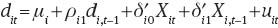
where
If the variables are I(1) and cointegrated, then the error term is I(0) for all i.
Using dit=di, t–1+Δdit, (1) can be written as:

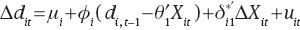
Furthermore, since Xi, t–1=Xit–ΔXit, we can write the above equation as:

To highlight the long-run relationship, we can write (3) in error-correction form:

where
To estimate the parameters of the model, we apply the Pooled Mean Group (PMG) estimator as described in Pesaran, Shin, and Smith (1999). Under the PMG estimator assumption of long-run homogeneity, the long-run coefficients are assumed to be the same across states, i.e., θi1=θ1. By contrast, the short-run coefficients and the group-specific error correction coefficients (the speed of adjustment) are allowed to differ across states, so that δij=δij, and ϕi=ϕi. In this case, the reported coefficient values are given by the means of the respective estimates for individual states. The PMG also assumes that the disturbances uit are independently distributed across states i and time t with zero mean and state-specific variances
With the PMG assumption of long-run homogeneity, (4) can be written as:
where
We assume that the foreclosure rate affects debt only in the short run but not in the long run (i.e., θ17=0), so (5) can be written in its extended form as:
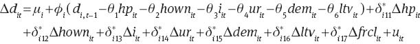
The term in brackets is the long-run relationship between debt and the explanatory variables, while θ1, …, θ6 are the long-run coefficients, which are typically the object of primary interest (see Blackburne III and Frank, 2007). ϕi is the speed of adjustment, which shows what percentage of the gap is being closed in each period and is expected to be negative and significant, if the variables are cointegrated and exhibit a return to long-run equilibrium.
In the long-run, debt at the state level will be determined by:
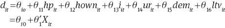
where
As an alternative to our PMG estimator, we also apply the Mean Group (MG) estimator, which estimates independent error-correction equations for each state without imposing homogeneity restrictions on long-run effects, but rather computes the mean of estimated state-specific long-run coefficients. We provide formal statistical evidence for choosing whether our PMG estimator is preferred to the MG estimator by applying a Hausman test on the homogeneity restriction that the long-run coefficient is the same for all states (see Pesaran, Shin, and Smith 1999).
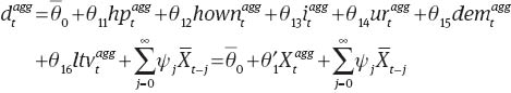
To compute debt in the long run at the aggregate level, we apply the estimated long-run coefficients from the PMG, assumed to be homogeneous, to the US aggregate data:
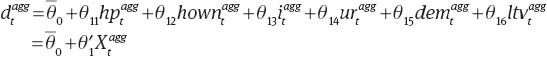
The long-run aggregate constant term
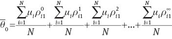
which makes use of
The reason why
As discussed in the main text, the econometric estimation of Equation (5) may be affected by the presence of cross-section dependence across panel members. In what follows, we relax the assumption of cross-section independence of the error term of the standard PMG model by expressing the error term uit as:

where an unspecified number of unobserved common factors ft with idiosyncratic factor loadings λi are allowed to capture time-variant heterogeneity and cross-section dependence, while εit are now idiosyncratic errors independently distributed across i and t. In this set-up, the factors ft can be non-linear and also non-stationary. The regressors Xit are allowed to be driven by some of the same common factors as the dependent variable. We employ two alternative estimators that have been developed to allow for correlation across panel members due to unobserved common time-specific effects as described above: the Augmented Mean Group (AMG) estimator introduced in Eberhardt and Teal (2010) and the Common Correlated Effects Pooled Mean Group (CCEPMG) estimator (see Pesaran 2006; Binder and Offermanns 2007; Chudik and Pesaran 2013).
The basic procedure behind the AMG estimator by Eberhardt and Teal (2010) is described in the main text. The other method used to correct for cross-section dependence in the disturbances is the CCEPMG estimator, which is chosen as our preferred specification when reporting the main results. It is based on the Common Correlated Effects Mean Group (CCEMG) estimator developed by Pesaran (2006). The basic idea is to filter the individual-specific regressors in a way that the differential effects of unobserved common factors are eliminated. The CCEMG solves the problem by augmenting the regressors in the group-specific regression equation with cross-section averages of the dependent variable and the individual-specific regressors.
The focus of the CCEMG estimator is on obtaining consistent estimates of the parameters related to the observable variables, while the estimated coefficients on the cross-section averaged variables are not interpretable in a meaningful way: they are merely present to filter out the biasing impact of the unobservable common factor (see Eberhardt 2012). The CCEMG estimator is robust to the presence of a limited number of “strong” factors (which can represent global shocks, as well as an infinite number of “weak” factors possibly associated with local spillover effects. Moreover, the CCEMG estimator is robust to nonstationary common factors (Kapetanios, Pesaran, and Yamagata 2011) and it continues to hold under slope homogeneity and in the presence of any fixed number of unobserved factors, (see Pesaran 2006).
Augmenting the standard PMG model in Equation (5) with cross-section averages as discussed above, our equation for the CCEPMG estimator becomes:

where
Following (11), the long-run relationship between d and X at the state level is given by:
where
In our final CCEPMG specification, the CCE augmentation of the standard PMG model employs the following cross-section averages (included both in levels and in differences): log of house price to income ratio (hp), unemployment rate (ur), and 35–54 age group (dem).[27]
Based on our final CCEPMG specification, long-run debt at the US aggregate level will be given by:
where
For practical reasons, in the main text we report the estimates for equilibrium debt and debt gaps using the term
B Descriptive statistics and econometric tests
Lag order selection.
| Number of states for which the respective lag order is chosen | Lag order | ||
|---|---|---|---|
| 1 | 2 | 3 | |
| BIC | 26 | 10 | 15 |
| AIC | 1 | 4 | 46 |
BIC and AIC stand respectively for Bayesian and Akaike information criteria.
Descriptive statistics.
| Variable | Obs. | Mean | Std. Dev. | Min | Max |
|---|---|---|---|---|---|
| Total debt to-income ratio | 2856 | 81.3 | 22.2 | 37.7 | 184.1 |
| Log of house price-to-income ratio | 2856 | 1.9 | 0.2 | 1.3 | 2.6 |
| Homeownership rate | 2856 | 69.3 | 6.2 | 37.6 | 82.4 |
| Interest rates | 2856 | 6.1 | 1.0 | 3.6 | 8.5 |
| Unemployment rate | 2856 | 5.7 | 2.1 | 2.2 | 14.1 |
| 35–54 age group | 2856 | 28.7 | 1.7 | 23.0 | 33.3 |
| Loan-to-value ratio | 2856 | 76.0 | 2.0 | 72.1 | 80.4 |
| Foreclosure rate | 2856 | 1.9 | 1.6 | 0.2 | 14.5 |
Source: Bureau of Economic Analysis, Bureau of Labor Statistics, Census Bureau, Federal Housing Finance Agency, Federal Housing Finance Board, FRBNY/Equifax Consumer Credit Panel, Mortgage Bankers Association, and authors’ calculations.
Unit-root tests for variables available at the state level (p-values).
| Debt-to- income ratio | House price-to-income ratio | Homeowner. rate | Interest rate | Unempl. rate | 35–54 age group | |
|---|---|---|---|---|---|---|
| Levin-Lin-Chu | ||||||
| No constant | 1.000 | 0.001 | 0.226 | 0.000 | 0.004 | 0.000 |
| With constant | 0.000 | 1.000 | 0.000 | 1.000 | 0.000 | 1.000 |
| No means | 0.215 | 0.001 | 0.000 | 0.000 | 0.000 | 0.026 |
| Breitung | ||||||
| No constant | 1.000 | 0.001 | 0.228 | 0.000 | 1.000 | 0.000 |
| With constant | 0.962 | 0.416 | 0.000 | 1.000 | 0.867 | 1.000 |
| No means | 0.001 | 0.998 | 0.000 | 0.004 | 0.672 | 1.000 |
| Robust | 0.554 | 0.445 | 0.000 | 0.998 | 0.389 | 1.000 |
| Im-Pesaran-Shin | ||||||
| Uncorr. errors | 0.000 | 1.000 | 0.000 | 1.000 | 1.000 | 1.000 |
| No means | 0.067 | 0.408 | 0.000 | 1.000 | 0.999 | 1.000 |
| Correl. errors | 0.574 | 0.088 | 0.000 | 0.000 | 0.273 | 0.995 |
| Fisher | ||||||
| ADF | 0.001 | 1.000 | 0.066 | 1.000 | 0.129 | 1.000 |
| PP | 0.000 | 1.000 | 0.000 | 1.000 | 1.000 | 1.000 |
| ADF (no means) | 0.865 | 0.133 | 0.000 | 0.000 | 0.624 | 0.997 |
| PP (no means) | 0.254 | 0.422 | 0.000 | 0.463 | 0.808 | 1.000 |
| I(1) at the 1% level | 64% | 79% | 21% | 57% | 79% | 86% |
The tests are based on the null hypothesis that the variables are I(1).
Unit-root tests for variables available at the national level (loan-to-value ratio).
| T-statistic | Critical value at 1% | |
|---|---|---|
| Augmented Dickey-Fuller | ||
| No constant | –0.413 | –2.616 |
| With constant | –1.952 | –3.567 |
| With drift | –1.952 | –2.394 |
| With 3 lags | –2.286 | –3.572 |
| Phillips-Perron | ||
| No constant | –0.391 | –2.616 |
| With constant | –2.145 | –3.567 |
| With trend | –2.132 | –4.130 |
| Kwiatkowski-Phillips- Schmidt-Shin | ||
| Trend stationarity | 0.109 | 0.216 |
| Level stationarity | 0.172 | 0.739 |
| I(1) at the 1% level | 78% | |
The first two tests are based on the null hypothesis that the variable contains a unit root. By contrast, the KPSS test is based on a null hypothesis of stationarity.
Panel cointegration test (τ-bar statistic).
| With constant | With constant and trend | |
|---|---|---|
| Lag order | ||
| 1 | –5.237*** | –5.346*** |
| 2 | –3.978*** | –4.077* |
| 3 | –3.176 | –3.297 |
| 4 | –2.039 | –4.190** |
The test is based on Gengenbach, Urbain, and Westerlund (2009), who have developed a second-generation panel cointegration test that takes into account cross-section dependence. The results test the null hypothesis of no cointegration between the debt-to-income ratio and the five explanatory state-level variables in our error-correction model, with the exception of the loan-to-value ratio which is available only at the national level. The reported lag order is based on the model specification in levels. Asterisks *, ** and *** denote, respectively, significance at the 10%, 5% and 1% levels based on the critical values from Gengenbach, Urbain, and Westerlund (2009), Table 3, p. 31.
Correlation matrix of the cross-sectional averages.
| Avg. house prices | Avg. homeown. | Avg. unempl. | Avg. int. rates | Avg. 35–54 | |
|---|---|---|---|---|---|
| Avg. house prices | 1.00 | ||||
| Avg. homeown. | 0.86 | 1.00 | |||
| Avg. unempl. | –0.32 | –0.50 | 1.00 | ||
| Avg. int. | 0.12 | 0.40 | –0.81 | 1.00 | |
| Avg. 35–54 age | 0.35 | 0.65 | –0.81 | 0.88 | 1.00 |
Source: Bureau of Economic Analysis, Bureau of Labor Statistics, Census Bureau, Federal Housing Finance Agency, Federal Housing Finance Board, FRBNY/Equifax Consumer Credit Panel, Mortgage Bankers Association, and authors’ calculations.
Unit-root tests on the CCEPMG state-level debt gaps.
| p-Values | |
|---|---|
| Levin-Lin-Chu | |
| No constant | 0.000 |
| With constant | 0.000 |
| No means | 0.388 |
| Breitung | |
| No constant | 0.000 |
| With constant | 0.080 |
| No means | 0.006 |
| Robust | 0.208 |
| Im-Pesaran-Shin | |
| Uncorr. errors | 0.000 |
| No means | 0.001 |
| Correl. errors | 0.005 |
| Fisher | |
| ADF | 0.004 |
| PP | 0.000 |
| ADF (no means) | 0.107 |
| PP (no means) | 0.001 |
| I(0) at the 1% level | 71% |
The tests are based on the null hypothesis that the variable contains a unit root.
C Additional tables and figures
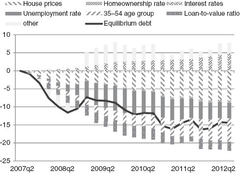
Decomposing the decline in CCEPMG equilibrium debt from 2007Q2.
Source: Authors’ calculations.
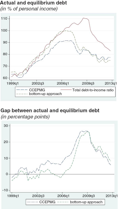
Equilibrium debt and implied gap using a bottom-up approach.
Source: FRBNY/Equifax Consumer Credit Panel and authors’ calculations.
Notes: Equilibrium debt in the bottom-up approach is computed from the aggregation of state-level equilibrium estimates, derived by taking state-weights for income. Last observation refers to 2012Q4.
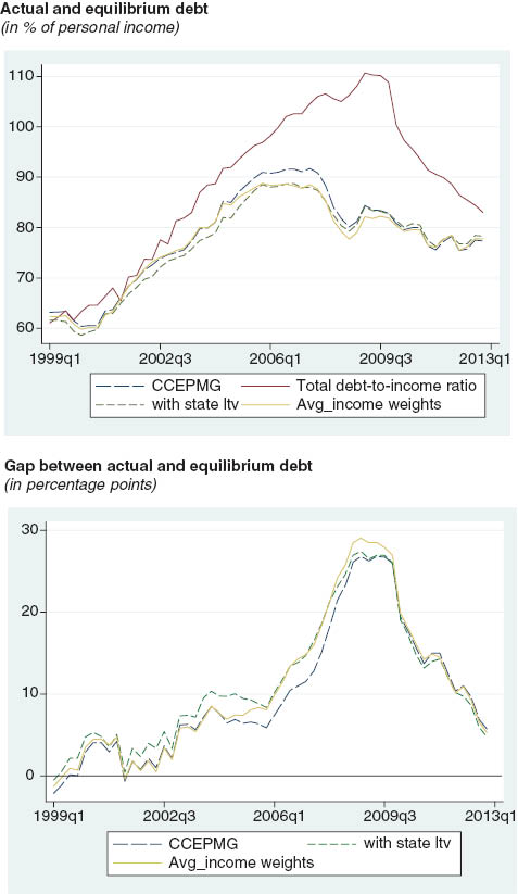
Equilibrium debt and implied gap using the ltv at the state level and weighted cross-sectional averages.
Source: FRBNY/Equifax Consumer Credit Panel and authors’ calculations.
Notes: The “Avg_income weights” specification applies state-income weights to the cross-sectional averages in the CCEPMG. Last observation refers to 2012Q4.
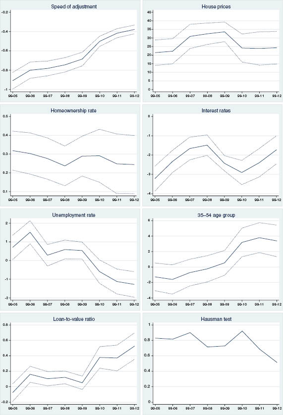
Recursive CCEPMG estimates using different sample periods.
Note: The CCEPMG is estimated recursively over different sample periods: the first estimate considers the 1999–2005 period, and in the subsequent estimates it adds 1 year at a time. The speed of adjustment corresponds to the error correction term in the CCEPMG model. The Hausman test reports p-value under the null hypothesis that the CCEPMG estimator is both efficient and consistent, i.e., that the long-run homogeneity restriction is valid. The remaining solid lines refer to the long-run coefficients on the variables included in the CCEPMG model. Bands around the point estimates consider ± 2 standard errors.
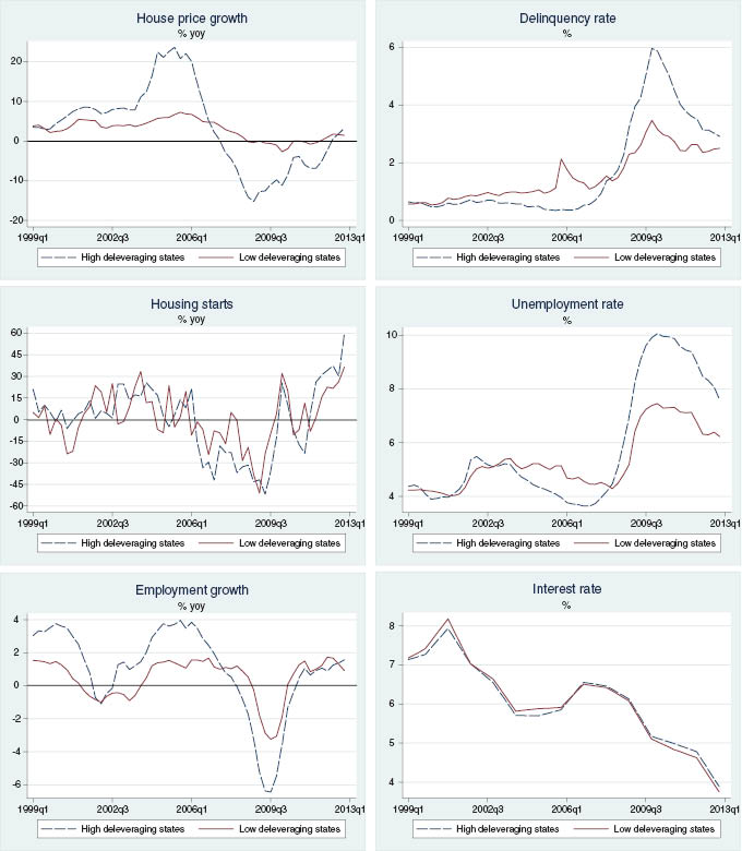
Average developments in economic indicators for high vs. low deleveraging states.
Note: “High deleveraging states” are those states that featured the largest declines in their household debt-to-income ratios between the peak for each state and 2012Q4, defined by the 90th percentile. These include Arizona, California, Florida, Hawaii, Nevada and South Dakota. The “low deleveraging states” are those that featured the smallest declines, defined as the 10th percentile and include Arkansas, Iowa, Kansas, Mississippi, North Dakota and West Virginia.
Sensitivity analysis of CCEPMG model with split samples.
| (1) | (2) | (3) | (4) | (5) | (6) | |
|---|---|---|---|---|---|---|
| CCEPMG | HD states | LD states | HP inter. term | Non-Rec. states | Recourse states | |
| Long-run coefficients | ||||||
| House prices (HP) | 24.320*** | 59.806*** | 19.801*** | 20.417*** | 23.714*** | 20.478*** |
| (4.818) | (16.479) | (7.548) | (5.024) | (7.894) | (5.891) | |
| Homeownership rate | 0.244*** | 0.708** | 0.115 | 0.245*** | 0.069 | 0.326*** |
| (0.079) | (0.336) | (0.095) | (0.079) | (0.121) | (0.094) | |
| Interest rates | –1.727*** | –0.635 | –2.043*** | –1.775*** | –1.195** | –1.836*** |
| (0.370) | (1.221) | (0.516) | (0.369) | (0.609) | (0.440) | |
| Unemployment rate | –1.277*** | –1.085 | –2.391*** | –1.271*** | –1.236* | –1.465*** |
| (0.349) | (1.374) | (0.468) | (0.348) | (0.751) | (0.379) | |
| 35–54 age group | 3.386*** | 9.634** | 3.518*** | 3.269*** | –2.718 | 5.931*** |
| (1.043) | (4.529) | (1.290) | (1.045) | (1.969) | (1.222) | |
| Loan-to-value ratio | 0.526*** | 0.561* | 0.583*** | 0.525*** | 0.457*** | 0.439*** |
| (0.087) | (0.298) | (0.123) | (0.087) | (0.145) | (0.103) | |
| HP*HD states | 46.539*** | |||||
| (16.249) | ||||||
| Speed of Adjustment | –0.378*** | –0.321*** | –0.497*** | –0.380*** | –0.390*** | –0.383*** |
| (0.023) | (0.048) | (0.048) | (0.023) | (0.062) | (0.026) | |
| Half-life | 1.5 | 1.8 | 1 | 1.4 | 1.4 | 1.4 |
| Observations | 2805 | 715 | 715 | 2805 | 660 | 2145 |
| Hausman test (p-value) | 0.513 | 0.998 | 0.637 | 0.52 | 0.535 | 0.655 |
CCEPMG estimates where the dependent variable is household debt-to-income ratio. The lag structure (1 lag) was selected using the Schwartz Bayesian criterion. Foreclosures can only influence household debt in the short run. Standard errors are shown in parentheses. Asterisks, *, **, ***, denote, respectively, statistical significance at the 10, 5 and 1% levels. The half-life estimates indicate the number of quarters it takes to halve the gap between actual and equilibrium debt-to-income ratio. The Hausman test reports p-value under the null hypothesis that the CCEPMG estimator is both efficient and consistent, i.e., that the long-run homogeneity restriction is valid. “High deleveraging states” (HD) stands for the 75th percentile of states with the largest declines in their household debt-to-income ratio from their respective peaks up to 2012Q4, while the “low deleveraging states” (LD) are the 25th percentiles of states with the smallest declines. “Non-recourse states” refer to those states where the lender has no recourse against borrowers if the borrowers’ house is sold at auction or via short sale for less than the amount owned by the lender (Alaska, Arizona, California, Connecticut, Idaho, Minnesota, North Carolina, North Dakota, Oregon, Texas, Utah and Washington, D.C.)
Factor loadings estimates by state.
| State | Deleveraging from peak | Factor loadings | State | Deleveraging from peak | Factor loadings |
|---|---|---|---|---|---|
| Nevada | –81.6 | 2.33* (0.11) | New Mexico | –16.0 | 0.48 (0.03) |
| South Dakota | –55.7 | 1.34* (0.10) | New Jersey | –15.5 | 1.01 (0.03) |
| California | –45.7 | 1.69* (0.06) | Massachusetts | –15.5 | 1.05* (0.02) |
| Arizona | –43.4 | 1.39* (0.05) | Rhode Island | –15.4 | 1.10* (0.04) |
| Florida | –36.8 | 1.28* (0.06) | Tennessee | –15.3 | 0.73 (0.02) |
| Hawaii | –36.3 | 0.84 (0.10) | New York | –15.0 | 0.75 (0.02) |
| Oregon | –28.1 | 1.24* (0.03) | Delaware | –14.8 | 1.36* (0.06) |
| Maine | –26.4 | 0.93 (0.03) | Nebraska | –14.5 | 0.73 (0.02) |
| Vermont | –25.9 | 1.03 (0.04) | Texas | –13.5 | 0.45 (0.02) |
| Georgia | –24.8 | 1.29* (0.03) | Wisconsin | –13.1 | 0.75 (0.01) |
| Colorado | –24.1 | 1.23* (0.06) | Missouri | –12.4 | 0.72 (0.02) |
| Washington | –23.6 | 0.98 (0.03) | Pennsylvania | –12.3 | 0.63 (0.01) |
| Maryland | –23.3 | 1.12* (0.02) | Distr. of Columbia | –11.9 | 0.63 (0.05) |
| Michigan | –23.0 | 1.13* (0.03) | Alabama | –11.3 | 0.64 (0.03) |
| Virginia | –22.5 | 1.16* (0.02) | Kentucky | –10.8 | 0.78 (0.01) |
| New Hampshire | –21.0 | 1.23* (0.04) | Louisiana | –10.2 | 0.37 (0.03) |
| Wyoming | –19.8 | 0.50 (0.06) | Alaska | –10.1 | 0.56 (0.04) |
| Illinois | –19.5 | 1.02 (0.02) | Montana | –10.0 | 0.59 (0.03) |
| Idaho | –17.7 | 1.07 (0.04) | Oklahoma | –9.3 | 0.46 (0.02) |
| Ohio | –17.2 | 0.78 (0.04) | Kansas | –7.4 | 0.55 (0.02) |
| Minnesota | –17.1 | 0.99 (0.02) | Arkansas | –7.1 | 0.58 (0.02) |
| Utah | –17.1 | 0.80 (0.04) | North Dakota | –6.4 | 0.26 (0.01) |
| Indiana | –16.7 | 0.88 (0.03) | Mississippi | –6.3 | 0.56 (0.03) |
| North Carolina | –16.6 | 0.92 (0.02) | Iowa | –3.9 | 0.85 (0.02) |
| South Carolina | –16.5 | 0.70 (0.04) | West Virginia | –3.0 | 0.36 (0.04) |
| Connecticut | –16.0 | 0.87 (0.02) |
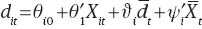
The figures on the column with the factor loadings refer to the slope coefficients obtained from regressing the debt gap of each state on the difference between average debt and the averages of the explanatory variables, which stands as a proxy for the unobserved common factor(s). More precisely, we estimate
References
Aron, J., and J. Muellbauer. 2013. “Wealth, Credit Conditions and Consumption: Evidence from South Africa.” Review of Income and Wealth 59: S161–S196.Suche in Google Scholar
Arpaia, A., and A. Turrini. 2008. “Government Expenditure and Economic Growth in the EU: Long-Run Tendencies and Short-Term Adjustment.” European Economy Economic Papers 300.10.2139/ssrn.1097286Suche in Google Scholar
Barba, A., and M. Pivetti. 2009. “Rising Household Debt: Its Causes and Macroeconomic Implications–A Long-Period Analysis.” Cambridge Journal of Economics 33: 113–137.10.1093/cje/ben030Suche in Google Scholar
Barnes, S., and G. Young. 2003. “The Rise in US Household Debt: Assessing its Causes and Sustainability.” Bank of England Working Paper, 206.Suche in Google Scholar
Binder, M., and G. Offermanns. 2007. “International Investment Positions and Exchange Rate Dynamics: A Dynamic Panel Analysis.” CFS Working Paper, 2007/23.Suche in Google Scholar
Blackburne III, E., and M. Frank. 2007. “Estimation of Nonstationary Heterogeneous Panels.” The Stata Journal 7 (2): 197–208.10.1177/1536867X0700700204Suche in Google Scholar
Brown, M., A. Haughwout, D. Lee, and W. van der Klaauw. 2010. “The Financial Crisis at the Kitchen Table: Trends in Household Debt and Credit.” Federal Reserve Bank of New York Staff Report, 480.Suche in Google Scholar
Chudik, A., and M. Pesaran. 2013. “Common Correlated Effects Estimation of Heterogeneous Dynamic Panel Data Models with Weakly Exogenous Regressors.” Federal Reserve Bank of Dallas Working Paper, No. 146.Suche in Google Scholar
Chudik, A., H. Pesaran, and E. Tosetti. 2011. “Weak and Strong Cross-Section Dependence and Estimation of Large Panels.” The Econometrics Journal 14 (1): C45–C90.10.1111/j.1368-423X.2010.00330.xSuche in Google Scholar
Csonto, B., and I. Ivaschenko. 2013. “Determinants of Sovereign Bond Spreads in Emerging Markets: Local Fundamentals and Global Factors vs. Ever-Changing Misalignments.” IMF Working Paper, 164.10.5089/9781475573206.001Suche in Google Scholar
Cuerpo, C., I. Drumond, J. Lendvai, P. Pontuch, and R. Raciborski. 2013. “Indebtedness, Deleveraging Dynamics and Macroeconomic Adjustment.” European Economy Economic Papers, 477.Suche in Google Scholar
Durdu, C., E. Mendoza, and M. Terrones. 2013. “On the Solvency of Nations: Cross-Country Evidence on the Dynamics of External Adjustment.” Journal of International Money and Finance 32: 762–780.10.1016/j.jimonfin.2012.07.002Suche in Google Scholar
Dynan, K. 2012. Is a Household Debt Overhang Holding Back Consumption? Brookings Papers on Economic Activity. Spring.10.2139/ssrn.2132615Suche in Google Scholar
Dynan, K., and D. Kohn. 2007. “The Rise in US Household Indebtedness: causes and consequences. Board of Governors of the Federal Reserve System.” Finance and Economics Discussion Series 37.10.17016/FEDS.2007.37Suche in Google Scholar
Eberhardt, M. 2012. “Estimating Panel Time Series Models with Heterogeneous Slopes.” The Stata Journal 12 (1): 61–71.10.1177/1536867X1201200105Suche in Google Scholar
Eberhardt, M., and F. Teal. 2010. “Productivity Analysis in Global Manufacturing Production.” University of Oxford, Economics Series Working Papers, 515.Suche in Google Scholar
Eberhardt, M., and F. Teal. 2013a. “No Mangoes in the Tundra: Spatial Heterogeneity in Agricultural Productivity Analysis.” Oxford Bulletin of Economics and Statistics 75 (6): 914–939.10.1111/j.1468-0084.2012.00720.xSuche in Google Scholar
Eberhardt, M., and F. Teal. 2013b. “Structural Change and Cross-Country Growth Empirics.” The World Bank Economic Review 27 (2): 229–271.10.1093/wber/lhs020Suche in Google Scholar
Edelberg, W. 2003. “Risk-Based Pricing of Interest Rates in Household Loan Markets. Board of Governors of the Federal Reserve System.” Finance and Economics Discussion Series, 62.Suche in Google Scholar
Egert, B., A. Lahreche-Revil, and K. Lommatzsch. 2004. “The Stock-Flow Approach to the Real Exchange Rate of CEE Transition Economies.” CEPII Working Paper, 15.Suche in Google Scholar
Eggertsson, G., and P. Krugman. 2012. “Debt, Deleveraging, and the Liquidity Trap: A Fisher-Minsky-Koo Approach.” The Quarterly Journal of Economics 127 (3): 1469–1513.10.1093/qje/qjs023Suche in Google Scholar
Emmons, W., and B. Noeth. 2013. “Online Extra: Mortgage Borrowing: The Boom and Bust.” Federal Reserve Bank of St. Louis – The Regional Economist,January 2013.Suche in Google Scholar
Fernandez-Corugedo, E., and J. Muellbauer. 2006. “Consumer Credit Conditions in the United Kingdom.” Bank of England Working Paper, 314.Suche in Google Scholar
Finocchiaro, D., C. Nilsson, D. Nyberg, and A. Soultanaeva. 2011. “Household Indebtedness, House Prices and the Macroeconomy: A Review of the Literature.” Sveriges Riksbank Economic Review 1: 6–28.Suche in Google Scholar
Gengenbach, C., J.-P. Urbain, and J. Westerlund. 2009. “Panel Error Correction Testing with Global Stochastic Trends.” Research Memoranda, METEOR, Maastricht Research School of Economics of Technology and Organization, 051.Suche in Google Scholar
Holly, S., M. Pesaran, and T. Yamagata. 2010. “A Spatio-Temporal Model of House Prices in the USA.” Journal of Econometrics 158 (1): 160–173.10.1016/j.jeconom.2010.03.040Suche in Google Scholar
Iacoviello, M. 2004. “Consumption, House Prices, and Collateral Constraints: A Structural Econometric Analysis.” Journal of Housing Economics 13: 304320.Suche in Google Scholar
Kapetanios, G., M. Pesaran, and T. Yamagata. 2011. “Panels with Nonstationary Multifactor Error Structures.” Journal of Econometrics 160 (2): 326–348.10.1016/j.jeconom.2010.10.001Suche in Google Scholar
Kiss, G., N. Márton, and B. Vonnák. 2006. “Credit Growth in Central and Eastern Europe: Convergence or Boom?” MNB Working Papers, 10.Suche in Google Scholar
Kiyotaki, N., and J. Moore. 1997. “Credit Cycles.” Journal of Political Economy 105 (2): 211–248.10.1086/262072Suche in Google Scholar
Koo, R. 2008. The Holy Grail of Macroeconomics – Lessons from Japan’s Great Recession. New York: John Wiley & Sons.Suche in Google Scholar
Koo, R. 2013. “Balance Sheet Recession as the “Other Half” of Macroeconomics.” European Journal of Economics and Economic Policies: Intervention 10 (2): 136–157.10.4337/ejeep.2013.02.01Suche in Google Scholar
Mayer, C., and K. Pence. 2008. “Subprime Mortgages: What, Where, and to Whom? Board of Governors of the Federal Reserve System.” Finance and Economics Discussion Series, 29.Suche in Google Scholar
McKinsey Global Institute. 2012. “Debt and Deleveraging: Uneven Progress on the Path to Growth”. McKinsey Global Institute Report, January 2012.Suche in Google Scholar
Mian, A., and A. Sufi. 2010. “Household Leverage and the Recession of 2007–2009.” IMF Economic Review 58 (1): 74–117.10.1057/imfer.2010.2Suche in Google Scholar
Mian, A., K. Rao, and A. Sufi. 2013. “Household Balance Sheets, Consumption, and the Economic Slump.” The Quarterly Journal of Economics 128 (4): 1687–1726.10.1093/qje/qjt020Suche in Google Scholar
Nieto, F. 2007. “The Determinants of Household Credit in Spain.” Banco de Espana Documentos de Trabajo, 0716.Suche in Google Scholar
Pesaran, H., R. Smith, and K. Im. 1996. “Dynamic Linear Models for Heterogeneous Panels.” In The Econometrics of Panel Data, edited by L. Mtys and P. Sevestre. Dordrecht: Kluwer Academic Publishers.10.1007/978-94-009-0137-7_8Suche in Google Scholar
Pesaran, M. 2004. “General Diagnostic Tests for Cross Section Dependence in Panels.” CESifo Working Paper Series, No. 1229.Suche in Google Scholar
Pesaran, M. 2006. “Estimation and Inference in Large Heterogeneous Panels with a Multifactor Error Structure.” Econometrica 74 (4): 9671012.10.1111/j.1468-0262.2006.00692.xSuche in Google Scholar
Pesaran, M., and Y. Shin. 1999. “An Autoregressive Distributed Lag Modelling Approach to Cointegration Analysis.” In Econometrics and Economic Theory in the 20th Century: The Ragnar Frisch Centennial Symposium, edited by Steinar Strøm. Cambridge: Cambridge University Press.Suche in Google Scholar
Pesaran, M., Y. Shin, and R. Smith. 1999. “Pooled Mean Group Estimation of Dynamic Heterogeneous Panels.” Journal of the American Statistical Association 94 (446): 621–634.10.1080/01621459.1999.10474156Suche in Google Scholar
Poghosyan, T. 2012. “Long-Run and Short-Run Determinants of Sovereign Bond Yields in Advanced Economies.” IMF Working Paper, 271.Suche in Google Scholar
Rajan, R. 2010. Fault Lines: How Hidden Fractures Still Threaten The World Economy. Princeton: Princeton University Press.10.1515/9781400839803Suche in Google Scholar
Roberts, L. 2008. The Great Housing Bubble-Why Did House Prices Fall? Las Vegas: Monterey Cypress Publishing.Suche in Google Scholar
Schmitt, E. 2000. “Does Rising Consumer Debt Signal Future Recessions?: Testing the Causal Relationship Between Consumer Debt and the Economy.” Atlantic Economic Journal 28 (3): 333–345.10.1007/BF02298325Suche in Google Scholar
Wyplosz, C. 2007. “Debt Sustainability Assessment: The IMF Approach and Alternatives.” HEI Working Paper, 03.Suche in Google Scholar
©2015 by De Gruyter
Artikel in diesem Heft
- Frontmatter
- Advances
- Consumption composition and macroeconomic dynamics
- Evaluating linear approximations in a two-country model with occasionally binding borrowing constraints
- Contributions
- The bank lending channel and monetary policy rules for Eurozone banks: further extensions
- Investment lags and macroeconomic dynamics
- The zero lower bound: frequency, duration, and numerical convergence
- What drives endogenous growth in the United States?
- Environmental policy and economic growth: the macroeconomic implications of the health effect
- US household deleveraging following the Great Recession – a model-based estimate of equilibrium debt
- Price-level instability and international monetary policy coordination
- Households forming macroeconomic expectations: inattentive behavior with social learning
- Topics
- Complementarity and transition to modern economic growth
- Trend inflation and monetary policy rules: determinacy analysis in New Keynesian model with capital accumulation
- Discussions
- Preface to “Reflections on Macroeconometric Modeling” by Ray C. Fair
- Reflections on macroeconometric modeling