Evaluating linear approximations in a two-country model with occasionally binding borrowing constraints
-
Alexis Anagnostopoulos
 und
Xin Tang
und
Xin Tang

Abstract
Under a linear approximation, a standard two-country business cycles model with incomplete markets delivers consumption and debt dynamics that are non-stationary (unit root) and a bond price that is independent of the wealth distribution. We argue that these two features are due to the local nature of the approximation and we show that they survive even when second or third order local approximations are used. However, these features disappear when debt limits and the associated precautionary motives are taken into account by a standard, global solution method. We subsequently investigate whether this qualitative difference has significant quantitative implications regarding the linear solution as an approximation to the model’s equilibrium dynamics. Policy function differences between the local and global solutions can be large and remain significant even in the case of debt limits as loose as the natural debt limit. These differences can lead to significant discrepancies in implied simulated second moments. In a benchmark calibration, the cross-country correlation of consumption is 0.61 under linearization, but only 0.38 when a policy iteration algorithm is used.
Acknowledgments
We have greatly benefited from suggestions, discussions and comments by Wouter den Haan, Albert Marcet and Morten Ravn. We also wish to acknowledge helpful comments made by Eva Carceles-Poveda, Tom Muench, Tom Sargent, Andrew Scott, Kjetil Storesletten and participants at the X Workshop on Dynamic Marcoeconomics in Vigo, Spain.
Alexis Anagnostopoulos wishes to acknowledge financial support from the European Commission, MAPMU network under contract HPRN-CT-2002-00237.
Appendix A Perturbation methods
In this appendix, we provide the first order approximation of the policy functions in the more general case where the point of approximation is chosen to be
The first order approximation is given by
where BLIN, CLIN and PLIN represent the policy functions for country 1’s bonds, consumption and for equilibrium prices, respectively. The coefficients By1, By2, Py, Cy1 and Cy2 represent the derivative of the corresponding true function with respect to the variable indicated in the subscript, evaluated at the steady state. These derivatives are given in terms of the parameters in what follows
Note that the bond law of motion has a unit root regardless of the assumptions on utility and of the steady state bond level
Appendix B Policy iteration method
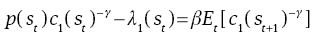
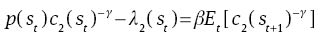
This appendix provides a brief description of the policy iteration algorithm used and the parameter choices made. The equilibrium conditions that need to be satisfied at every possible state of the economy st=(y1t, y2t, b1t–1) are
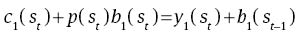
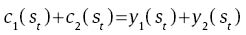
Note that the bond market clearing condition has already been used to substitute out b2(st)=–b1(st) and the budget constraint for country 2 is omitted since it is automatically satisfied by Walras’ law. All variables are expressed as functions of the state vector st. As discussed in Ljungqvist and Sargent (2004), and contrary to the complete markets case, the equilibrium is not recursive in the exogenous state variables (y1t, y2t). That is, the wealth redistribution needs to be added as a state variable given the incompleteness of financial markets. Because the current model consists of only two agents, adding the variable b1 to the state vector is enough to keep track of the wealth distribution. Note that exogenous income is trivially dependent on the state vector as y1(st)=y1t and y2(st)=y2t.
The first step is to discretize the state space. The AR(1) process given in (2) is approximated with a Markov chain with M=9 states for each shock, implying a total of M2=81 states for the two shocks together. The discretization procedure follows the method of Tauchen and Hussey (1991) adjusted as suggested in Flodén (2008) to improve its performance for processes with high level of persistence. The resulting Markov chain has values for persistence and variance that match the corresponding ρ and
The endogenous state variable (bond) lies in an interval [–K, K] where K=1 is the debt limit. This interval is discretized using N=301 points with higher concentration of points closer to the limits (points are distributed according to a quadratic function). Although 301 points is not a very large number, Euler errors end up being relatively small. This is to a large extent due to the use of interpolation for the space in between points. In the case of loose limits (K=80.7) we use N=3000 to accommodate the fact that the state space is much wider.
To summarize up to now, we have obtained a collection of M2N points in the state space. From here on we drop the time subscripts and denote the current state at a point i in the grid by si=(b1j, y1k, y2r), i∈{(j, k, r):j=1, …, N, k=1, …, M, r=1, …, M}. Also let s and s′ denote a generic value for the current and future state vectors, respectively. Given guesses
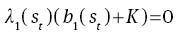
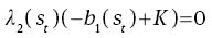
Assume limits do not bind at si=(b1j, y1k, y2r) so that Λ1(si)=Λ2(si)=0. Using (B1)–(B4), straightforward algebra gives
If B1(si)<–K, then set
If B1(si)>K, then set
It is not possible to obtain closed form expressions in cases 2 and 3, so a non-linear equation solver is used to obtain a solution numerically. When this procedure is finished for all points s in the state space, we have implied policy functions
Appendix C Euler errors
This appendix provides accuracy measures for our policy iteration method as well as for the perturbation methods. We show that Euler errors are small for our global solution which supports the claim in the main text that the policy function differences between the global solution and the perturbation methods are not due to inaccuracy in the global method.
C.1 Static Euler errors
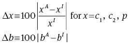
Euler errors, as suggested by Judd (1992) and described in more detail in den Haan (2010), are a widely used measure of the accuracy of numerical solutions of dynamic models. The policy iteration algorithm delivers policy functions which satisfy the Euler equations (up to the tolerance level used for algorithm convergence, in our case 10–11) at the points in the state space chosen during the discretization procedure. The idea is to check the size of the approximation error at other points in the state space. We look at the midpoints lying in between discretization points and calculate the Euler equation errors at these points. Specifically, at each point we use our (linearly interpolated) policy functions to obtain “actual” values for current consumption, bonds and prices. We then compare these to the “implied” values obtained by directly solving the non-linear equations (3)–(8) for cit, b1t, pt with the conditional expectations calculated using our policy functions.[20] Santos (2000) shows that these Euler errors can be used to evaluate the accuracy of the solution since their size is closely related to the distance of the approximated policy functions to the true solution.[21] For each variable x=c1, c2, b1, p, we compute the absolute difference between actual values xA and implied values xI at each point considered. We express this difference as a percentage of xI for x=c1, c2, p and as a fraction of mean income for bonds b, and denote them by Δx
Tables 6 and 7 reports the Euler errors for the benchmark calibration.
Static Euler errors, policy iteration solution.
| Whole state space | Binding points excluded | |||
|---|---|---|---|---|
| Max | Mean | Max | Mean | |
| Δc | 0.0077% | 1.82×10⁻⁵% | 0.0026% | 1.90×10⁻⁵% |
| Δb | 0.0129% | 2.11×10⁻⁵% | 0.0024% | 1.89×10⁻⁵% |
| Δp | 0.0063% | 0.30×10⁻⁵% | 0.90×10⁻⁵% | 4.90×10⁻⁸% |
Static Euler errors, linear solution.
| Whole state space | Binding points excluded | |||
|---|---|---|---|---|
| Max | Mean | Max | Mean | |
| Δc | 3.86% | 0.530% | 0.041% | 0.009% |
| Δb | 6.69% | 1.042% | 0.237% | 0.082% |
| Δp | 3.13% | 0.502% | 0.102% | 0.037% |
The maximum and the average values of these are reported in Table 6. Euler errors are of similar order of magnitude for the three variables, so we focus on consumption. At most points in the state space Euler errors are very small, as indicated by the average being 1.8×10⁻⁵%. Euler errors are larger close to the limits, with the maximum at 0.0077% of consumption. Overall, we find the errors to be reasonably small and, importantly, several orders of magnitude smaller than the differences between linear and policy iteration solutions reported in the previous section. This provides some confidence that the differences reported in section 4.3 of the main text are not simply due to large approximation errors in the policy iteration solution.
We have also computed Euler errors for the linear solution which we present in Table 7. Focusing on consumption, maximum Euler errors are almost 4% of consumption and average errors are 0.53%. These are several orders of magnitude higher than the policy iteration errors. The maximum error is of similar size to the maximum policy difference, but the average errors appear to be smaller than what the policy differences would suggest. Indeed, when we exclude the limit points, the maximum falls to 0.04% of consumption and the average is approximately 0.01% of consumption. Although still significantly larger than the PI solution errors, these could be argued to be reasonably small for a first approximation and they paint a very different picture than what policy differences would suggest. We interpret this as evidence of the importance of the expectations of future binding constraints, even when constraints do not currently bind. Whereas the global approximation method builds this in the conditional expectations, the linear solution does not. When computing standard Euler errors for the linear solution, we compute conditional expectations using the linear policy, i.e., ignoring the possibility of future binding constraints. Under this assumption, current actual decisions are not too far away from the implied ones. But the global solution is actually very different exactly because these expectations are very different. Thus, focusing on Euler errors can be misleading as a measure of the quality of approximation obtained with linear methods for a model with occasionally binding constraints, even if one focuses on points that are away from the limits.
The Euler errors of the solutions under the natural debt limit are presented in Table 8.
Static Euler errors, with K=80.7 and γ=1.
| Policy iteration | First order | Second order | ||||
|---|---|---|---|---|---|---|
| Max | Mean | Max | Mean | Max | Mean | |
| Δc | 0.293% | 1.76×10⁻⁷% | 3.50% | 0.014% | 5.43% | 0.012% |
| Δb | 0.060% | 2.54×10⁻⁷% | 17.20% | 0.794% | 10.75% | 0.377% |
| Δp | 0.0007% | 2.44×10⁻⁹% | 0.131% | 0.018% | 0.141% | 0.0173% |
C.2 Dynamic Euler errors
den Haan (2010) suggests a second accuracy measure which he terms dynamic Euler errors, as opposed to the static Euler errors computed in the previous section. The idea is to evaluate whether small static Euler errors can accumulate to large errors in a simulation. This is especially relevant for our case, since we know that the linear solution yields non-stationary policy functions so one of the main concerns about its accuracy is exactly this accumulation of errors in a simulation.
To produce a simulated series, we first draw a sequence of realizations for the exogenous income shocks and initialize the series at the steady state values for the state variables. For the “actual” series, we use directly the policy functions in each period to compute values for bonds, consumptions and prices given the exogenous shock. The bond choice at t is then the state variable for t+1 and a simulation is produced recursively. For the “implied” series, we compute current values by evaluating expectations according to the policy function but directly solving the non-linear equilibrium conditions for current bonds, consumptions and prices. This implied value for the bond choice at t is then used as the state variable for t+1 and the simulation is thus produced recursively again. In order to focus on the possibility of future binding constraints we produce many short run simulations as opposed to one very long one. This is intended to give the linear solution the best chance to perform well. In a very long simulation, the unit root in the linear bond law of motion would imply bonds that drift arbitrarily far away from the steady state and, in particular, above the limits. We choose the simulation length to be 50 periods and compute average errors over 20,000 repetitions. The draws of the exogenous shocks are kept the same in the simulations using the linear and global solution to make those directly comparable.
We define Δx as in (C7) and report these dynamic Euler errors for the policy iteration method in the top panel of Table 9. It is important to note that the limits never bind in any of the simulations. This is partly due to the fact that the debt policy function is mean-reverting but also due to the fact that we are looking at short run simulations starting at zero bonds. The errors are thus small because the static Euler errors away from the limits are small and there does not seem to be substantial accumulation of errors in a 50 period simulation. The maximum consumption error occurs when bonds come close to the limit and is 0.0022%. The economy spends most of these simulations far from the limits so the average is very small at 3.74×10⁻⁶%. The corresponding statistics for the linear solution are shown in the bottom panel of Table 9. Despite the short simulation length, in the linear equilibrium debt sometimes reaches the debt limits. In the implied series, this limit is imposed but in the actual series it is not, since the linear policies do not assume such limits. As a result, the maximum error in bonds can be extremely high, indeed it can be arbitrarily high if we increase the simulation length.[22] For our short simulation experiment, this only happens for <2% of the periods. For consumption, the maximum error is more than 3% of consumption and the average is 0.033%. Consumption errors are significantly smaller than errors in bonds because of a moderating effect from prices. In the implied allocations, when bonds cannot adjust due to the limits, prices increase significantly, sometimes rising even above one. This provides significant consumption smoothing for the borrowing constrained country, keeping the consumption allocations from diverging even further away from the ones in the actual simulation.
Dynamic Euler errors.
| Max | Mean | |
|---|---|---|
| Policy iteration solution | ||
| Δc | 0.0022% | 3.74×10⁻⁶% |
| Δb | 0.0028% | 7.08×10⁻⁵% |
| Δp | 8.24×10⁻⁷% | 9.75×10⁻⁹% |
| Linear solution | ||
| Δc | 3.86% | 0.033% |
| Δb | 140.25% | 0.50% |
| Δp | 3.13% | 0.041% |
To sum up, Euler errors can accumulate significantly for bonds as they drift above the limits, but this does not necessarily translate to large accumulation of errors for consumption, partly because prices adjust to provide some consumption smoothing. Before the limits are reached, actual and implied series stay very close even for the linear solution, indicating small dynamic Euler errors as long as the limits don’t bind in the simulation. Similarly to the previous section, we note that the use of the linear policies to evaluate expectations essentially shuts down any effects from the possibility of future binding constraints. As a result, small dynamic Euler errors for the linear solution does not necessarily imply that the dynamic properties of the linear economy match well with those of the non-linear economy with constraints. This point is illustrated by the cross-country consumption correlations reported in the main text.
References
Aiyagari, S. R. 1994. “Uninsured Idiosyncratic Risk and Aggregate Saving.” The Quarterly Journal of Economics 109: 659–684.10.2307/2118417Suche in Google Scholar
Backus, D. K., P. J. Kehoe, and F. E. Kydland. 1992. “International Real Business Cycles.” Journal of Political Economy 100: 745–775.10.1086/261838Suche in Google Scholar
Baxter, M. 1995. “International Trade and Business Cycles.” In Handbook of International Economics, vol. 3, chap. 35, 1801–1864, 1 ed. edited by G. M. Grossman and K. Rogoff. Amsterdam, The Netherlands: Elsevier/North-Holland.10.1016/S1573-4404(05)80015-2Suche in Google Scholar
Baxter, M., and M. J. Crucini. 1995. “Business Cycles and the Asset Structure of Foreign Trade.” International Economic Review 36: 821–854.10.2307/2527261Suche in Google Scholar
Blanchard, O. J., and C. M. Kahn. 1980. “The Solution of Linear Difference Models under Rational Expectations.” Econometrica 48: 1305–1311.10.2307/1912186Suche in Google Scholar
Carroll, C. D., and M. S. Kimball. 1996. “On the Concavity of Consumption Function.” Econometrica 64: 981–992.10.2307/2171853Suche in Google Scholar
Carroll, C. D., and M. S. Kimball. 2001. “ Liquidity Constraints and Precautionary Saving.” NBER Working Paper 8496.10.3386/w8496Suche in Google Scholar
Christiano, L. J. 1990. “Solving the Stochastic Growth Model by Linear-Quadratic Approximation and by Value-Function Iterations.” Journal of Business and Economic Statistics 8: 23–26.Suche in Google Scholar
Christiano, L. J. 2002. “Solving Dynamic Equilibrium Models by a Method of Undetermined Coefficients.” Computational Economics 20: 21–55.10.1023/A:1020534927853Suche in Google Scholar
Coleman, W. J. I. 1990. “Solving the Stochastic Growth Model by Policy-Function Iteration.” Journal of Business & Economic Statistics 8: 27–29.10.1080/07350015.1990.10509769Suche in Google Scholar
Deaton, A. 1991. “Saving and Liquidity Constraints.” Econometrica 59: 1221–1248.10.2307/2938366Suche in Google Scholar
den Haan, W. J. 2001. “The Importance of the Number of Different Agents in a Heterogeneous Asset-Pricing Model.” Journal of Economic Dynamics and Control 25: 721–746.10.1016/S0165-1889(00)00038-5Suche in Google Scholar
den Haan, W. J. 2010. “Comparison of Solutions to the Incomplete Markets Model with Aggregate Uncertainty.” Journal of Economic Dynamics and Control 34: 4–27.10.1016/j.jedc.2008.12.010Suche in Google Scholar
Flodén, M. 2008. “A Note on the Accuracy of Markov-Chain Approximations to Highly Persistent AR(1) Process.” Economic Letters 99: 516–520.10.1016/j.econlet.2007.09.040Suche in Google Scholar
Granger, C. W. J., and N. R. Swanson. 1997. “An Introduction to Stochastic Unit-Root Process.” Journal of Econometrics 80: 35–62.10.1016/S0304-4076(96)00016-4Suche in Google Scholar
Heaton, J., and D. J. Lucas. 1996. “Evaluating the Effects of Incomplete Markets on Risk Sharing and Assets Pricing.” Journal of Political Economy 104: 443–487.10.1086/262030Suche in Google Scholar
Huggett, M. 1993. “The Risk-free Rate in Heterogeneous-agent Incomplete-insurance Economies.” Journal of Economic Dynamics and Control 17: 953–969.10.1016/0165-1889(93)90024-MSuche in Google Scholar
Judd, K. L. 1992. “Projection Methods for Solving Aggregate Growth Models.” Journal of Economic Theory 58: 410–452.10.1016/0022-0531(92)90061-LSuche in Google Scholar
Judd, K. L. 1998. Numerical Methods in Economics. Cambridge, Massachusetts and London, England: MIT Press.Suche in Google Scholar
Kehoe, P. J., and F. Perri. 2002. “International Business Cycles with Endogenous Incomplete Markets.” Econometrica 70: 907–928.10.1111/1468-0262.00314Suche in Google Scholar
Kimball, M. S. 1990. “Precautionary Saving in the Small and in the Large.” Econometrica 58: 53–73.10.2307/2938334Suche in Google Scholar
King, R. G., C. I. Plosser, and S. T. Rebelo. 1988. “Production, Growth and Business Cycles: 1. The Basic Neoclassical Model.” Journal of Monetary Economics 21: 195–232.10.1016/0304-3932(88)90030-XSuche in Google Scholar
Kollman, R. 1996. “Incomplete Asset Markets and the Cross-Country Consumption Correlation Puzzle.” Journal of Economic Dynamics and Control 20: 945–961.10.1016/0165-1889(95)00883-7Suche in Google Scholar
Lane, P. R., and G. M. Milesi-Ferretti. 2007. “The External Wealth of Nations mark II: Revised and Extended Estimates of Foreign Assets and Liabilities, 1970–2004.” Journal of international Economics 73: 223–250.10.1016/j.jinteco.2007.02.003Suche in Google Scholar
Levine, D. K., and W. R. Zame. 1996. “Debt Constraints and Equilibrium in Infinite Horizon Economies with Incomplete Markets.” Journal of Mathematical Economics 26: 103–131.10.1016/0304-4068(95)00745-8Suche in Google Scholar
Ljungqvist, L., and T. J. Sargent. 2004. Recursive Macroeconomic Theory, 2nd ed. Cambridge, Massachusetts and London, England: MIT Press.Suche in Google Scholar
Magill, M., and M. Quinzii. 1994. “Infinite Horizon Incomplete Markets.” Econometrica 62(4): 853–880.10.2307/2951735Suche in Google Scholar
Marcet, A., and A. Scott. 2009. “Debt and Deficit Fluctuations and the Structure of Bond Markets.” Journal of Economic Theory 144: 473–501.10.1016/j.jet.2008.06.009Suche in Google Scholar
Marcet, A., and K. J. Singleton. 1999. “Equilibrium Asset Prices and Savings of Heterogeneous Agents in the Presence of Incomplete Markets and Portfolio Constraints.” Macroeconomic Dynamics 3: 243–277.10.1017/S1365100599011062Suche in Google Scholar
Mcgrattan, E. R. 1990. “Solving the Stochastic Growth Model by Linear-Quadratic Approximation.” Journal of Business and Economic Statistics 8: 41–44.Suche in Google Scholar
Petrosky-Nadeau, N., and L. Zhang. 2013. “Solving the DMP Model Accurately.” NBER Working Paper.10.3386/w19208Suche in Google Scholar
Rendahl, P. 2014. “Inequality Constraints and Euler Equation Based Solution Methods.” Economic Journal. DOI: 10.1111/ecoj.12115.10.1111/ecoj.12115Suche in Google Scholar
Santos, M. S. 2000. “Accuracy of Numerical Solutions Using the Euler Equation Residuals.” Econometrica 68: 1377–1402.10.1111/1468-0262.00165Suche in Google Scholar
Schmitt-Grohé, S., and M. Uribe. 2003. “Closing Small Open Economy Models.” Journal of International Economics 61: 163–185.10.1016/S0022-1996(02)00056-9Suche in Google Scholar
Schmitt-Grohé, S., and M. Uribe. 2004. “Solving Dynamic General Equilibrium Models using a Second-Order Approximation to the Policy Function.” Journal of Economic Dynamics and Control 28: 755–775.10.1016/S0165-1889(03)00043-5Suche in Google Scholar
Tauchen, G. 1986. “Finite State Markov-chain Approximations to Univariate and Vector Autoregressions.” Economic Letters 20: 177–181.10.1016/0165-1765(86)90168-0Suche in Google Scholar
Tauchen, G., and R. Hussey. 1991. “Quadrature-Based Methods for Obtaining Approximate Solutions to Nonlinear Asset Pricing Models.” Econometrica 59: 371–396.10.2307/2938261Suche in Google Scholar
Telmer, C. I. 1993. “Assets-Pricing Puzzles and Incomplete Markets.” The Journal of Finance 48: 1803–1832.10.1111/j.1540-6261.1993.tb05129.xSuche in Google Scholar
Uhlig, H. 1999. “A Toolkit for Analyzing Non-linear Dynamic Stochastic Models Easily.” In Computationaly Methods for the Study of Dynamic Economies, chap. 3, 1 ed., edited by R. Marimon and A. Scott, Oxford, UK: Oxford University Press.Suche in Google Scholar
Xu, X. 1995. “Precautionary Saving and Liquidity Constraints: A Decomposition.” International Economic Review 36: 675–690.10.2307/2527366Suche in Google Scholar
Zeldes, S. P. 1989. “Optimal Consumption with Stochastic Income: Deviations from Certainty Equivalence.” The Quarterly Journal of Economics 104: 275–298.10.2307/2937848Suche in Google Scholar
©2015 by De Gruyter
Artikel in diesem Heft
- Frontmatter
- Advances
- Consumption composition and macroeconomic dynamics
- Evaluating linear approximations in a two-country model with occasionally binding borrowing constraints
- Contributions
- The bank lending channel and monetary policy rules for Eurozone banks: further extensions
- Investment lags and macroeconomic dynamics
- The zero lower bound: frequency, duration, and numerical convergence
- What drives endogenous growth in the United States?
- Environmental policy and economic growth: the macroeconomic implications of the health effect
- US household deleveraging following the Great Recession – a model-based estimate of equilibrium debt
- Price-level instability and international monetary policy coordination
- Households forming macroeconomic expectations: inattentive behavior with social learning
- Topics
- Complementarity and transition to modern economic growth
- Trend inflation and monetary policy rules: determinacy analysis in New Keynesian model with capital accumulation
- Discussions
- Preface to “Reflections on Macroeconometric Modeling” by Ray C. Fair
- Reflections on macroeconometric modeling