Investment lags and macroeconomic dynamics
-
Yong-Gook Jung


Abstract
This study examines the dynamics and the fit of a time-to-build model. The benchmark model employs the investment adjustment cost specification of Christiano, Eichenbaum, and Evans (2005) and the alternative model utilizes the time-to-build specification of Casares (2006). The Bayesian estimation result conveys the following implications: In general, the time-to-build model generates similar dynamics as the benchmark model. But it does not improve the fit of the model to the data. The model comparison, based on marginal likelihood and simulation results, makes the benchmark model the winner of the horse race.
Appendix
A Summary of the equilibrium conditions
A.1 Final good producer
The firm employs the following production technology:
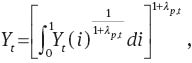
where the elasticity of substitution has a stochastic process:

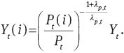
The profit maximization condition of the firm is represented by the demand equation for intermediate good
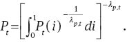
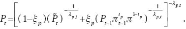
Since the firm makes zero profit in the equilibrium, aggregate price is represented by
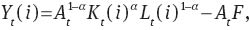
A.2 Intermediate good producer
The firm utilizes the following production technology:
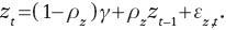
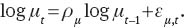
where the growth rate of neutral technology factor At, defined by zt≡ΔlogAt, follows an AR(1) process:
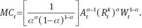
Given the production technology, cost minimization problem results in the following marginal cost function:
The firm chooses the price of its output to maximize its profit as follows:
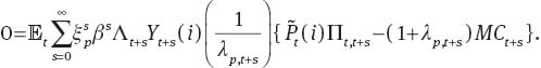
Since
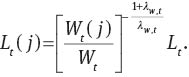
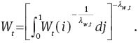
A.3 Employment agencies
Employment agencies combine specialized labor according to the technology
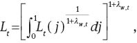
where the elasticity of substitution follows a stochastic process

The firm’s profit maximization condition is represented by the demand for each type of specialized labor
Wage paid by intermediate good producer is
A.4 Household
A.4.1 Model JPT
Preference factor and investment productivity have the following stochastic processes:
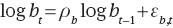
and
Capital service is defined as:
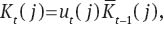
and capital stock is accumulated according to:
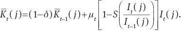
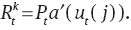
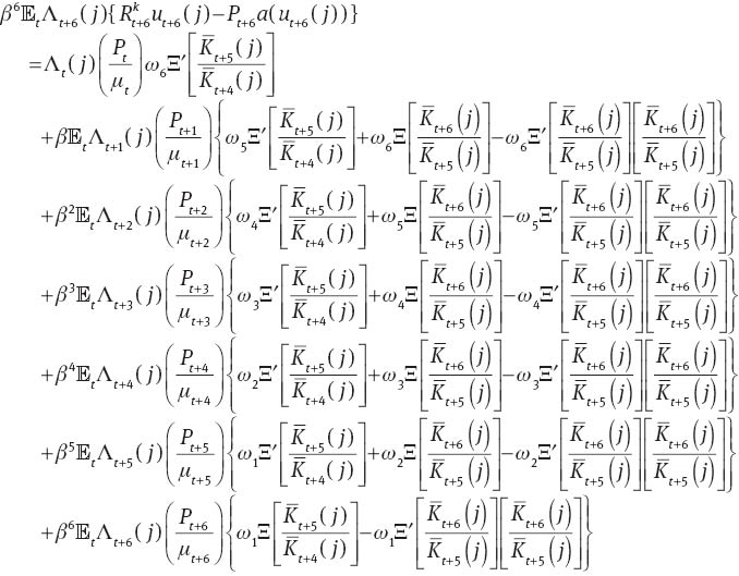
The household’s first order conditions with respect to consumption, government bond, investment, capital stock, and capital utilization are:
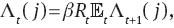
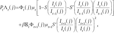

and
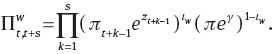
The choice of optimum wage rate is represented by the following equation:
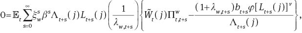
where
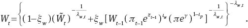
Since the household has only 1–ξw of probability to optimize wage rate in each period, the non-optimizing household would index wage rate according to:
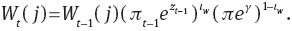
Since
A.4.2 Model Cas
In Model Cas, the law of motion equation (A.17) is replaced by the following equation:

where
A.5 Government
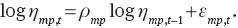
Monetary policy is conducted according to an interest rate rule:
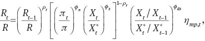
where the monetary policy factor follows a stochastic process:
Government spending is defined as:
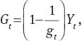
where government spending factor has an AR(1) process:

A.6 Market clearing
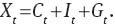
GDP is defined as follows:
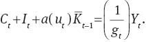
If household budget constraints in equilibrium are summed up over households, then we can derive aggregate resource constraint:
B Description of the data
The data set used for estimation are as follows:
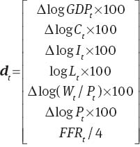
where
The raw data can be described as follows:
| Data | Description | Unit |
|---|---|---|
| RGDP | Real GDP | Bil’s of 2009 USD |
| POP | Civilian noninstitutional population of 16 years or older | Thousands |
| NCND | Nominal personal consumption expenditures on non-durables | Bil’s of 2009 USD |
| NCS | Nominal personal consumption expenditures on services | Bil’s of 2009 USD |
| GDPdef | GDP deflator | 2009=100 |
| NNRPFI | Nominal non-residential private fixed investment | Bil’s of 2009 USD |
| NFBAWH | Nonfarm business, all persons, average weekly hours | 2009=100 |
| CE16index | Index of civilian employment: 16 years or older | 2009=1 |
| POPindex | Index of civilian noninstitutional population of 16 years or older | 2009=1 |
| NFBHC | Nonfarm business, all persons, hourly compensation | 2009=100 |
| FFR | The effective Federal Funds rate | Annual rate, % |
References
Abel, A. B. 1979. Investment and the Value of Capital. Garland, New York.Suche in Google Scholar
Almon, S. 1968. “Lags between Investment Decisions and their Causes.” Review of Economics and Statistics 50: 193–206.10.2307/1926195Suche in Google Scholar
Andrés, J., R. Doménech, and J. Ferri. 2012. “Price Rigidity and the Volatility of Vacancies and Unemployment.” University of Valencia Working Paper.Suche in Google Scholar
Blanchard, O. J., and C. M. Kahn. 1980. “The Solution of Linear Difference Models Under Rational Expectations.” Econometrica 48: 1305–1311.10.2307/1912186Suche in Google Scholar
Boivin, J., and M. P. Giannoni. 2006. “Has Monetary Policy Become more Effective?” The Review of Economics and Statistics 88 (3): 445–462.10.1162/rest.88.3.445Suche in Google Scholar
Bouakez, H., E. Cardia, and F. J. Ruge-Murcia. 2005. “Habit Formation and the Persistence of Monetary Shocks.” Journal of Monetary Economics 52 (6): 1073–1088.10.1016/j.jmoneco.2005.08.009Suche in Google Scholar
Casares, M. 2006. “Time-to-Build, Monetary Shocks, and Aggregate Fluctuations.” Journal of Monetary Economics 53: 1161–1176.10.1016/j.jmoneco.2005.03.014Suche in Google Scholar
Christiano, L. J., M. Eichenbaum, and C. Evans. 2005. “Nominal Rigidities and the Dynamic Effects of a Shock to Monetary Policy.” Journal of Political Economy 113: 1–45.10.1086/426038Suche in Google Scholar
Clarida, R., J. Galí, and M. Gertler. 2000. “Monetary Policy Rules and Macroeconomic Stability: Evidence and Some Theory.” Quarterly Journal of Economics 115 (1): 147–180.10.1162/003355300554692Suche in Google Scholar
Cogley, T., and J. M. Nason. 1995. “Output Dynamics in Real-Business-Cycle Models.” American Economic Review 85: 492–511.Suche in Google Scholar
Dib, A. 2003. “An Estimated Canadian DSGE Model with Nominal and Real Rigidities.” Canadian Journal of Economics 36 (4): 949–972.10.1111/1540-5982.t01-3-00008Suche in Google Scholar
Edge, R. M. 2007. “Time to Build, Time to Plan, Habit Persistence, and the Liquidity Effect.” Journal of Monetary Economics 54: 1644–1669.10.1016/j.jmoneco.2006.07.003Suche in Google Scholar
Favero, C. A., and R. Rovelli. 2003. “Macroeconomic Stability and the Preferences of the Fed: A Formal Analysis, 1961–1998.” Journal of Money, Credit and Banking 35 (4): 545–556.10.1353/mcb.2003.0028Suche in Google Scholar
Galí, J., and L. Gambetti. 2009. “On the Sources of the Great Moderation.” American Economic Journal: Macroeconomics 1 (1): 26–57.10.1257/mac.1.1.26Suche in Google Scholar
Gelman, A., and D. B. Rubin. 1992. “Inference from Iterative Simulation using Multiple Sequences.” Statistical Science 7 (4): 457–511.10.1214/ss/1177011136Suche in Google Scholar
Gertler, M., L. Sala, and A. Trigari. 2008. “An Estimated Monetary DSGE Model with Unemployment and Staggered Nominal Wage Bargaining.” Journal of Money, Credit and Banking 40 (8): 1713–1764.10.1111/j.1538-4616.2008.00180.xSuche in Google Scholar
Gertler, M., and A. Trigari. 2009. “Unemployment Fluctuations with Staggered Nash Wage Bargaining.” Journal of Political Economy 117 (1): 38–86.10.1086/597302Suche in Google Scholar
Geweke, J. 1999. “Using Simulation Methods for Bayesian Econometric Models: Inference, Development, and Communication.” Econometric Review 18 (1): 1–126.10.1080/07474939908800428Suche in Google Scholar
Gomme, P., F. E. Kydland, and P. Rupert. 2001. “Home Production Meets Time to Build.” Journal of Political Economy 109 (5): 1115–1130.10.1086/322829Suche in Google Scholar
Hamilton, J. D. 1994. Time Series Analysis. Princeton: Princeton University Press.Suche in Google Scholar
Hansen, N., S. D. Müller, and P. Koumoutsakos. 2003. “Reducing the Time Complexity of the Derandomized Evolution Strategy with Covariance Matrix Adaptation.” Evolutionary Computation 11 (1): 1–18.10.1162/106365603321828970Suche in Google Scholar
Hayashi, F. 1982. “Tobin’s Marginal Q and Average Q: A Neoclassical Interpretation.” Econometrica 50 (1): 213–224.10.2307/1912538Suche in Google Scholar
Ireland, P. N. 2001. “Sticky-Price Models of the Business Cycle: Specification and Stability.” Journal of Monetary Economics 47: 3–18.10.1016/S0304-3932(00)00047-7Suche in Google Scholar
Johnson, P. A. 1994. “Capital Utilization and Investment When Capital Depreciates in Use: Some Implications and Tests.” Journal of Macroeconomics 16 (2): 243–259.10.1016/0164-0704(94)90069-8Suche in Google Scholar
Jung, Y.-G. 2013a. “An Inference about the Length of the Time-to-Build Period.” Economic Modelling 33: 42–54.10.1016/j.econmod.2013.03.009Suche in Google Scholar
Jung, Y.-G. 2013b. “A New Strategy to Estimate Time-to-Build Completion Rates.” Economics Bulletin 33 (2): 1073–1081.Suche in Google Scholar
Justiniano, A., G. E. Primiceri, and A. Tambalotti. 2010. “Investment Shocks and Business Cycles.” Journal of Monetary Economics 57: 132–145.10.1016/j.jmoneco.2009.12.008Suche in Google Scholar
Kim, J. 2000. “Constructing and Estimating a Realistic Optimizing Model of Monetary Policy.” Journal of Monetary Economics 45: 329–359.10.1016/S0304-3932(99)00054-9Suche in Google Scholar
Klein, P. 2000. “Using the Generalized Schur form to Solve a Multivariate Linear Rational Expectations Model.” Journal of Economic Dynamics and Control 24: 1405–1423.10.1016/S0165-1889(99)00045-7Suche in Google Scholar
Kling, J. L., and T. E. McCue. 1987. “Office Building Investment and the Macroeconomy: Empirical Evidence, 1973–1985.” Journal of the American Real Estate and Urban Economics Association 15: 234–255.10.1111/1540-6229.00430Suche in Google Scholar
Kydland, F. E., and E. C. Prescott. 1982. “Time to Build and Aggregate Fluctuations.” Econometrica 50: 1345–1370.10.2307/1913386Suche in Google Scholar
Mayer, T. 1960. “Plant and Equipment Lead Times.” Journal of Business 33: 127–132.10.1086/294329Suche in Google Scholar
McRae, R. N. 1989. Critical Issues in Electric Power Planning in the 1990s, vol. 1. Calgary: Canadian Energy Research Institute.Suche in Google Scholar
Montgomery, M. R. 1995. “Time-to-build Completion Patterns for Nonresidential Structures: 1961–1991.” Economics Letters 48: 155–163.10.1016/0165-1765(94)00596-TSuche in Google Scholar
Rouwenhorst, K. G. 1991. “Time to Build and Aggregate Fluctuations: A Reconsideration.” Journal of Monetary Economics 27: 241–254.10.1016/0304-3932(91)90043-NSuche in Google Scholar
Sims, C. A. 2002. “Solving Linear Rational Expectations Models.” Computational Economics 20 (1–2): 1–20.10.1023/A:1020517101123Suche in Google Scholar
Smets, F., and R. Wouters. 2007. “Shocks and Frictions in us Business Cycles: A Bayesian DSGE Approach.” American Economic Review 97 (3): 586–606.10.1257/aer.97.3.586Suche in Google Scholar
Wheaton, W. 1987. “The Cyclic Behavior of the National Office Market.” Journal of the American Real Estate and Urban Economics Association 15: 281–299.10.1111/1540-6229.00433Suche in Google Scholar
©2015 by De Gruyter
Artikel in diesem Heft
- Frontmatter
- Advances
- Consumption composition and macroeconomic dynamics
- Evaluating linear approximations in a two-country model with occasionally binding borrowing constraints
- Contributions
- The bank lending channel and monetary policy rules for Eurozone banks: further extensions
- Investment lags and macroeconomic dynamics
- The zero lower bound: frequency, duration, and numerical convergence
- What drives endogenous growth in the United States?
- Environmental policy and economic growth: the macroeconomic implications of the health effect
- US household deleveraging following the Great Recession – a model-based estimate of equilibrium debt
- Price-level instability and international monetary policy coordination
- Households forming macroeconomic expectations: inattentive behavior with social learning
- Topics
- Complementarity and transition to modern economic growth
- Trend inflation and monetary policy rules: determinacy analysis in New Keynesian model with capital accumulation
- Discussions
- Preface to “Reflections on Macroeconometric Modeling” by Ray C. Fair
- Reflections on macroeconometric modeling