Consumption composition and macroeconomic dynamics

A. Solution to the consumer’s optimization problem.

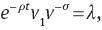
The Hamiltonian function associated with the maximization of (6) subject to (3), (4) and (5) is

H=e−ρtU(c1, c2)+λ(wh+rk−c1−pc2−Ik−phIh)+μ1(Ik−δk)+μ2(Ih−ηh),

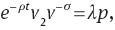
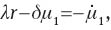
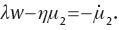
where λ, μ₁, and μ₂ are the co-state variables corresponding to the constraints (3), (4) and (5), respectively. The first order conditions are

(44)e−ρtv1v−σ=λ, (44)

(45)e−ρtv2v−σ=λp, (45)

(46)λ=μ1, (46)

(47)phλ=μ2, (47)

(48)λr−δμ1=−μ˙1, (48)

(49)λw−ημ2=−μ˙2. (49)

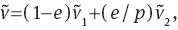
Combining (44) and (45), we obtain Equation (7) and, from log-differentiating this equation with respect to time, we get

(50)[v21v2−v11v1]c˙1+[v22v2−v12v1]c˙2=p˙p. (50)

Since v(c₁, c₂) is linear homogeneous, we establish the following relations:

(51)v=v1c1+v2c2, (51)

(52)v11c1+v12c2=v21c1+v22c2=0. (52)

Using Conditions (51) and (52) in (50), and after some algebra, we obtain

(53)c˙2c2=c˙1c1−ξ(p˙p), (53)

where ξ is the elasticity of substitution of v(·) given in (13). Using (46) and (47), we obtain

phμ1=μ2,

which implies that

p˙hph+μ˙1μ1=μ˙2μ2,

and (8) follows from using (48) and (49). Log-differentiating with respect to time (44), we obtain

−ρ+[v11v1−σ(v1v)]c˙1+[v12v1−σ(v2v)]c˙2=λ˙λ.

By employing the definition of the elasticity of substitution ξ given in (13), we derive

−ρ+[v11v1−σξ(v12v2)]c˙1+(v12v1)(1−σξ)c˙2︸−ε/c2=λ˙λ.

Combining this equation with (46) and (48), and using Conditions (51) and (52), we obtain

−r+δ=−ρ−[v12c1v2][v2c2v1c1+σξ](c˙1c1)−ε(c˙2c2).

Finally, Equations (9) and (10) follow from combining the previous equation with (53) and combining the resulting expression with (51) and (52).

B. Deriving the Euler equation on expenditure

First, we express the solution to the consumer’s problem in terms of total expenditure and the fraction of expenditure on c₂. To this end, we use the linear homogeneity of function v(·) to define

(54)v˜(1−e, e/p)≡v(c1, c2)c, (54)

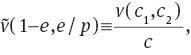
and, moreover, we note that

(55)vi(c1, c2)=v˜i(1−e, e/p), (55)

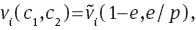
and

(56)vij(c1, c2)=c−1v˜ij(1−e, e/p), (56)

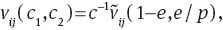
for i={1, 2} and j={1, 2}. Using these properties, we rewrite Condition (7) as

(57)pv˜1=v˜2, (57)

the elasticity of substitution ξ given in (13) as

(58)ξ=v˜2v˜1v˜12v˜, (58)

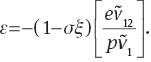
and the Edgeworth elasticity ε given in (14) as

(59)ε=−(1−σξ)[ev˜12pv˜1]. (59)

Since v˜ is also linearly homogeneous, we get

(60)v˜=(1−e)v˜1+(e/p)v˜2, (60)

and

(61)(1−e)v˜11+(e/p)v˜12=(1−e)v˜21+(e/p)v˜22=0. (61)

Condition (60) together with (57) implies that v˜=v˜1. Therefore, the elasticity of substitution ξ can finally be expressed in equilibrium as

(62)ξ=v˜2v˜12. (62)

Using the strict quasiconcavity of v and v˜, we get from applying the implicit function theorem to (57) that

∂e∂p≡E′(p)=v˜1+(e/p2)v˜22−(e/p)v˜12−v˜21+(1/p)v˜22+pv˜11−v˜12.

By using Condition (61), and after some algebra, we obtain

E′(p)=−(ep)(1−e)[pv˜1v˜12−1],

so that (15) follows from using (57) and (62).

Log-differentiating c₁=(1–e)c with respect to time, and combining the resulting expression with (9), we obtain

c˙c=r−ρ−δσ+[εξσ+pE′(p)1−e](p˙p).

By combining the previous equation with (57), (59), (62) and (15), and after some algebra, we obtain (16).

C. Proofs of results

Proof of Proposition 3.1.

1. Consider first the condition α₁=α₂. We can first combine equations (17), (18), (20) and (21) to get z₁=z₂. Therefore, by combining equations (17) and (18), it follows that the relative price between the two consumption goods remains constant and equal to p=A₁/A₂.

2. Let us now consider the condition α₁=α₃. Observe that in this case conditions (17), (19), (20) and (22) imply that z₁=z₃ and, thus, the relative price between the two capitals is constant and given by p_h=A₁/A₃. Equation (8) implies that the ratio w/r remains constant when p_h is constant. Then, from combining (17) and (20) we immediately see that z₁ is constant when p_h is constant. Therefore, both the rental rate r and z₂ are constant as follows from (17) and (19). Finally, equation (18) shows that in this case relative price p between the two consumption goods remains constant.      ■

Proof of Proposition 3.2. The uniqueness of p* follows from the monotonicity of κ(p), which can be shown using (32),

κ′(p)=[(1−α1)A1ψ1α1−1pα2−1α1−α2α3−α1][α1+(α3ψ1φα1−α3α1−α2)p1−α1+α3α1−α2]>(<)0 if α1<(>)α3,

and the fact that limp→0κ(p)=−∞(∞) and limp→∞κ(p)=∞(−∞) when α₁<(>)α₃.

Combining (26), (27) and (28), we obtain

(63)u1=z3−zz3−z1+[E(p)pA2z2α2](z2−z3z3−z1)qz (63)

and

(64)1−u1−u2=z−z1z3−z1+[E(p)pA2z2α2](z1−z2z3−z1)qz. (64)

Given the value of p*, the strict quasiconcavity of v(c₁, c₂) guarantees a unique stationary value of the expenditure shares. Denote by θ˜ the value of 1–E(p*). In a steady state, equations (34) and (33) simplify to

1−u1∗−u2∗=g∗+ηA3(z3∗)α3,

A1u1∗(z1∗)α1z∗−θ˜q∗=g∗+δ.

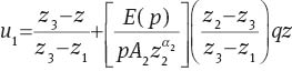
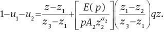
By using (63) and (64), the previous two equations can be rewritten as the following system of two equations:

z∗+(1−θ˜p∗A2(z2∗)α2)︸ϕ1(z1∗−z2∗)q∗z∗=(g∗+ηA3(z3∗)α3)(z3∗−z1∗)+z1∗︸ϕ2,

z3∗+[ϕ1∗(z2∗−z3∗)−(z3∗−z1∗)A1(z1∗)α1]q∗z∗=[(z3∗−z1∗)(g∗+δA1(z1∗)α1)+1]z∗︸φ3.

The steady state values of z* and q* are the unique solution of this system of equations and they are equal to

z∗=ϕ1ϕ2(z2∗−z3∗)+ϕ1(z1∗−z2∗)z3∗−ϕ2(z3∗−z1∗)A1(z1∗)α1ϕ1(z2∗−z3∗)+ϕ1ϕ3(z1∗−z2∗)−z3∗−z1∗A1(z1∗)α1,

and

q∗=ϕ2ϕ3−z3∗[ϕ1ϕ2(z2∗−z3∗)−ϕ2(z3∗−z1∗)A1(z1∗)α1+ϕ1(z1∗−z2∗)z3∗],

where the steady-state values of z_i, i={1, 2, 3}, satisfy zi∗=ψi(p∗)1α1−α3 as follows from (23).      ■

Proof of Proposition 4.1. Let J be the Jacobian matrix evaluated at the steady state of the system of differential equations formed by (32), (37) and (38), ^[13]

J=(∂p˙∂p∂p˙∂z∂p˙∂q∂z˙∂p∂z˙∂z∂z˙∂q∂q˙∂p∂q˙∂z∂q˙∂q),

where

∂p˙∂p=pκ′(p),

∂p˙∂z=0,

∂p˙∂q=0,

∂z˙∂p=z{(A1z1α1z)(∂u1∂p)+(A1u1α1z1α1−1z)(∂z1∂p)︸ϵp−A3z3α3[∂(1−u1−u2)∂p]−A3(1−u1−u2)α3z3α3−1(∂z3∂p)},

∂z˙∂z=z{−A1u1z1α1z2+(A1z1α1z)(∂u1∂z)︸ϵz−A3z3α3[∂(1−u1−u2)∂z]},

∂z˙∂q=z(A1z1α1z)(∂u1∂q)−θ︸ϵq−A3z3α3[∂(1−u1−u2)∂q],

∂q˙∂p=q{[α1(α1−1)A1z1α1−2σ](∂z1∂p)−[(1−σ)(1−θ)σ]κ′(p)−ϵp},

∂q˙∂z=−qϵz,

and

∂q˙∂q=−qϵq.

The determinant of the Jacobian matrix is

Det(J)=(∂p˙∂p)[(∂z˙∂z)(∂q˙∂q)−(∂z˙∂q)(∂q˙∂z)]=zqκ′(p)pA3z3α3M,

where

M=ϵq[∂(1−u1−u2)∂z]−ϵz[∂(1−u1−u2)∂q]={θ(∂u1∂z)−(A1u1z1α1z2)(∂u1∂q)−[(A1z1α1z)(∂u1∂q)−θ](∂u2∂z)+[−A1u1z1α1z2+(A1z1α1z)(∂u1∂z)](∂u2∂q)}.

Using (26), (63) and (64), and after some algebra, M simplifies to

M=−(θz3−z1)[1+ϕ1z2(g∗+δ)+ϕ1z1(A1z1α1−1−g∗−δ)︸N].

Note that N>0 because

A1z1α1−g∗−δ=g∗(σ−α1)+ρ+δ(1−α1)α1>0,

where the inequality follows from the transversality condition, which implies that ρ>(1–σ)g*. Thus, the determinant is given by

Det(J)=−(θzqκ′(p)pA3z3α3z3−z1){1+ϕ1z2(g∗+δ)+ϕ1z1[g∗(σ−α1)+ρ+δ(1−α1)α1]}.

By using (23) and (25), we obtain that z₃>(<)z₁ when α₁<(>)α₃ and, therefore, we derive from the proof of Proposition 3.2 that κ′(p)>(<)0 when z₃>(<)z₁. We then conclude that Det(J)<0. Next, we obtain the value of the trace,

Tr(J)=∂p˙h∂ph+∂z˙∂z+∂q˙∂q={pκ′(p)+A1z1α1(∂u1∂z)−A1u1z1α1z−(A3z3α3z)[∂(1−u1−u2)∂z]−q[(A1z1α1z)(∂u1∂q)−θ]}.

Using (63) and (64), the trace simplifies, after some tedious algebra, to

Tr(J)=α1A1ψ1α1−1pα1−1α1−α2+(1−α1)A1ψ1α1pα3α1−α2φα1−α3α1−α2−(g∗+η)−(g∗+δ).

Making κ(p)=0, we obtain

Tr(J)=2(α1A1ψ1α1−1pα1−1α1−α2−g∗−δ),

and, by using (35) at BGP, we derive

Tr(J)=2[(σ−1)g∗+ρ]>0,

as follows from the transversality condition.

Since the trace of J is positive and the determinant is negative, there exists a unique negative root and the equilibrium is saddle-path stable. When α₁>α₃ the adjustment process of relative price p is stable so that the negative root of the Jacobian J is pκ′(p). Otherwise, the dynamic process of p is unstable In this case, relative price p instantaneously jumps to its stationary value, and the negative root of J is one of the roots obtained from the sub-system of differential equations formed by equations (37) and (38) with p=p* for all t. ^[14]      ■

Proof of Lemma 4.2. Equation (23) shows that all the physical to human capital ratios in the three sectors, z₁, z₂ and z₃, depend positively (negatively) on relative price p when α₁>(<)α₂. We can write the aggregate physical to human capital ratio z=k/h as

(65)z=k1+k2+k3h1+h2+h3, (65)

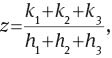
where k_i and h_i are the stocks of physical and human capital used in the production of good i, i={1, 2, 3}. When all the ratios z₁, z₂ and z₃ vary in the same direction, the aggregate physical to human capital ratio z also varies in this direction. For instance, if all the ratios z₁, z₂ and z₃ rise, then the following relationship between the increments of the sectoral capital stocks must apply: Δk₁>Δh₁, Δk₂>Δh₂, and Δk₃>Δh₃. Therefore,

Δk1+Δk2+Δk3>Δh1+Δh2+Δh3.

Using the previous inequality in (65), and the dependence of the ratios z₁, z₂ and z₃ on relative price p, we obtain the monotonically increasing (decreasing) relationship between the aggregate physical to human capital ratio z and relative price p of human capital along the stable manifold when α₁>(<)α₂.

Note that equation (23) implies that lim_p→0z_i=0(∞) when α₁>(<)α₂, with z_i=k_i/h_i, i={1, 2, 3}. This means that either lim_p→0k_i=0(∞) or lim_p→0h_i=∞(0) when α₁>(<)α₂. In both cases, we will get that lim_p→0z=0(∞) if α₁>(<)α₂. However, lim_p→∞z_i=∞(0) when α₁>(<)α₂, with z_i=k_i/h_i, i={1, 2, 3}, which means that either lim_p→∞k_i=∞(0) or limp_→∞h_i=0(∞) when α₁>(<)α₂. In both cases, we will get that lim_p→∞z=∞(0) if α₁>(<)α₂. Therefore, as the ratio z may take potentially any value in the interval (0, ∞), the range of values of the price p along the stable manifold is also (0, ∞).      ■

Proof of Proposition 4.3. In the proof of Proposition 4.1, we have shown that κ′(p)<0 if α₁>α₃. This means that the relative price exhibit a monotonic transition. In addition, Lemma 4.2 states that the stable manifold relating prices and the ratio of capitals is strictly monotone. This implies that the ratio z of capitals must also exhibit a monotonic behavior along the entire transition.      ■

Proof of Proposition 4.4. Given the sign of P′(z) characterized by Lemma 4.2, we conclude from (40) that the growth rate of consumption expenditure γ is increasing (decreasing) when Ω(z)>(<)0. Therefore, the statement of the proposition directly follows from (41). Parts (a) and (d) follow since Ω(z)<0 when χ≤0 and Ω(z)>0 when χ>1σ. For Part (b) note that we get Ω(z)>0 along the transition when z₀>z* and Ω(z)<0 when z0<z¯<z∗. In the first case, the rate of growth of consumption is monotonically decreasing, whereas it exhibits a non-monotonic behavior when z0<z¯. In particular, if z0<z¯ the growth rate of consumption expenditure initially decreases and ends up being increasing with time as the dynamic equilibrium approaches its steady state. In Part (c), we have that Ω(z)>0 along the transition when z₀<z* and Ω(z)<0 when z0>z¯≥z∗. In the first case, the consumption growth rate is monotonically decreasing, whereas it exhibits a non-monotonic behavior when z0>z¯. In particular, if z0>z¯ the growth rate of consumption expenditure initially decreases and becomes eventually increasing as the equilibrium path approaches its steady state.      ■

References

Acemoglu, D., and V. Guerrieri. 2008. “Capital Deepening and Nonbalanced Economic Growth.” Journal of Political Economy 116: 467–498.10.1086/589523Search in Google Scholar
Alvarez-Cuadrado, F. 2008. “Growth Outside the Stable Path: Lessons from the European Reconstruction.” European Economic Review 52: 568–588.10.1016/j.euroecorev.2007.02.003Search in Google Scholar
Alvarez-Cuadrado, F., G. Monterio, and S. Turnovsky. 2004. “Habit Formation, Catching-up with the Joneses, and Economic Growth.” Journal of Economic Growth 9: 47–80.10.1023/B:JOEG.0000023016.26449.ebSearch in Google Scholar
Bond E., P. Wang, and C. Yip. 1996. “A General Two-Sector Model of Endogenous Growth with Human and Physical Capital: Balanced Growth and Transitional Dynamics.” Journal of Economic Theory 68: 149–173.10.1006/jeth.1996.0008Search in Google Scholar
Boppart, T. 2014. “Structural Change and the Kaldor Facts in a Growth Model with Relative Price Effects and Non-Gorman Preferences.” Econometrica, forthcoming.10.3982/ECTA11354Search in Google Scholar
Buera, F. J., and J. P. Kaboski. 2009. “Can Traditional Theories of Structural Change Fit the Data?” Journal of European Economic Association 7: 469–477.10.1162/JEEA.2009.7.2-3.469Search in Google Scholar
Caballé, J., and M. Santos. 1993. “On Endogenous Growth with Physical and Human Capital.” Journal of Political Economy 101: 1042–1067.10.1086/261914Search in Google Scholar
Cooley, T., and E. Prescott. 1995. “Economic Growth and Business Cycles.” In Frontiers of Business Cycle Research, edited by T. Cooley, 1–38. Princeton University Press.10.1515/9780691218052-005Search in Google Scholar
Christiano, L. J. 1989. “Understanding Japan’s Saving Rate: The Reconstruction Hypothesis.” Federal Reserve Bank of Minneapolis Quarterly Review 13: 10–25.10.21034/qr.1322Search in Google Scholar
Echevarria, C. 1997. “Changes in Sectoral Composition Associated with Economic Growth.” International Economic Review 38: 431–452.10.2307/2527382Search in Google Scholar
Fiaschi, D., and A. M. Lavezzi. 2004. “Nonlinear Growth in a Long-run Perspective.” Applied Economic Letters 11: 101–104.10.1080/1350485042000200196Search in Google Scholar
Foellmi, R., and J. Zweimüller. 2008. “Structural Change, Engel’s Consumption Cycles and Kaldor’s Facts of Economic Growth.” Journal of Monetary Economics 55: 1317–1328.10.1016/j.jmoneco.2008.09.001Search in Google Scholar
Hall, R. E. 1988. “Intertemporal Substitution in Consumption.” Journal of Political Economy 96: 339–357.10.1086/261539Search in Google Scholar
Hansen, G., and E. Prescott. 2002. “Malthus to Solow.” American Economic Review 92: 1205–1217.10.1257/00028280260344731Search in Google Scholar
Herrendorf, B., R. Rogerson, and A. Valentinyi. 2013. “Two Perspectives on Preferences and Structural Transformation.” American Economic Review 103: 2752–2789.10.1257/aer.103.7.2752Search in Google Scholar
Jones, L. E., R. E. Manuelli, and P. E. Rosi. 1993. “Optimal taxation in Models of Endogenous Growth.” Journal of Political Economy 101: 485–517.10.1086/261884Search in Google Scholar
Kongsamut, P., S. Rebelo and D. Xie. 2001. “Beyond Balanced Growth.” Review of Economic Studies 68: 869–882.10.1111/1467-937X.00193Search in Google Scholar
Laitner, J. 2000. “Structural Change and Economic Growth.” Review of Economic Studies 67: 545–561.10.1111/1467-937X.00143Search in Google Scholar
Lucas, R. E. 1987. Models of Business Cycles. Basil Blackwell.Search in Google Scholar
Lucas, R. 1988. “On the Mechanics of Economic Development.” Journal of Monetary Economics 22: 3–42.10.1016/0304-3932(88)90168-7Search in Google Scholar
Maddison, A. 2001. The World Economy: A Millennia Perspective. OECD, Paris.10.1787/9789264189980-enSearch in Google Scholar
Mulligan, C., and X. Sala-i-Martín. 1993. “Transitional Dynamics in Two-Sector Models of Endogenous Growth.” Quarterly Journal of Economics 108: 737–773.10.2307/2118407Search in Google Scholar
Ngai, R. 2004. “Barriers and the Transition to Modern Growth.” Journal of Monetary Economics 51: 1353–1383.10.1016/j.jmoneco.2003.12.005Search in Google Scholar
Ngai, R., and C. Pissarides. 2007. “Structural Change in a Multi-sector Model of Growth.” American Economic Review 97: 429–443.10.1257/aer.97.1.429Search in Google Scholar
Papageorgiou, C., and F. Perez-Sebastian. 2006. “Dynamics in a Non-Scale R&D Growth Model: Explaining the Japanese and South Korean Development Experiences.” Journal of Economic Dynamics and Control 30: 901–930.10.1016/j.jedc.2005.03.005Search in Google Scholar
Perez, F., and D. Guillo. 2010. “Reexamining the Role of Land in Economic Growth.” Manuscript.Search in Google Scholar
Perli, R., and P. Sakellaris. 1998. “Human Capital Formation and Business Cycle Persistence.” Journal of Monetary Economics 42: 67–92.10.1016/S0304-3932(98)00011-7Search in Google Scholar
Rebelo, S. 1991. “Long-run Policy Analysis and Long-run Growth.” Journal of Political Economy 99: 500–521.10.1086/261764Search in Google Scholar
Rebelo, S. 1992. “Growth in Open Economies.” Carnegie-Rochester Conference Series on Public Policy 36: 5–46.10.1016/0167-2231(92)90014-ASearch in Google Scholar
Rostow, W. 1960. The Stages of Economic Growth. Oxford: Oxford University Press.Search in Google Scholar
Steger, T. M. 2000. “Economic Growth with Subsistence Consumption.” Journal of Development Economics 62: 343–361.10.1016/S0304-3878(00)00088-2Search in Google Scholar
Steger, T. M. 2006. “Heterogeneous Consumption Goods, Sectoral Change and Economic Growth,” Studies in Nonlinear Dynamics and Econometrics 10 (1): Article 2.10.2202/1558-3708.1309Search in Google Scholar
Uzawa, H. 1965. “Optimum Technical Change in an Aggregative Model of Economic Growth.” International Economic Review 60: 12–31.10.2307/2525621Search in Google Scholar
Valentinyi, A., and B. Herrendorf. 2008. “Measuring factor income shares at the sectoral level.” Review of Economic Dynamics 11: 820–835.10.1016/j.red.2008.02.003Search in Google Scholar
©2015 by De Gruyter
Articles in the same Issue